A Geometric Monte Carlo Algorithm for the Antiferromagnetic Ising model with “Topological” Term at $\theta=\pi$

Abstract

In this work we study the two and three-dimensional antiferromagnetic Ising model with an imaginary magnetic field $i\theta$ at $\theta=\pi$. In order to perform numerical simulations of the system we introduce a new geometric algorithm not affected by the sign problem. Our results for the $2D$ model are in agreement with the analytical solution. We also present new results for the $3D$ model which are qualitatively in agreement with mean-field predictions.

1 Introduction

Since its introduction many years ago, the Ising model has been a prototype statistical system for studying phase transitions and critical phenomena [1]. With the advent of the epoch of computer numerical simulations to study statistical systems, this model has become even more important as a test bench to develop new algorithms. There are many interesting physical systems for which, due to the sign problem, we do not have efficient numerical algorithms. Some examples include QCD at finite density or with a non-vanishing $\theta$ term. This situation has hindered progress in such fields for a long time, and it is thus of great interest to study novel simulation algorithms. In the present work we develop and test a new algorithm, which belongs to a class of “geometric” algorithms [2, 3, 4, 5, 6, 7, 8, 9, 10, 11, 12, 13, 14, 15, 16, 17, 18, 19, 20], and which is applicable to the $D\geq 2$ dimensional antiferromagnetic Ising model with an imaginary magnetic field $i\theta$ (see [21] and [22]) at $\theta=\pi$, with which we are able to solve the sign problem that afflicts this model when using standard algorithms. Preliminary results were presented in [24].

This paper is organized as follows. In Section 2 we introduce the Antiferromagnetic Ising model. In Section 3 we derive our geometric representation of the model. Section 4 is devoted to the construction of the numerical algorithm. In Section 5 we present the numerical results and finally Section 6 contains our conclusions. Some technical details on the ergodicity of the algorithm as well as on the numerical analysis are contained in the appendices.

2 The Antiferromagnetic Ising model with a topological term

We consider the Ising model in $D\geq 2$ dimensions, defined on a hypercubic lattice $\Lambda$ with an even number of sites $L=2n$ in each direction, and with either open or periodic boundary conditions. The Hamiltonian of the model is

$$H[\{s_{x}\},J,B]=-J\sum_{(x,y)\in{\cal B}}s_{x}s_{y}-B\sum_{x}s_{x}\,.$$ (1)

Here the spin variables are $s_{x}=\pm 1$, and the sum $\sum_{(x,y)\in{\cal B}}$ is over the pairs of sites $(x,y)$ that are nearest neighbors; we denote the set of all such pairs by ${\cal B}$. Moreover, $J$ is the coupling between nearest neighbors, and $B$ is an external magnetic field. The reduced Hamiltonian ${\cal H}=H/(k_{B}T)$, where $T$ is the temperature and $k_{B}$ the Boltzmann constant, is written as

$${\cal H}[\{s_{x}\},F,h]=-F\sum_{(x,y)\in{\cal B}}s_{x}s_{y}-\frac{h}{2}\sum_{x}s_{x}\,,$$ (2)

with $F=J/(k_{B}T)$, $h=2B/(k_{B}T)$. As the total number of spins is $L^{D}=(2n)^{D}$, and therefore even, the quantity $Q=\frac{1}{2}\sum_{x}s_{x}$ is an integer number, taking values between $-L^{D}/2$ and $L^{D}/2$. $Q$ can then be thought of as playing the role of a topological charge. It is then worth studying what happens for imaginary values of the reduced magnetic field $h$, i.e., for $h=i\theta$. The topological charge $Q$ is odd under the $Z_{2}$ transformation $s_{x}\to-s_{x}$ $\forall x$: while at $\theta=0$ the system is symmetric under this transformation, for $\theta\neq 0,\pi$ the $Z_{2}$ symmetry of the system is explicitly broken. At $\theta=\pi$ the contribution of the topological charge to the Boltzmann factor amounts to

$$e^{i\pi Q}=(-1)^{Q}=(-1)^{-Q}\,,$$ (3)

i.e., this contribution is $Z_{2}$ invariant, and therefore the $Z_{2}$ symmetry is restored; it has to be checked if it is spontaneously broken or not.

3 Geometric representation of the model

3.1 Partition function

We will now introduce a geometric representation for the model at $h=i\theta=i\pi$. Let us rewrite the partition function of the system,

$$Z(F,\theta=\pi) =\sum_{s_{x}=\pm 1}e^{F\sum_{(x,y)\in{\cal B}}s_{x}s_{y}+i\frac{\pi}{2}\sum_{z}s_{z}}$$ (4)

$$=\sum_{s_{x}=\pm 1}\prod_{(x,y)\in{\cal B}}e^{Fs_{x}s_{y}}\prod_{z}i^{s_{z}}=\sum_{s_{x}=\pm 1}\prod_{(x,y)\in{\cal B}}e^{Fs_{x}s_{y}}\prod_{z}i{s_{z}}$$

$$=i^{V}\sum_{s_{x}=\pm 1}\prod_{(x,y)\in{\cal B}}[\cosh(Fs_{x}s_{y})+\sinh(Fs_{x}s_{y})]\prod_{z}{s_{z}}$$

$$=\sum_{s_{x}=\pm 1}\prod_{(x,y)\in{\cal B}}[\cosh(F)+\sinh(F)s_{x}s_{y}]\prod_{z}{s_{z}}\,,$$

where we have taken into account that the volume of the system, $V=L^{D}$, is a multiple of $4$, and that $\cosh(-x)=\cosh(x)$, $\sinh(-x)=-\sinh(x)$. Note now the following symmetry of this partition function. Define the two staggered lattices $\Lambda^{(1,2)}$ as follows:

$$\Lambda^{(1)} =\{x=(i_{1},\ldots,i_{D})\in\Lambda~{}|~{}(i_{1}+\cdots+i_{D}){\rm mod}\,2=0\}\,,$$ (5)

$$\Lambda^{(2)} =\{x=(i_{1},\ldots,i_{D})\in\Lambda~{}|~{}(i_{1}+\cdots+i_{D}){\rm mod}\,2=1\}\,.$$

Nearest neighbors always belong to different staggered lattices; as a consequence, if we change variables in the sum in Eq. (4) by changing the sign of all the spins in only one of the two staggered lattices, say, $s_{x}\to-s_{x}\,\forall x\in\Lambda^{(2)}$, Eq. (4) becomes

$$Z(F,\theta=\pi) =(-1)^{\frac{L^{D}}{2}}\sum_{s_{x}=\pm 1}\prod_{(x,y)\in{\cal B}}[\cosh(F)-\sinh(F)s_{x}s_{y}]\prod_{z}{s_{z}}$$ (6)

$$=\sum_{s_{x}=\pm 1}\prod_{(x,y)\in{\cal B}}[\cosh(F)-\sinh(F)s_{x}s_{y}]\prod_{z}{s_{z}}\,.$$

Therefore, $Z(F,\theta=\pi)=Z(-F,\theta=\pi)$, i.e., at $\theta=\pi$ the ferromagnetic and antiferromagnetic models are essentially equivalent. In conclusion, we can write

$$Z(F,\theta=\pi)=\sum_{s_{x}=\pm 1}\prod_{(x,y)\in{\cal B}}[\cosh(|F|)+\sinh(|F|)s_{x}s_{y}]\prod_{z}{s_{z}}\,.$$ (7)

Let us denote by ${\cal B}!$ the power set of ${\cal B}$, i.e.,

$${\cal B}!=\{b~{}|~{}b\subseteq{\cal B}\}\,.$$ (8)

A subset $b$ can be seen as a configuration of “active bonds” (we will sometimes also refer to active bonds as “dimers”) between neighboring sites. Let ${\cal N}[b]$ be the number of elements of $b$, i.e., the number of active bonds; clearly, $\bar{\cal N}[b]={\cal N}[{\cal B}]-{\cal N}[b]$ is the number of inactive bonds. Finally, we define the quantity

$$\pi_{x}[(y,z)]=\left\{\begin{aligned} &1&&&&\text{if}~{}x=y~{}\text{or}~{}x=z\,,\\ &0&&&&\text{otherwise}\,,\end{aligned}\right.$$ (9)

and let $\pi_{x}[b]$ be the number of bonds in $b$ that “touch” $x$,

$$\pi_{x}[b]=\sum_{(y,z)\in b}\pi_{x}[(y,z)]\,.$$ (10)

Armed with this notation, we can rewrite the product over pairs of neighboring sites in Eq. (7) as follows,

$$\prod_{(x,y)\in{\cal B}}[\cosh(|F|)+\sinh(|F|)s_{x}s_{y}]=\\ \sum_{b\in{\cal B}!}\cosh(|F|)^{\bar{\cal N}[b]}\sinh(|F|)^{{\cal N}[b]}\prod_{(x,y)\in b}s_{x}s_{y}\,.$$ (11)

The sum over spin configurations in $Z$ vanishes unless each spin appears an even number of times in the product above, and gives a factor of 2 per spin otherwise, that is,

$$\sum_{s_{x}=\pm 1}\prod_{(x,y)\in b}s_{x}s_{y}\prod_{z}s_{z}=\left\{\begin{aligned} &0&&&&\text{if}~{}\exists x\owns\pi_{x}[b]\,{\rm mod}\,2=0\,,\\ &2^{L^{D}}&&&&\text{otherwise}\,.\end{aligned}\right\}$$ (12)

Summarizing,

$$Z(F,\theta=\pi) =2^{L^{D}}\sum_{\begin{subarray}{c}b\in{\cal B}!,\\ \{\pi_{x}[b]{\rm mod}\,2=1\forall x\}\end{subarray}}\cosh(|F|)^{\bar{\cal N}[b]}\sinh(|F|)^{{\cal N}[b]}$$ (13)

$$=2^{L^{D}}\cosh(|F|)^{{\cal N}[{\cal B}]}\sum_{\begin{subarray}{c}b\in{\cal B}!,\\ \{\pi_{x}[b]{\rm mod}\,2=1\forall x\}\end{subarray}}\tanh(|F|)^{{\cal N}[b]}\,.$$

This is the geometric representation that we will use in our algorithm.

3.2 Observables

It is useful to generalize the partition function to the case of variable couplings, i.e,

$${\cal H}\left[\{s_{x}\},\{F_{xy}\},\theta=\pi\right]=-\sum_{(x,y)\in{\cal B}}F_{xy}\,s_{x}s_{y}-i\frac{\pi}{2}\sum_{x}s_{x}\,.$$ (14)

This allows us to calculate all the correlation functions for an even number of spins $\langle s_{x_{1}}s_{x_{2}}\ldots s_{x_{2k}}\rangle$, by taking derivatives with respect to $F_{xy}$ for an appropriate set of $(x,y)$. Indeed, choosing a set of paths ${\cal C}_{1},\ldots{\cal C}_{k}$ connecting the spins pairwise (there are no restrictions on these paths), and then performing derivatives with respect to all the pairs $(x,y)$ appearing in those paths (if a pair appears $m(x,y)$ times, one has to take the $m(x,y)$-th derivative with respect to the corresponding coupling),

$$\langle s_{x_{1}}s_{x_{2}}\ldots s_{x_{2k}}\rangle=Z^{-1}(\{F_{xy}=F\},\theta=\pi)\\ \times\left\{\left[\prod_{(x,y)\in\cup_{j}{\cal C}_{j}}\frac{\partial^{m(x,y)}}{\partial F_{xy}^{m(x,y)}}\right]Z(\{F_{xy}\},\theta=\pi)\right\}\Bigg{|}_{\{F_{xy}\}=\{F\}}\,.$$ (15)

The geometric representation for the partition function with variable couplings is similar to the one obtained for constant coupling, and the final result takes the form

$$Z(\{F_{xy}\},\theta=\pi)=2^{L^{D}}\sum_{\begin{subarray}{c}b\in{\cal B}!,\\ \{\pi_{x}[b]{\rm mod}\,2=1\forall x\}\end{subarray}}\prod_{\begin{subarray}{c}(x,y)\\ (x,y)\notin b\end{subarray}}\cosh(F_{xy})\prod_{\begin{subarray}{c}(x,y)\\ (x,y)\in b\end{subarray}}\sinh(F_{xy})\,.$$ (16)

Taking derivatives with respect to $F_{x_{1}y_{1}},\ldots,F_{x_{l}y_{l}}$, and carrying them inside the summation over $b$, one obtains an extra factor $\coth(F_{x_{i}y_{i}})$ if $(x_{i},y_{i})$ is an active bond of the configuration, i.e., if $(x_{i},y_{i})\in b$, or $\tanh(F_{x_{i},y_{i}})$ if $(x_{i},y_{i})$ is inactive, i.e., $(x_{i},y_{i})\notin b$:

$$\left[\prod_{i=1}^{l}\frac{\partial}{\partial F_{x_{i}y_{i}}}\right]Z(\{F_{xy}\},\theta=\pi)=$$ (17)

$$2^{L^{D}}\sum_{\begin{subarray}{c}b\in{\cal B}!,\\ \{\pi_{x}[b]{\rm mod}\,2=1\forall x\}\end{subarray}}\prod_{i=1}^{l}\left[\tanh(F_{x_{i}y_{i}})(1-\delta_{b}(x_{i},y_{i}))+\coth(F_{x_{i}y_{i}})\delta_{b}(x_{i},y_{i})\right]$$

$$\times\,\,\,\,\,\,\,\,\,\prod_{\begin{subarray}{c}(x,y)\\ (x,y)\notin b\end{subarray}}\cosh(F_{xy})\prod_{\begin{subarray}{c}(x,y)\\ (x,y)\in b\end{subarray}}\sinh(F_{xy})\,,$$

where $\delta_{b}(x,y)=1$ if $(x,y)\in b$, and 0 otherwise. Noting that

$$\tanh(F_{x_{i}y_{i}})(1-\delta_{b}(x_{i},y_{i}))+\coth(F_{x_{i}y_{i}})\delta_{b}(x_{i},y_{i})\\ =\tanh(F_{x_{i}y_{i}})^{1-2\delta_{b}(x_{i},y_{i})}\,,$$ (18)

and setting $F_{xy}=F$, $\forall(x,y)$, we finally obtain

$$\left[\prod_{i=1}^{l}\frac{\partial}{\partial F_{x_{i}y_{i}}}\right]Z(\{F_{xy}\},\theta=\pi)\bigg{|}_{\{F_{xy}\}=\{F\}}=$$ (19)

$$2^{L^{D}}\sum_{\begin{subarray}{c}b\in{\cal B}!,\\ \{\pi_{x}[b]{\rm mod}\,2=1\forall x\}\end{subarray}}\prod_{i=1}^{l}\left[\tanh(F)^{1-2\delta_{b}(x_{i},y_{i})}\right]\prod_{\begin{subarray}{c}(x,y)\\ (x,y)\notin b\end{subarray}}\cosh(F)\prod_{\begin{subarray}{c}(x,y)\\ (x,y)\in b\end{subarray}}\sinh(F)$$

$$=2^{L^{D}}\cosh(F)^{{\cal N}[{\cal B}]}\sum_{\begin{subarray}{c}b\in{\cal B}!,\\ \{\pi_{x}[b]{\rm mod}\,2=1\forall x\}\end{subarray}}\prod_{i=1}^{l}\left[\tanh(F)^{1-2\delta_{b}(x_{i},y_{i})}\right]\tanh(F)^{{\cal N}[b]}\,.$$

Finally, denoting by $\Delta[b;\{x_{i},y_{i}\}]=\sum_{i=1}^{l}\delta_{b}(x_{i},y_{i})$, and dividing by the partition function, we obtain

$$\langle s_{x_{1}}s_{x_{2}}\ldots s_{x_{2k}}\rangle=\frac{\displaystyle\sum_{\begin{subarray}{c}b\in{\cal B}!,\\ \{\pi_{x}[b]{\rm mod}\,2=1\forall x\}\end{subarray}}\tanh(F)^{l-2\Delta[b;\{x_{i},y_{i}\}]}\tanh(F)^{{\cal N}[b]}}{\displaystyle\sum_{\begin{subarray}{c}b\in{\cal B}!,\\ \{\pi_{x}[b]{\rm mod}\,2=1\forall x\}\end{subarray}}\tanh(F)^{{\cal N}[b]}}=$$ (20)

$$\,\,\,\,\,\,\langle\!\langle\tanh(F)^{l-2\Delta[b;\{x_{i},y_{i}\}]}\rangle\!\rangle\,,$$

where the symbol $\langle\!\langle\ldots\rangle\!\rangle$ indicates the average taken with the probability distribution

$$P(b)=\frac{\tanh(F)^{{\cal N}[b]}}{\displaystyle\sum_{\begin{subarray}{c}b\in{\cal B}!,\\ \{\pi_{x}[b]{\rm mod}\,2=1\forall x\}\end{subarray}}\tanh(F)^{{\cal N}[b]}}\,.$$ (21)

As an example, let us write down the two-point correlation function $\langle s_{x}s_{y}\rangle$ for $x$ and $y$ lying on the same lattice axis, e.g., $y=x+l\hat{1}$. Let ${\cal C}$ be a path connecting $x$ and $y$ on the lattice; the simplest choice is a straight-line path ${\cal C}=\cup_{i=1}^{l}(x_{i},y_{i})$ with $y_{i}=x_{i+1}$, $x_{i}=x+(i-1)\hat{1}$ ($i=1,l+1$), $x_{1}=x$ and $y_{l}=y$. We have

$$C(l,F)\equiv\langle s_{x}s_{x+l\hat{1}}\rangle=\langle\!\langle\tanh(F)^{l-2\Delta[b;\{x_{i},y_{i}\}]}\rangle\!\rangle\,,$$ (22)

where $\Delta[b;\{x_{i},y_{i}\}]$ is the number of active bonds in configuration $b$ along the straight-line path connecting $x$ and $x+l\hat{1}$. However, we stress the fact that the specific choice of the path is irrelevant, as they are all equivalent, as long as the endpoints are fixed.

We can also obtain expressions for bulk observables, such as the energy density and the specific heat, by taking derivatives of the partition function with respect to the coupling constant. Using the geometric representation it is easy to see that such observables are directly related to the average number of active bonds and its fluctuations. We denote by $B={\cal N}[b]$ the total number of active bonds, $H_{0}$ is defined as

$$H_{0}=-J\sum_{(x,y)\in{\cal B}}s_{x}s_{y},$$ (23)

and we denote the fluctuations in these quantities by $\Delta H_{0}=H_{0}-\langle H_{0}\rangle$, $\Delta B=B-\langle\!\langle B\rangle\!\rangle$. Then we have the following relations for the energy density $\varepsilon$ and the specific heat $c_{V}$ (we only show for simplicity the relation in the case of periodic boundary conditions):

$$\varepsilon\equiv-\left\langle\frac{H_{0}}{k_{B}TV}\right\rangle=DF\tanh F+\frac{2F}{\sinh 2F}\left\langle\!\!\left\langle\frac{B}{V}\right\rangle\!\!\right\rangle$$ (24)

$$\begin{aligned} c_{V}\equiv\left\langle\frac{1}{V}\left(\frac{\Delta H_{0}}{k_{B}T}\right)^{2}\right\rangle=\frac{DF^{2}}{(\cosh F)^{2}}-\left(\frac{2F}{\sinh 2F}\right)^{2}\cosh 2F\left\langle\!\!\left\langle\frac{B}{V}\right\rangle\!\!\right\rangle+\\ \left(\frac{2F}{\sinh 2F}\right)^{2}\left\langle\!\!\left\langle\frac{1}{V}\left(\Delta B\right)^{2}\right\rangle\!\!\right\rangle\,,\end{aligned}$$ (25)

where $D$ is the dimensionality of the system. For small values of the coupling $F$ the energy density and the specific heat are approximately equal to the average occupation number of the dimers and to its fluctuations:

$$\varepsilon\simeq\left\langle\!\!\left\langle\frac{B}{V}\right\rangle\!\!\right\rangle$$ (26)

$$c_{V}\simeq\left\langle\!\!\left\langle\frac{1}{V}\left(\Delta B\right)^{2}\right\rangle\!\!\right\rangle-\left\langle\!\!\left\langle\frac{B}{V}\right\rangle\!\!\right\rangle$$ (27)

4 Monte Carlo algorithm

In order to perform calculations by means of Monte Carlo methods, we need an efficient algorithm to explore the space of configurations, that as we have seen is given, in the geometric representation, by

$$\tilde{\cal B}\equiv\{b\in{\cal B}!~{}|~{}\pi_{x}[b]\,{\rm mod}\,2=1\,\forall x\}\,,$$ (28)

or, in words, by those configurations for which the number of active bonds touching any site $x$ of the lattice is odd. We will call the set $\tilde{{\cal B}}$ the set of admissible configurations. For simplicity we will describe in detail the algorithm only for $D=2$, as it can be easily generalized to $D>2$.

As far as numerical simulations are concerned, it is enough if we know at least one admissible configuration, and a set of updating rules that take us from one admissible configuration to another and that satisfy detailed balance and ergodicity.

Figure 1: Site $x^{*}$ on the dual lattice in $2D$. The dashed lines indicate bonds whose state is not specified.

To describe the updating rules we found convenient to work with the dual lattice (equivalently, the set of squares of the original lattice). Let us denote a point in the dual lattice by $x^{*}$ , and let us enumerate the four links of the corresponding square in anticlockwise order, as shown in Fig. (1). To describe a configuration of bonds, we introduce for each site of the dual lattice a vector with four components, $A(x^{*})\equiv(A_{1}(x^{*}),A_{2}(x^{*}),A_{3}(x^{*}),A_{4}(x^{*}))$, defined such that $A_{i}(x^{*})=1$ if the corresponding bond is active and $A_{i}(x^{*})=0$ if it is inactive. The bond configuration is completely specified by the dual lattice field $A(x^{*})$, although this description is redundant: indeed, one has that $A_{3}(x^{*})=A_{1}(x^{*}+\hat{1})$ and $A_{2}(x^{*})=A_{4}(x^{*}+\hat{2})$. In Table 1 we show all the possible configurations of a given square on the lattice, i.e., a point $x^{*}$ in the dual lattice. The graphs $S(x^{*})$ corresponding to these configurations, and the number of active bonds, $w(x^{*})=\sum_{i=1}^{4}A_{i}(x^{*})$, are also shown.

$S(x^{*})$	$w(x^{*})$	$A(x^{*})$	$S(x^{*})$	$w(x^{*})$	$A(x^{*})$
	0	$(0,0,0,0)$		2	$(0,1,1,0)$
	1	$(1,0,0,0)$		2	$(0,1,0,1)$
	1	$(0,1,0,0)$		2	$(0,0,1,1)$
	1	$(0,0,1,0)$		3	$(1,1,1,0)$
	1	$(0,0,0,1)$		3	$(1,1,0,1)$
	2	$(1,1,0,0)$		3	$(1,0,1,1)$
	2	$(1,0,1,0)$		3	$(0,1,1,1)$
	2	$(1,0,0,1)$		4	$(1,1,1,1)$

Table 1: Possible configurations at a dual lattice site $x^{*}$. Active bonds are indicated by a solid line, inactive bonds by no line. The quantity $w(x^{*})=\sum_{i=1}^{4}A_{i}(x^{*})$ is the number of active bonds surrounding $x^{*}$.

Suppose now that we are given an admissible configuration, and we want to update it to a new admissible configuration. This requires updating some bonds by changing their state, i.e., $A_{i}(x^{*})\to 1-A_{i}(x^{*})$. A general set of updated bonds defines a (possibly disconnected) path on the direct lattice. If this path has an open end, by definition this means that the end site is touched by a single updated bond. As a consequence, the parity of the number of active bonds touching this site would change from odd to even under the update, and the resulting configuration would not be admissible. The most general admissible update consists therefore in changing the state of bonds belonging to a closed (possibly disconnected) path. This is easily seen to be equivalent to perform consecutive updates on the set of elementary squares that cover that part of the lattice enclosed by the path, each elementary update consisting in changing the state of all the bonds surrounding each one of the elementary squares. In higher dimensions, this set is replaced by the elementary squares on a lattice surface having the path as boundary; any such surface yields the same net update of bonds.

In terms of $A(x^{*})$, an elementary update consists in the following replacement,

$$A(x^{*})\to{\cal C}A(x^{*})\equiv I-A(x^{*})\,,$$ (29)

where ${\cal C}$ stands for conjugation, and where we have introduced the vector $I=(1,1,1,1)$. Under conjugation, $A_{i}(x^{*})\to 1-A_{i}(x^{*})$, $i=1,\ldots 4$; clearly, ${\cal C}^{2}={\cal I}$, where ${\cal I}$ is the identity, ${\cal I}A(x^{*})=A(x^{*})$. The variation $\Delta w(x^{*})$ in the number of active bonds under conjugation is given by

$$\Delta w(x^{*})=\sum_{i=1}^{4}{\cal C}A_{i}(x^{*})-A_{i}(x^{*})=\sum_{i=1}^{4}I_{i}-2A_{i}(x^{*})=2[2-w(x^{*})]\,.$$ (30)

$S(x^{*})$	$A(x^{*})$	$\hat{\cal C}S(x^{*})$	${\cal C}A(x^{*})$	$\Delta w(x^{*})$
	$(0,0,0,0)$		$(1,1,1,1)$	4
	$(1,0,0,0)$		$(0,1,1,1)$	2
	$(0,1,0,0)$		$(1,0,1,1)$	2
	$(0,0,1,0)$		$(1,1,0,1)$	2
	$(0,0,0,1)$		$(1,1,1,0)$	2
	$(1,1,0,0)$		$(0,0,1,1)$	0
	$(1,0,1,0)$		$(0,1,0,1)$	0
	$(1,0,0,1)$		$(0,1,1,0)$	0

Table 2: Transformation of configurations under conjugation ${\cal C}$. Acted upon a graph, we denote the transformation with a hat. The quantity $\Delta w(x^{*})$ is the variation in the number of active bonds when passing from $S(x^{*})$ to $\hat{\cal C}S(x^{*})$. As $\hat{\cal C}$ is an involution, $\hat{\cal C}[\hat{\cal C}S(x^{*})]=S(x^{*})$, so the conjugate of a configuration in column 3 is the corresponding configuration in column 1, and the variation of the number of active bonds changes sign when passing from a configuration in column 3 to the corresponding configuration in column 1.

In Table 2 we show the pairs of configurations of an elementary square connected by conjugation, together with $\Delta w(x^{*})$. These updating steps can be applied independently to all the sites of the dual lattice, and are clearly reversible. We have now the ingredients to set up the first version of a Metropolis algorithm (Algorithm 1).

Algorithm 1

1. At a given site $x^{*}$ of the dual lattice, compute $\Delta w(x^{*})$ corresponding to a conjugation step.

2. If $\Delta w(x^{*})\leq 0$, accept the step.

3. If $\Delta w(x^{*})>0$, take a random number $r\in[0,1]$. If $r\leq\tanh(|F|)^{\Delta w(x^{*})}$, accept the step, otherwise reject it (note that in this case $\tanh(|F|)^{\Delta w(x^{*})}\leq 1$).

4. Repeat the procedure for all the dual lattice sites.

It is easy to see that this algorithm satisfies detailed balance. The only question remaining is that of the ergodicity of the algorithm.

4.1 Ergodicity

Concerning ergodicity the situation is slightly different for open or periodic boundary conditions.

The simplest case is that of open boundaries. In this case we can prove (A.1) that all the admissible configurations can be transformed to the same configuration through a sequence of conjugation moves. As these transformations are reversible, any admissible configuration is connected to all the others. Therefore in this case algorithm 1 is ergodic and can be used as is to simulate the system.

The case of periodic boundary conditions is slightly more complicated. One can see that in this case, the total number of vertical (respectively horizontal) active bonds modulo 2 on any given row (respectively, column) of the dual lattice is conserved under the updating moves, and moreover is the same for any row (column). Calling these numbers vertical and horizontal parity, $P_{V}$ and $P_{H}$, respectively, this defines four different “sectors” of admissible configurations, classified by parities ($P_{V},P_{H}$) $\in$ $\{(0,0),(1,0),(0,1),(1,1)\}$. It can be shown that the updating moves are ergodic within each sector separately (A.2). Therefore we have to modify slightly algorithm 1 to obtain an ergodic algorithm (algorithm 2).

Algorithm 2

1. Start from a configuration of parity, say, $(0,0)$.

2. After a certain number of sweeps through the whole lattice, using algorithm 1, propose a change of the parity $P_{H}$ of the configuration, by proposing the inversion of the state of all the horizontal bonds on a row $i=i_{0}$, $j=1,\ldots L$, of the direct lattice, chosen randomly, so (possibly) passing to a configuration of parity $(0,1)$ with probability $\tanh(|F|)^{\Delta\tilde{w}}$, where

   $$\Delta\tilde{w}=\sum_{j=1}^{L}\left({\cal C}B_{H}(i_{0},j)-B_{H}(i_{0},j)\right)=L-2\sum_{j=1}^{L}B_{H}(i_{0},j)\,,$$ (31)

   and we have denoted $B_{H}(i,j)=A_{1}(i,j)$, and ${\cal C}B_{H}(i,j)=1-B_{H}(i,j)$.

3. After the same number of sweeps through the whole lattice, (try to) change the parity $P_{V}$ of the configuration by proposing the inversion of the state of all the vertical bonds on a column $j=j_{0}$, $i=1,\ldots L$, of the direct lattice, chosen randomly, so (possibly) passing to a configuration of parity $(1,1)$, if the proposal in the previous point has been accepted, or $(1,0)$, if the proposal in the previous point has been rejected, with probability $\tanh(|F|)^{\Delta\tilde{w}}$, where now

   $$\Delta\tilde{w}=\sum_{i=1}^{L}\left({\cal C}B_{V}(i,j_{0})-B_{V}(i,j_{0})\right)=L-2\sum_{i=1}^{L}B_{V}(i,j_{0})\,,$$ (32)

   and we have denoted $B_{V}(i,j)=A_{4}(i,j)$, and ${\cal C}B_{V}(i,j)=1-B_{V}(i,j)$.

4. Iterate the procedure.

The case of higher dimensionality is a straightforward generalization of the algorithms presented here, obtained by applying algorithm 1 to all the elementary squares of the lattice, and by taking into account that for periodic boundary conditions there are now $2^{D}$ “sectors”, classified by the $D$ parities defined in analogy to the $2D$ case.

5 Numerical results

We have performed numerical simulations of both the $2D$ and the $3D$ models using the algorithms discussed previously.

First of all, we tested the algorithms in the case of periodic boundary conditions. The acceptance rate of the global update varies widely with both the coupling and the size of the system. For example, for the $2D$ model at $F=-1.0$ the acceptance rate drops from about $60\%$ at $L=16$ to about $30\%$ at $L=64$; for a smaller coupling, $F=-0.6$, the acceptance rate drops from $27\%$ at $L=16$ to $3\%$ at $L=64$.

Then we checked that the bounds on the number of active bonds in each configuration of our system ( B) and also on the average of this quantity ( C) were respected. For simplicity we only show in Figs. (2) the average number of active bonds.

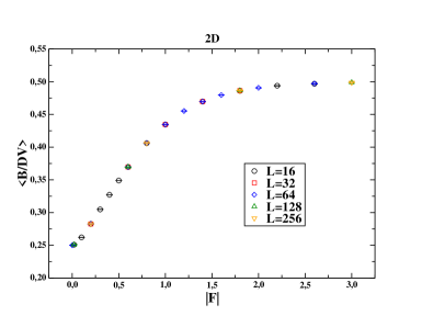
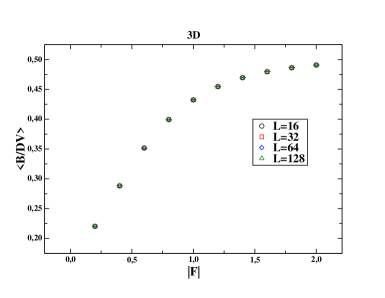
Figure 2: Average number of active bonds normalized by the total number of bonds as a function of $|F|$ for different lattice sizes $L$ for the $2D$ model (top) and $3D$ model (bottom).

Then we calculated the correlation functions (22) as well as the energy density (24) and the specific heat (25) both for the two-dimensional and three-dimensional systems. We have evaluated these quantities for different values of the coupling $F$ and various volumes, with lattice sizes ranging from $L=16$ to $L=1024$. Simulations were done collecting $100$k measurements for each value of $F$. We discarded between $10$k and $20$k configurations at the beginning of each run in order to ensure thermalization. The data analysis was done using the jackknife method over bins at different blocking levels.

In Figs. (3), (4) and (5) we show how the correlation functions depend on the distance $d$, both for the $2D$ and $3D$ models, choosing different antiferromagnetic couplings $F<0$ and varying the lattice volume $V$. In Fig. (6) we show the staggered and the standard magnetization squared in the $2D$ model for two values of the coupling $F$, together with a solid line indicating the analytical result. As can be seen the staggered magnetization squared is always different from zero while the standard magnetization vanishes for all values of the coupling $F$, and the results are in perfect agreement with the analytical solution of Refs. [21, 22, 23]. In Fig. (7) we show the corresponding results for the $3D$ model at the same values of the coupling, as well as the mean-field prediction for the staggered magnetization obtained in Ref. [25]. Again the standard magnetization vanishes, whereas the staggered one does not, and its value is close to the mean-field prediction for large values of the coupling $|F|$. Therefore, despite the vanishing of the standard magnetization, the $Z_{2}$ symmetry of the system is spontaneously broken both in the $2D$ and in the $3D$ models. We can also notice an apparent decrease of $C(d,F)$ at large $d$ for small values of the coupling $F$ both for the $2D$ and $3D$ models. This is due to the heavy-tailed distributions of the correlators, which are also responsible for the noisy behavior seen at large $d$. In Fig. (8) we show the probability distributions of the logarithm of the correlators for a lattice size $L=64$ and for $F=-0.4$ and $F=-2.0$. Clearly we notice that for a small coupling $|F|$ the values are spread in a wider range than for $F=-2.0$; also a long tail develops for large distances $d$, thus making more difficult a precise evaluation of the correlators. Finally, in Figs. (9) and (10) we show the energy density $\varepsilon$ and the specific heat $c_{V}$ as a function of $|F|$ for various lattice sizes $L$. The solid lines present in the figures for the $2D$ model are the analytical results for these quantities [22]. We can see that the energy density and the specific heat do not show any sign of singular behavior in $F$ for the range of couplings studied.

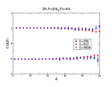
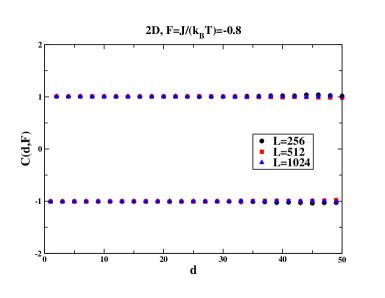
Figure 3: Dependence of the correlation functions on the distance $d$ for different values of the coupling $F$ and for various lattice sizes $L$ in the $2D$ model.

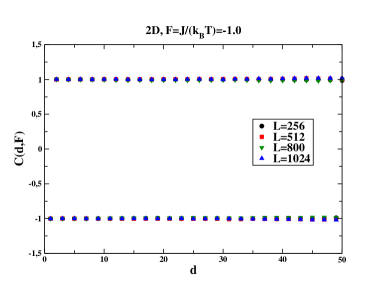
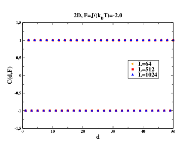
Figure 4: Dependence of the correlation functions on the distance $d$ for different values of the coupling $F$ and for various lattice sizes $L$ in the $2D$ model (continued).

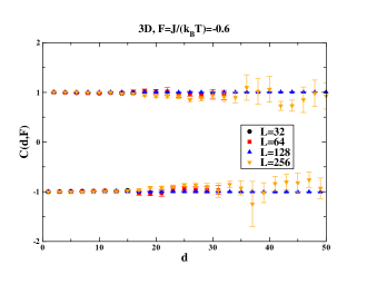
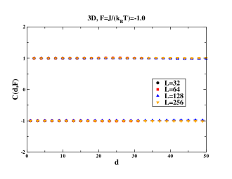
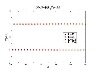
Figure 5: Dependence of the correlation functions on the distance $d$ for different values of the coupling $F$ and for various lattice sizes $L$ in the $3D$ model.

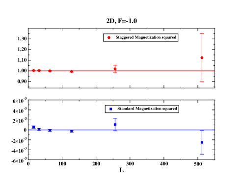
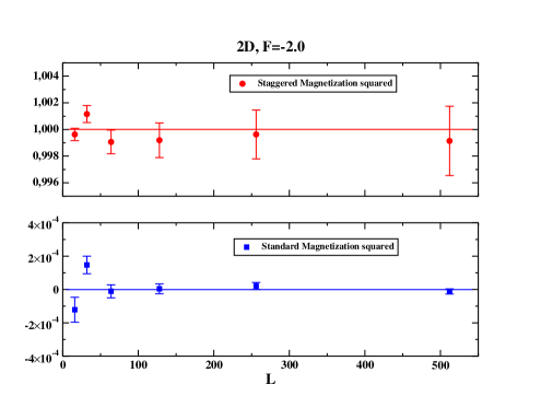
Figure 6: Standard and staggered magnetization squared for two values of the coupling $F$ for the $2D$ model. The red line indicates the analytical prediction (Eq. (53), D), whereas the blue line is the zero value.

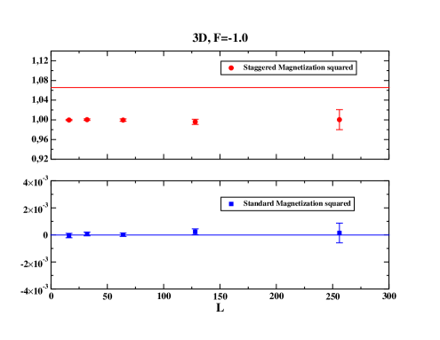
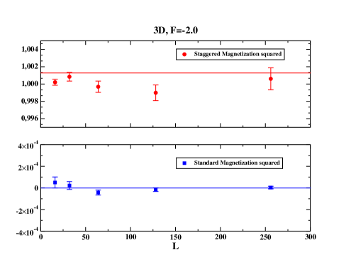
Figure 7: Standard and staggered magnetization squared for two values of the coupling $F$ for the $3D$ model. The red line indicates the mean-field prediction [25], whereas the blue line is the zero value.

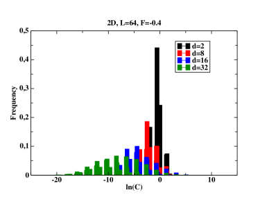
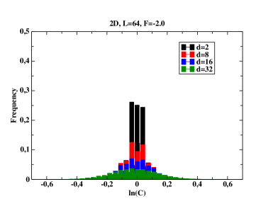
Figure 8: Behavior of the probability distributions of the logarithm of the correlators in the $2D$ model for two different values of the coupling $F$.

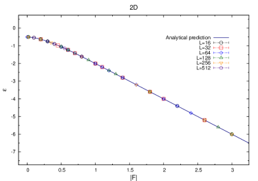
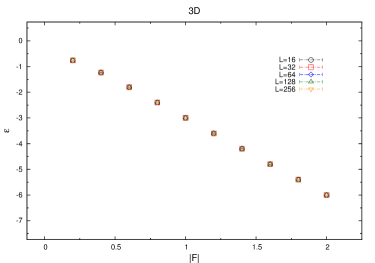
Figure 9: Energy density $\varepsilon$ as a function of $|F|$ for various lattice sizes $L$ for the $2D$ model (top) and $3D$ model (bottom). The analytical result for the $2D$ model is also plotted for comparison.

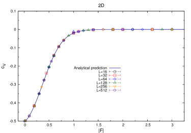
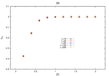
Figure 10: Specific heat $c_{V}$ as a function of $|F|$ for various lattice sizes $L$ for the $2D$ model (top) and the $3D$ model (bottom). The analytical result for the $2D$ model is also plotted for comparison.

6 Conclusions

In this paper we studied the $2D$ and $3D$ antiferromagnetic Ising model with a “topological” $\theta$-term at $\theta=\pi$. For this model we introduced a new geometric algorithm free from the sign problem.

The numerical part of the work has been devoted to testing the algorithm for the two-dimensional model against known analytical results, with which we obtain perfect agreement, and then afterwards to study the three-dimensional system. Our findings strongly support the scenario that, despite the vanishing of the standard magnetization, the staggered magnetization is non-zero for all $D\geq 2$, and therefore the $Z_{2}$ symmetry is spontaneously broken for all values of $F$ at $\theta=\pi$.

It would be interesting to study whether it is possible to introduce a “worm” in our algorithm, in the spirit of [2]. This could change the dynamics of the system; in particular an implementation that allows the worm to wind through the lattice might be able to tunnel between the different parity sectors. We leave the study of such a possibility for a future work.

7 Acknowledgments

The work was funded by MICINN (under grant FPA2012-35453 and FPA2009-09638), DGIID-DGA (grant 2007-E24/2), and by the EU under ITN-STRONGnet (PITN-GA-2009-238353). EF was supported by the MICINN Ramon y Cajal program. MG is supported by the Hungarian Academy of Sciences under “Lendület” grant No. LP2011-011, and partially by MICINN under the CPAN project CSD2007-00042 from the Consolider-Ingenio2010 program.

Appendix A Ergodicity

A.1 Open boundary conditions for the $2D$ model

Consider a $2D$ $N\times N$ square lattice with open boundary conditions. In this case algorithm 1 is ergodic. The basic idea of the proof is to perform transformations that “shift” all the vertical active bonds to the left. This can be accomplished by performing transformations according to the rules listed in Table 3, starting from the upper-right corner of the dual lattice, proceeding downward along a column of the dual lattice, and then moving to the column to the left. We call this transformation “reduction”, which we denote with ${\cal R}$. It is easily seen from Table 3 that it coincides with the identity if $A_{2}(x^{*})=0$, and with conjugation if $A_{2}(x^{*})=1$, i.e.,

$${\cal R}A(x^{*})=\delta_{A_{2},0}\,{\cal I}A(x^{*})+\delta_{A_{2},1}\,{\cal C}A(x^{*}).$$ (33)

In the case of open boundary conditions, the sites of the dual lattice are $x^{*}(i,j)$ with $i,j\in\{1,\ldots,N-1\}$. By construction, after ${\cal R}$ has been applied to the right-most column of the dual lattice, the resulting configuration will not have any vertical bond on the right-hand side of this column, i.e., $A_{2}(x^{*})=0$ for $x^{*}(i,N-1)$, $i\in\{1,\ldots,N-1\}$, and only horizontal bonds will be present. As ${\cal R}$ transforms an admissible configuration into another admissible configuration, the only possibility is that all the horizontal bonds of the right-most column of the dual lattice are active, as the rightmost sites of the direct lattice need to be touched by at least one active bond and they cannot have more than one (see Fig. (11)). We now apply ${\cal R}$ to the following column: as the vertical bonds move to the left, and all the sites in the before-last column of the direct lattice already have an active bond, the horizontal bonds in the before-last column of the dual lattice must be inactive (see Fig. (12)). If we now repeat the procedure, we find ourselves as after the first step: there is a column of sites of the direct lattice with no vertical bonds, and no horizontal bonds to the right, exactly as the right boundary of the lattice. Therefore, the result iterates for pairs of columns of the dual lattice, until we reach the left boundary. As all the sites are already connected horizontally to the right, and as the uppermost site can have at most a single vertical bond, it is easy to see that no vertical bond can appear. We have then reduced the initial configuration to the reduced configuration of Fig. (13). As no reference has been made to the specific form of the initial configuration, the procedure applies equally to any admissible configuration, which completes the proof of ergodicity for open boundary conditions. This also provides an admissible configuration, so completing the construction.

$S(x^{*})$	$A(x^{*})$	$\hat{\cal R}S(x^{*})$	${\cal R}A(x^{*})$
	$(0,0,0,0)$		$(0,0,0,0)$
	$(1,0,0,0)$		$(1,0,0,0)$
	$(0,1,0,0)$		$(1,0,1,1)$
	$(0,0,1,0)$		$(0,0,1,0)$
	$(0,0,0,1)$		$(0,0,0,1)$
	$(1,1,0,0)$		$(0,0,1,1)$
	$(1,0,1,0)$		$(1,0,1,0)$
	$(1,0,0,1)$		$(1,0,0,1)$
	$(0,1,1,0)$		$(1,0,0,1)$
	$(0,1,0,1)$		$(0,1,0,1)$
	$(0,0,1,1)$		$(0,0,1,1)$
	$(1,1,1,0)$		$(0,0,0,1)$
	$(1,1,0,1)$		$(0,0,1,0)$
	$(1,0,1,1)$		$(1,0,1,1)$
	$(0,1,1,1)$		$(1,0,0,0)$
	$(1,1,1,1)$		$(0,0,0,0)$

Table 3: Reduction: it coincides with the identity if $A_{2}=0$, and with conjugation if $A_{2}=1$, i.e., ${\cal R}=\delta_{A_{2},0}\,{\cal I}+\delta_{A_{2},1}\,{\cal C}$.

Figure 11: Right-most column of the dual lattice (using open boundary conditions) after the first step of reduction. The state of the vertical bonds inside the rectangle is not specified.

Figure 12: The two right-most columns of the dual lattice (using open boundary conditions) after the second step of reduction.

Figure 13: Reduced configuration, after completing the reduction process.

A.2 Periodic boundary conditions for the $2D$ model

Consider a $2D$ $N\times N$ square lattice with periodic boundary conditions. In this case, the sites of the dual lattice are $x^{*}(i,j)$ with $i,j\in\{1,\ldots,N\}$, and are closed as well by periodic boundary conditions. We start by applying ${\cal R}$ to column $N$ of the dual lattice. Again, after this procedure there are no vertical bonds active on the right-hand side of the column; however, this time the right-most sites of the direct lattice can have horizontal active bonds entering from the left or from the right, due to the periodic boundary conditions (see Fig. (14)). There are $2^{N}$ possibilities, according to the position of the horizontal bonds (left or right). Repeating the procedure for column $N-1$, one immediately sees that the active horizontal links must be the same as in column 1, as there are no other possibilities due to the absence of vertical bonds in column $N-1$ of the direct lattice (see Fig. (15)). Repeating again, we find for column $N-2$ the same configuration of horizontal bonds of column $N$, and so on. Since there is now an even number of columns on the dual lattice, the final pattern will be $N/2$ identical pairs of columns on the dual lattice, with all the odd columns equal to each other, and all the even columns equal to each other.

At first sight, one could think that there are therefore $2^{N}$ reduced configurations instead of one (see Fig. (16)). At second sight, one could think that there are even more, as it is possible that all the vertical bonds in column 1 of the direct lattice are active (see Fig. (17)): in this case all the sites in this column have two more active bonds (vertical bonds are however absent in the rest of the lattice, by construction). However, one can show that many of these configurations, that we call almost-reduced, can be transformed into one another: by direct inspection, one can show that a configuration with two horizontal bonds on the right of two adjacent sites can be transformed into the configuration with two bonds on the left of the same two adjacent sites, all the rest unchanged (and vice-versa); and that a configuration with one bond on the right and one on the left of two adjacent sites can be transformed into the configuration with the first bond on the left and the second one on the right of the same two adjacent sites, all the rest unchanged. In the case without vertical bonds, it suffices to apply a conjugation to a site of the dual lattice belonging to the row corresponding to the two given sites, and then repeat the reduction procedure; in the case with vertical bonds, it is enough to repeat the reduction procedure along the whole lattice (see Fig. (18)).

Exploiting these equivalences, one can “swap” pairs of bonds, finally reducing to one of the four configurations of Fig. (19). However, it is not possible to transform one of these configurations into one another by means of our admissible moves. To see this, define the number of active vertical bonds on row $i$ of the dual lattice,

$$N_{V}(i)=\sum_{j=1}^{N}A_{4}(i,j)=\frac{1}{2}\sum_{j=1}^{N}A_{4}(i,j)+A_{2}(i,j)\,,\quad N_{V}(i)\in\mathbb{N}\,,$$ (34)

and the number of active horizontal bonds on column $j$ of the dual lattice,

$$N_{H}(j)=\sum_{i=1}^{N}A_{1}(i,j)=\frac{1}{2}\sum_{i=1}^{N}A_{1}(i,j)+A_{3}(i,j)\,,\quad N_{H}(j)\in\mathbb{N}\,.$$ (35)

Observing that the admissible updates always change $A_{1}(i,j)+A_{3}(i,j)$ and $A_{4}(i,j)+A_{2}(i,j)$ by $0$ or $\pm 2$, one has that the vertical parity $P_{V}(i)=N_{V}(i)\,{\rm mod}\,2$ and the horizontal parity $P_{H}(j)=N_{H}(j)\,{\rm mod}\,2$ are conserved under admissible moves. It is evident that for each of the four configurations of Fig. (19), $P_{V}(i)=P_{V}\,\forall i$ and of $P_{H}(j)=P_{H}\,\forall j$, due to the horizontal periodicity of the configuration, and moreover that these configurations have different values of ($P_{V},P_{H}$). As these quantities are conserved, we have that $P_{V}(i)=P_{V}\,\forall i$ and $P_{H}(j)=P_{H}\,\forall j$ also for a generic configuration, which under ${\cal R}$ will be transformed to the reduced configuration with the same pair $(P_{V},P_{H})$.

Figure 14: The $N$th and first columns of the dual lattice (using periodic boundary conditions) after the first step of reduction. (Numbers in the figure refer to columns of the direct lattice).

Figure 15: The $N-1$th, $N$th and first columns of the dual lattice (using periodic boundary conditions) after the first step of reduction.

Figure 16: A possible almost-reduced configuration. The same pattern is repeated along the whole lattice.

Figure 17: Another possible almost-reduced configuration, with all the vertical bonds of column 1 in active state, winding around the lattice. Only the pattern of horizontal bonds is repeated along the whole lattice.

Figure 18: Allowed transformations of a pair of adjacent rows in the almost-reduced configurations. Only the basic block is drawn.

Figure 19: The four inequivalent reduced configurations for periodic boundary conditions. The pair $(P_{V},P_{H})$ is reported above each configuration.

A.3 Ergodicity in the $3D$ model

Consider a $3D$ cubic $N\times N\times N$ lattice, with $N$ even, and a configuration of bonds satisfying the constraint that every site is touched by an odd number of bonds. We define plaquette update (PU) the process of inverting the state (active/inactive) of all the bonds surrounding an elementary square of the lattice. We denote by $P_{\mu\nu}(n)$ the square formed by the links $(n,n+\hat{\mu})$, $(n+\hat{\mu},n+\hat{\mu}+\hat{\nu})$, $(n+\hat{\mu}+\hat{\nu},n+\hat{\nu})$ and $(n+\hat{\nu},n)$, with $\mu,\nu=1,2,3$ and $n=(n_{1},n_{2},n_{3})$ where $n_{i}=1,2,\ldots,N$.

We now show that by means of PU’s it is possible to transform any admissible configuration into any other in the case of open boundary conditions (obc), while in the case of periodic boundary conditions (pbc) it is necessary to supplement these transformations with a few global transformations. In this way we can construct an ergodic algorithm. The strategy is to reduce any admissible configuration to one and the same, “elementary” configuration.

The proof is as follows. Consider the squares lying in the $(1,2)$ planes of the lattice. Fix $n_{1}=N-1$, and $\forall~{}n_{2},n_{3}$ apply a PU on the plaquette $P_{12}(n)$ if the rightmost bond (i.e., the one on the link $(n+\hat{1},n+\hat{1}+\hat{2})$) is active, otherwise leave it untouched. For obc $n_{2}=1,2,\ldots,N-1$ and $n_{3}=1,2,\ldots,N$, while for pbc $n_{2}=1,2,\ldots,N$ and $n_{3}=1,2,\ldots,N$. After this sequence of transformations, all the bonds on the links $(n+\hat{1},n+\hat{1}+\hat{2})$ at $n_{1}=N-1$ are made inactive. Repeat now this procedure for $n_{1}=N-2,N-3,\ldots,1$. As a result, all the bonds on the links $(n+\hat{1},n+\hat{1}+\hat{2})$ (i.e. along direction $2$) for $n_{1}=1,\ldots,N-1$, $n_{2}=1,\ldots,N-1$ (obc) or $n_{2}=1,\ldots,N$ (pbc) and $n_{3}=1,\ldots,N$ are made inactive.

Consider now the squares lying in the $(3,1)$ plane, and starting from $n_{1}=N-1$, apply a PU on the plaquette $P_{31}(n)$ if the rightmost bond (i.e., the one on the link $(n+\hat{1},n+\hat{1}+\hat{3})$) is active, otherwise leave it untouched. For obc $n_{3}=1,2,\ldots,N-1$ and $n_{2}=1,2,\ldots,N$, while for pbc $n_{3}=1,2,\ldots,N$ and $n_{2}=1,2,\ldots,N$; repeat then the procedure for $n_{1}=N-2,N-3,\ldots,1$, so that in the end all the bonds on the links $(n+\hat{1},n+\hat{1}+\hat{3})$ (i.e. along direction $3$) for $n_{1}=1,\ldots,N-1$, $n_{3}=1,\ldots,N-1$ (obc) or $n_{3}=1,\ldots,N$ (pbc) and $n_{2}=1,\ldots,N$ are made inactive. This second series of transformations clearly does not touch the bonds along direction $2$.

As a result, we have now a configuration where there are no active bonds in the directions $2$ and $3$, except possibly at $n_{1}=1$. Therefore, in the bulk of the lattice the constraint on the number of bonds touching a site has to be enforced by means of bonds in direction $1$, and therefore only one bond can touch a site. This immediately implies the following relation:

$$B_{1}(n_{1},n_{2},n_{3})=1-B_{1}(n_{1}+1,n_{2},n_{3})\,,\quad n_{1}=1,\ldots,N-2\,,$$ (36)

for $n_{2},n_{3}=1,\ldots,N$. For obc, since $B_{1}(N-1,n_{2},n_{3})=1$ $\forall~{}n_{2},n_{3}$ in order for the sites at $n_{1}=N$ to satisfy the constraint, this implies

$${\rm obc:}\quad B_{1}(n_{1},n_{2},n_{3})={{\rm mod}\,}(n_{1},2)\,,\quad n_{1}=1,\ldots,N-1\,,~{}\forall~{}n_{2},n_{3}\,.$$ (37)

Since all sites at $n_{1}=1$ are touched by at least one bond, active bonds in directions $2$ and $3$ at $n_{1}=1$ must form closed paths, so that they contribute an even number of active bonds to all sites. Any non-self-intersecting path of active bonds can be made inactive by performing a PU on all the plaquettes contained in the path; self-intersecting paths of active bonds can be decomposed in non-self-intersecting paths that have no link in common, and so also in this case all bonds in direction $2$ and $3$ can be made inactive, i.e., we obtain $B_{2,3}(n_{1},n_{2},n_{3})=0$ $\forall~{}n_{1},n_{2},n_{3}$. This is the sought-after “elementary configuration”, to which all other configurations can be reduced in the case of obc.

For pbc, in order for the sites at $n_{1}=N$ to satisfy the constraint, one has furthermore that $B_{1}(N-1,n_{2},n_{3})=1-B_{1}(N,n_{2},n_{3})$, $\forall~{}n_{2},n_{3}$, and so $B_{1}(1,n_{2},n_{3})=1-B_{1}(N,n_{2},n_{3})$, which implies that a single bond in direction $1$ touches the sites at $n_{1}=1$. This again implies that the active bonds in directions $2$ and $3$ at $n_{1}=1$ must form closed paths. While for closed paths that do not wind around the lattice the considerations made above apply, so that the corresponding bonds can be made inactive, this is not true for winding paths. However, we can basically repeat the same strategy used above: starting from $n_{2}=N-1$, perform a PU in the plaquettes $P_{23}(1,n_{2},n_{3})$ if the rightmost bond ($(n+\hat{2},n+\hat{2}+\hat{3})$) is active, for all $n_{3}$, and then repeat the procedure for all $n_{2}$ until we reach $n_{2}=1$. At this point, there can be only bonds along direction $2$, and possibly bonds along direction $3$ at $n_{2}=1$. Enforcing the constraint that every site has to be touched by an even number of bonds lying in the plane $n_{1}=1$, we conclude that $B_{2}(1,n_{2},n_{3})=B_{2}(1,1,n_{3})$ $\forall~{}n_{2}$, i.e., active bonds (if any) in direction $2$ form closed straight-line paths winding around the lattice. As a consequence, the number of $2$-bonds touching a site at $n_{2}=1$ is even (either zero or 2), so that the same must apply for the $3$-bonds at $n_{2}=1$, and so again $B_{3}(1,1,n_{3})=B_{3}(1,1,1)$ $\forall~{}n_{3}$. Furthermore, it is easy to see that the straight lines formed by the $2$-bonds can be parallelly shifted, and that a pair of such straight lines at $n_{3}$ and $n_{3}+1$ can be made inactive, by means of PU’s. In conclusion, it is always possible to reduce the configuration of $2$- and $3$-bonds on the plane $n_{1}=1$ to one of the following cases:

$$1: ~{}B_{2}(1,n_{2},n_{3})=0\,,\quad\forall~{}n_{2},n_{3}\,,$$ (38)

$$~{}B_{3}(1,n_{2},n_{3})=0\,,\quad\forall~{}n_{2},n_{3}\,;$$

$$2: ~{}B_{2}(1,n_{2},1)=1\quad\forall~{}n_{2}\,,~{}B_{2}(1,n_{2},n_{3})=0\quad\forall~{}n_{2},\forall~{}n_{3}\neq 1\,,$$

$$~{}B_{3}(1,n_{2},n_{3})=0\,,\quad\forall~{}n_{2},n_{3}\,;$$

$$3: ~{}B_{3}(1,1,n_{3})=1\quad\forall~{}n_{3}\,,~{}B_{3}(1,n_{2},n_{3})=0\quad\forall~{}n_{2}\neq 1,\forall~{}n_{3}\,,$$

$$~{}B_{2}(1,n_{2},n_{3})=0\,,\quad\forall~{}n_{2},n_{3}\,;$$

$$4: ~{}B_{2}(1,n_{2},1)=1\quad\forall~{}n_{2}\,,~{}B_{2}(1,n_{2},n_{3})=0\quad\forall~{}n_{2},\forall~{}n_{3}\neq 1\,,$$

$$~{}B_{3}(1,1,n_{3})=1\quad\forall~{}n_{3}\,,~{}B_{3}(1,n_{2},n_{3})=0\quad\forall~{}n_{2}\neq 1,\forall~{}n_{3}\,.$$

The configurations $1-4$ are characterized by the number (0 or 1) of $2$-bonds and $3$-bonds in a strip at fixed $n_{2}$ and $n_{3}$, respectively. Notice that these numbers do not depend on which strip we choose. Since there are no other $2$-bonds and $3$-bonds in the rest of the lattice, these numbers are the same if we count the $2$-bonds in a slice (i.e., all $n_{1}$ and $n_{3}$) at fixed $n_{2}$, and if we count the $3$-bonds in a slice (i.e., all $n_{1}$ and $n_{2}$) at fixed $n_{3}$. Again, these numbers do not depend on the chosen slice. Since a PU in the $(\mu,\nu)$ plane does not change the parity of the number of $\mu$- or $\nu$-bonds in a slice at fixed $n_{\mu}$ or $n_{\nu}$ (although changing possibly their number), we can determine to which of the above configurations in the $n_{1}=1$ plane a given generic configuration can be reduced, by simply computing these parities, which again do not depend on which slice we choose. Defining

$${\cal P}_{2}={{\rm mod}\,}(\sum_{n_{1},n_{3}}B_{2}(n_{1},n_{2},n_{3}),2)\,,\quad{\cal P}_{3}={{\rm mod}\,}(\sum_{n_{1},n_{2}}B_{2}(n_{1},n_{2},n_{3}),2)\,,$$ (39)

one can easily classify the configurations $1-4$ (see Table 4).

conf.	${\cal P}_{2}$	${\cal P}_{3}$
1	0	0
2	1	0
3	0	1
4	1	1

Table 4: Partial classification of reduced configurations in $3D$.

The last step is to simplify as much as possible the configuration of $1$-bonds. For each $(n_{2},n_{3})$, the configuration of $1$-bonds is entirely determined by the value of $B_{1}(1,n_{2},n_{3})$. It is easy to see that by means of PU’s, we can simultaneously change the configurations at $(n_{2},n_{3})$ and $(n_{2}+1,n_{3})$ or $(n_{2},n_{3}+1)$, i.e., we can go from $B_{1}(1,n_{2},n_{3})=b_{1}$, $B_{1}(1,n_{2}+1,n_{3})=b_{2}$ ($b_{i}=0,1$) to $B_{1}(1,n_{2},n_{3})=1-b_{1}$, $B_{1}(1,n_{2}+1,n_{3})=1-b_{2}$, or from $B_{1}(1,n_{2},n_{3})=b_{1}$, $B_{1}(1,n_{2},n_{3}+1)=b_{2}$ to $B_{1}(1,n_{2},n_{3})=1-b_{1}$, $B_{1}(1,n_{2},n_{3}+1)=1-b_{2}$. Using this observation, we can change the position of those rows characterized by $B_{1}(1,n_{2},n_{3})=0$, and trade a pair of such rows for a pair with $B_{1}(1,n_{2},n_{3})=1$. For definiteness, we move them first towards $n_{2}=1$ at fixed $n_{3}$, removing them when two show up at neighboring sites: as a result, $B_{1}(1,n_{2},n_{3})=1$ $\forall~{}n_{2}\neq 1,n_{3}$. Next, we move them towards $n_{3}=1$ at fixed $n_{2}=1$, again removing them when two show up at neighboring sites: as a result, $B_{1}(1,n_{2},n_{3})=1$ $\forall~{}n_{2}\neq 1,n_{3}\neq 1$. Then, two possibilities remain: either $B_{1}(1,1,1)=1$ or $B_{1}(1,1,1)=0$. This means that in the first case there is an even number of $1$-bonds in any slice at fixed $n_{1}$, while in the second case this number is odd. Since, as mentioned above, the parity of the number of $1$-bonds in a slice at fixed $n_{1}$ is not changed by a PU, the “reduced configuration” of $1$-bonds corresponding to any given generic configuration is determined by the value of the quantity

$${\cal P}_{1}={{\rm mod}\,}(\sum_{n_{2},n_{3}}B_{1}(n_{1},n_{2},n_{3}),2)\,.$$ (40)

Therefore, the whole configuration space is made of 8 sectors, not connected by PU’s. Each sector is characterized by the values of the parities ${\cal P}_{i}$, or, equivalently, by the “reduced configuration” to which it can be brought by means of PU’s alone. In turn, these reduced configurations are entirely determined by the following relations,

$${\rm pbc}: ~{}B_{1}(n_{1},n_{2},n_{3})=1-B_{1}(n_{1}+1,n_{2},n_{3})\,,\quad n_{1}=1,\ldots,N-1\,,$$ (41)

$$~{}B_{2}(n_{1},n_{2},n_{3})=B_{3}(n_{1},n_{2},n_{3})=0\quad\forall~{}n_{1}\neq 1,\forall~{}n_{2}\,,\forall~{}n_{3}\,,$$

$$~{}B_{2}(1,n_{2},n_{3})=0\,,\quad\forall~{}n_{2}\,,\forall~{}n_{3}\neq 1\,,$$

$$~{}B_{3}(1,n_{2},n_{3})=0\,,\quad\forall~{}n_{2}\neq 1\,,\forall~{}n_{3}\,,$$

$$~{}B_{2}(1,n_{2},1)=B_{2}(1,1,1)\,,\quad\forall~{}n_{2}\,,$$

$$~{}B_{3}(1,1,n_{3})=B_{3}(1,1,1)\,,\quad\forall~{}n_{3}\,,$$

and by the values of $B_{1}(1,1,1)$, $B_{2}(1,1,1)$, and $B_{3}(1,1,1)$ (see Table 5). In order to move from a sector to another, i.e., to change one of the parities ${\cal P}_{i}$ while remaining in the space of admissible configurations, it is necessary to change the state of all the bonds along a closed path winding around the lattice along direction $i$.

	$B_{1}(1,1,1)$	$B_{2}(1,1,1)$	$B_{3}(1,1,1)$	${\cal P}_{1}$	${\cal P}_{2}$	${\cal P}_{3}$
	1	0	0	0	0	0
	1	0	1	0	0	1
	1	1	0	0	1	0
	1	1	1	0	1	1
	0	0	0	1	0	0
	0	0	1	1	0	1
	0	1	0	1	1	0
	0	1	1	1	1	1

Table 5: Complete classification of the reduced configurations in $3D$.

Appendix B Determination of the upper and lower number of bonds permitted in a given configuration (pbc case)

Due to the constraints, the number of dimers touching a given site must be odd for an admissible configuration. In dimension $D$ and using periodic boundary conditions, this means that this number is $1,3\ldots,2D-1$. We denote by $V_{k}$ the number of vertices with $k$ dimers in a given configuration, and by $V$ the total number of sites. One has the two following relations:

$$\sum_{k=1}^{D}V_{2k-1} =V,$$ (42)

$$\sum_{k=1}^{D}(2k-1)V_{2k-1} =2B,$$

where $B$ is the total number of dimers. The first equation above can be rewritten as

$$V=V_{1}+\sum_{k=2}^{D}V_{2k-1}$$ (43)

and substituting this into the second equation we get

$$2B=V+\sum_{k=2}^{D}2(k-1)V_{2k-1}\leq V+\sum_{k=1}^{D}2(D-1)V_{2k-1}.$$ (44)

Since the terms under the summation signs are positive, we get the inequalities

$$V\leq 2B\leq(2D-1)V$$ (45)

and dividing by the total number of links $DV$ we obtain

$$\frac{1}{2D}\leq\frac{B}{DV}\leq 1-\frac{1}{2D}\,.$$ (46)

Appendix C Average number of bonds (pbc)

Given an admissible configuration of dimers $b=\{A_{i}(x^{*})\}$ one immediately sees that the configuration $A_{i}^{{}^{\prime}}(x^{*})=1-A_{i}(x^{*})$ is still admissible. Indeed, the change in the number of dimers $\pi_{x}[b]$ touching site $x$ is $\pi_{x}[b^{\prime}]-\pi_{x}[b]=2(D-\pi_{x}[b])$, which is even, so that if $\pi_{x}[b]$ is odd, then $\pi_{x}[b^{\prime}]$ is odd. Setting $t=\tanh F$ we can therefore write for the partition function (up to an irrelevant factor)

$$Z=\sum_{\{b\in\tilde{\cal B}\}}t^{B}=\sum_{\{b\in\tilde{\cal B}\}}t^{DV-B}=\sum_{\{b\in\tilde{\cal B}\}}t^{B}t^{DV-2B}$$ (47)

or equivalently

$$\langle\!\langle t^{DV-2B}\rangle\!\rangle=1\,.$$ (48)

Using the well-known inequality $\langle e^{A}\rangle\geq e^{\langle A\rangle}$, we find

$$t^{DV-2\langle\!\langle B\rangle\!\rangle}\leq 1\,,$$ (49)

which, since $t\leq 1$, implies

$$DV-2\langle\!\langle B\rangle\!\rangle\geq 0\Rightarrow\langle\!\langle\frac{B}{DV}\rangle\!\rangle\leq\frac{1}{2}.$$ (50)

Appendix D Analytic evaluation of the spin-spin correlation functions

Here we show the analytic results for the $2D$ ferromagnetic Ising model with imaginary magnetic field $\frac{H}{kT}=i\frac{\pi}{2}$ that have been derived in Ref. [23]. The most important result for our purposes is the asymptotic behavior of the spin-spin correlation function. Since in the geometric representation the weight of each graph depends only on $t=\tanh|F|$, the partition function is the same in the ferromagnetic and antiferromagnetic cases; furthermore, independently of the sign of the coupling, the spin-spin correlation functions read

$$\langle s_{0}s_{d}\rangle=\langle\langle{\tanh F}^{d-2N_{d}}\rangle\rangle$$ (51)

where $N_{d}$ is the number of active bonds on the straight-line path connecting the sites $(0,0)$ and $(d,0)$. Therefore we can write

$$\langle s_{0}s_{d}\rangle=(\text{sgn}F)^{d}\langle\langle t^{d-2N_{d}}\rangle\rangle=\begin{cases}\phantom{(-1)^{d}}\langle\langle t^{d-2N_{d}}\rangle\rangle&F>0\,,\\ (-1)^{d}\langle\langle t^{d-2N_{d}}\rangle\rangle&F<0\,,\end{cases}$$ (52)

i.e., $\langle s_{0}s_{d}\rangle_{AFM}=(-1)^{d}\langle s_{0}s_{d}\rangle_{FM}$. The result obtained in Ref. [23] for $\langle s_{0}s_{d}\rangle_{FM}$ is the following:

$$\langle s_{0}s_{d}\rangle_{FM}=M^{2}\left\{1-\frac{(-1)^{d}}{4\pi}\frac{(1-t^{2})^{2}}{t(1+t^{2})}\frac{1}{d}\left(\frac{1-t}{1+t}\right)^{2d}\right\}\,,$$

$$M=\frac{1}{2^{\frac{3}{8}}}\frac{(1+t^{2})^{\frac{1}{2}}}{t^{\frac{1}{4}}(1+t^{4})^{\frac{1}{8}}}\,,$$ (53)

where $M$ is the staggered magnetization. Then the result for the antiferromagnetic coupling immediately follows:

$$\langle s_{0}s_{d}\rangle_{AFM}=M^{2}\left\{(-1)^{d}-\frac{1}{4\pi}\frac{(1-t^{2})^{2}}{t(1+t^{2})}\frac{1}{d}\left(\frac{1-t}{1+t}\right)^{2d}\right\}\,.$$ (54)

References

• [1] Barry M. McCoy and Tai Tsun Wu (1973), The Two-Dimensional Ising Model. Harvard University Press, Cambridge Massachusetts.
• [2] N. Prokof’ev and B. Svistunov, Phys. Rev. Lett. 87 (2001) 160601.
• [3] M. G. Endres, PoS LAT2006 (2006) 133.
• [4] M. G. Endres, Phys.Rev. D 75 (2007) 065012.
• [5] S. Chandrasekharan, PoS LATTICE 2008 (2008) 003.
• [6] U. Wenger, Phys.Rev. D 80 (2009) 071503.
• [7] U. Wolff, Nucl. Phys. B 810 (2009) 491.
• [8] U. Wolff, Nucl.Phys. B 814 (2009) 549.
• [9] T. Korzec, U. Wolff, PoS LATTICE2010 (2010) 029.
• [10] U. Wolff, Nucl.Phys. B 824 (2010) 254, Erratum-ibid. 834 (2010) 395.
• [11] U. Wolff, Nucl.Phys. B 832 (2010) 520.
• [12] T. Korzec, U. Wolff Nucl.Phys. B 871 (2013) 145.
• [13] T. Korzec, U. Wolff, Conference: C13-07-29.1 [arXiv:1311.5198].
• [14] V. Azcoiti, E. Follana, A. Vaquero, G. Di Carlo, JHEP 0908 (2009) 008.
• [15] Y. Delgado Mercado, H. Gerd Evertz, C. Gattringer, Comput.Phys.Commun. 183 (2012) 1920.
• [16] Y. Delgado Mercado, C. Gattringer, Nucl.Phys.B 862 (2012) 737.
• [17] C. Gattringer and A. Schmidt, Phys. Rev. D 86 (2012) 094506.
• [18] A. Schmidt, Y. Delgado Mercado, C. Gattringer, PoS LATTICE2012 (2012) 098.
• [19] Y. Delgado Mercado, C. Gattringer, A. Schmidt, Comput.Phys.Commun. 184 (2013) 1535.
• [20] Y. Delgado Mercado, C. Gattringer, A. Schmidt, Phys.Rev.Lett. 111 (2013) 141601.
• [21] T. D. Lee and C. N. Yang, Phys. Rev. 87 (1952) 410.
• [22] V. Matveev and R. Shrock, J. Phys. A 28 (1995) 4859.
• [23] B. M. McCoy and T. T. Wu, Phys. Rev. 155 (1967) 438.
• [24] V. Azcoiti, G. Cortese, E. Follana, and M. Giordano, PoS LATTICE 2012 (2012) 248.
• [25] V. Azcoiti, E. Follana, and A. Vaquero, Nucl. Phys. B 851 (2011) 420.