How to enhance the dynamic range of excitatory-inhibitory excitable networks

Abstract

We investigate the collective dynamics of excitatory-inhibitory excitable networks in response to external stimuli. How to enhance dynamic range, which represents the ability of networks to encode external stimuli, is crucial to many applications. We regard the system as a two-layer network (E-Layer and I-Layer) and explore the criticality and dynamic range on diverse networks. Interestingly, we find that phase transition occurs when the dominant eigenvalue of E-layer’s weighted adjacency matrix is exactly one, which is only determined by the topology of E-Layer. Meanwhile, it is shown that dynamic range is maximized at critical state. Based on theoretical analysis, we propose an inhibitory factor for each excitatory node. We suggest that if nodes with high inhibitory factors are cut out from I-Layer, dynamic range could be further enhanced. However, because of the sparseness of networks and passive function of inhibitory nodes, the improvement is relatively small compared to original dynamic range. Even so, this provides a strategy to enhance dynamic range.

I Introduction

In last decades, the theory of complex networks WS ; AB has enjoyed tremendous development in many fields as diverse as neural science KC ; BS , epidemic control PV , social activities CFL , economics YR ; PTZ , etc. Especially, in the research of neural networks, many enlightening theoretical results, which are verified by experimental systems, are obtained. For example, Beggs et al BP ; BP1 shows that neural avalanches, which have a power law size distribution, are important for cortical information processing and storage; Soriano et al SMTM ; BSMT relates neural cultures with percolation on a graph, obtaining a percolation transition in connectivity characterized by a power law.

In applications, many biological KC , social ZK and engineering problems FTV are accurately described as networks of coupled excitable systems. The studies of how such networks respond to external stimuli reveal that, although single nodes usually respond to stimuli with small ranges, the collective response of the entire system can encode stimuli spanning several orders of magnitude. This property of broad dynamic range (the range of stimulus intensities resulting in distinguishable network response) is of particular significance for information processing in sensory neural networks CROK ; CORK .

In order to explain this phenomenon, a model of an excitable network based on $Erd\ddot{o}s-R\acute{e}nyi$ random graphs is proposed by Kinouchi and Copelli KC . It is shown that such networks have their sensitivity and dynamic range maximized at the critical point of a non-equilibrium phase transition KC . Later on, models on other diverse networks including those with scale-free, degree-correlated, and assortative topologies are discussed CC ; WXW . More recently, a general theoretical approach to study the effects of network topology on dynamic range is presented by Larremore, Shew and Restrepo LSR ; LSOR . Interestingly, results show that the dynamic range is governed by the largest eigenvalue of the weighted network adjacency matrix.

All the models discussed above have only considered excitatory nodes. However, in realistic neural systems, the excitatory and inhibitory neurons are coexisting AST . Such excitatory-inhibitory (E-I) networks arise in many regions throughout the central nervous system and display complex patterns of activity PT ; FE . The behavior of E-I networks is critical for understanding how neural circuits produce cognitive function VRA . Therefore, huge effort on E-I networks has been made. It is shown that excitation/inhibition balance is crucial for transmission of rate code in long feedforward networks LSSA ; SN0 , signal propagation in spiking neural networks KAK ; VA and discharge of cortical neurons SN . Although some other profound studies on E-I networks are presented B ; OL ; WC , how such networks respond to external stimuli is largely unknown. Moreover, the investigation for the criticality and dynamic range of E-I networks with arbitrary topology still remains open.

In this paper, we investigate the criticality and dynamic range of E-I network models, providing a strategy to further enhance dynamic range. In section II, we propose the excitatory-inhibitory network model and give some basic definitions about criticality and dynamic range. Then in section III and IV, we conduct a theoretical study on ER random networks and scale-free networks respectively. It is proved that the criticality only relates to the topology of E-layer. In section V, we investigate methods to further enhance dynamic range of given networks by analyzing the mutual effects of E-layer and I-layer. We analyze the upper bound on improvement and explain why it is small compared to original dynamic range. Lastly, in section VI, we conclude the results and give a discussion about the further research.

II The Excitatory-Inhibitory Network Model

In the present model, each excitable element $i=1,\ldots,N$ has $n$ states: $s_{i}=0$ is the resting state, $s_{i}=1$ corresponds to excitation and the remaining $s_{i}=2,\ldots,n-1$ are refractory states. Here two types of nodes are considered: excitatory and inhibitory nodes. The function of excitatory nodes is to transmit excitation signals, increasing the probability of excitation of their neighbors, while the inhibitory ones decrease this probability. To be precise, at discrete times $t=0,1,\ldots$ the states of the nodes $s_{i}^{t}$ are updated as follows: (i) If node $i$ is in the resting state, $s_{i}^{t}=0$, it can be inhibited by another excited inhibitory neighbor $j$, $s_{j}^{t}=1$ with probability $A_{ij}$. In this case, the state of node $i$ will remain $0$ in the next time step. Otherwise, it can be excited by its excited excitatory neighbor $j^{\prime}$ with probability $A_{ij^{\prime}}$, or independently by an external stimulus with probability $\eta$. (ii) The dynamics of the nodes that are excited or in a refractory state is deterministic: if $s_{i}=1$, then in the next time step its state changes to $s_{i}=2$, and so on until the state $s_{i}=n-1$ leads to the $s_{i}=0$ resting state, see Fig.1(a).

The network topology and strength of interactions between the nodes are described by the weighted adjacency matrix $A=\{A_{ij}\}$. Notice that this matrix contains the information of both the excitatory and inhibitory links. In order to simplify the analysis, we only consider undirected networks here, so $A$ is symmetrical. Besides, in this model, $\eta$ will be assumed to be proportional to the stimulus level. Each element receives external signals independently.

Considering the two distinct types of nodes in this model, we can regard the system as a layered network KT . The upper layer is composed of excitatory nodes, while the lower layer only contains inhibitory ones. We denote them as E-layer and I-layer respectively. An illustration of this two-layer model is shown in Fig.1(b). Assume the E-layer has $N_{e}$ nodes, and I-layer has $N_{i}$ nodes, then $N_{e}+N_{i}=N$. Denote $f_{e}$ and $f_{i}$ as the fraction of excitatory and inhibitory nodes. We have $f_{e}=N_{e}/N$, $f_{i}=N_{i}/N$. For the convenience of analysis, we rearrange the indices of nodes so that elements with index $1\leq i\leq N_{e}$ represent excitatory nodes and the others are inhibitory ones. Therefore, we obtain the following weighted adjacency matrix

$$A_{N\times N}=\left(\begin{array}[]{cc}A^{EE}&A^{IE}\\ A^{EI}&A^{II}\\ \end{array}\right).$$ (1)

Here $A^{EE}=\{A^{EE}_{ij}\}_{N_{e}\times N_{e}}$ describes the topology and interaction strength of E-layer. $A^{IE}=\{A^{IE}_{ij}\}_{N_{e}\times N_{i}}$ represents the effect of I-layer on E-layer. The other two matrices have similar meanings.

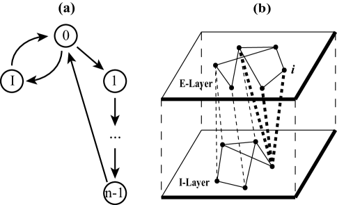
Figure 1: Illustrations of the state of excitable nodes and E-I layered network. (a) The state evolution of an excitable node. The symbol I represents the inhibited state. (b) A schema of a E-I network. The E-layer is consist of excitatory nodes while the I-layer only contains inhibitory nodes. The bold dotted lines are inhibitory paths of node $i$.

To analyze the dynamics of this system, we denote the probability that a given node $i$ is excited $(s=1)$ at time $t$ by $p_{i}^{t}$. In this model, we define the network instantaneous activity $p^{t}$ at time $t$ as the fraction of excited excitatory nodes, i.e. $p^{t}=\frac{1}{N_{e}}\sum_{i=1}^{N_{e}}p_{i}^{t}$. Notice that we only care about the excitatory nodes here. We also define the average activity $F=\frac{1}{T}\sum_{t=1}^{T}p^{t}$, where $T$ is a large time window. As a function of the stimulus intensity $\eta$, networks have a minimum response $F_{0}$ and a maximum response $F_{max}$. We define the dynamic range $\Delta=10\log(\eta_{high}/\eta_{low})$ as the range of stimuli that is distinguishable based on the system’s response $F$, discarding stimuli that are too weak to be distinguished from $F_{0}$ or too close to saturation. The range $[\eta_{low},\eta_{high}]$ is found from its corresponding response interval $[F_{low},F_{high}]$, where $F_{x}=F_{0}+x(F_{max}-F_{0})$. The choice of interval is arbitrary and does not affect our results.

In the following text, we will investigate this model on networks with various topologies. As typical examples of homogeneous and heterogeneous networks, random networks and scale-free networks will be analyzed separately.

III Random Networks

The network with $N$ nodes is an $Erd\ddot{o}s-R\acute{e}nyi$ (ER) undirected random graph, with $NK/2$ links being assigned to randomly chosen pairs of nodes. This produces an average degree $K$. We randomly choose $N_{e}=f_{e}N$ nodes as excitatory elements, and the rest as inhibitory ones. For simplicity, we set the strength of interactions between the nodes as $S$ uniformly. In a mean-field approximation, the average branching ratio KC of excitatory nodes $\sigma=KS$ corresponds to the average number of excitations created in the next time step by an excited excitatory element. Of all these excited nodes, $f_{e}\sigma$ nodes are excitatory and the others are inhibitory.

In the case of random networks, the update equations for both E-layer and I-layer are same. Assume that the events of neighbors of a node being excited at time $t$ are statistically independent. It is shown that this approximation yields good results even the network has a non-negligible amount of short loops LSR . Therefore, we obtain the following mean-field map for $p^{t}$ at sufficient long time $t$:

$$p^{t+1}=(1-(n-1)p^{t})(1-Sp^{t})^{f_{i}K}$$

$$\times\{\eta+(1-\eta)[1-(1-Sp^{t})^{f_{e}K}]\}.$$ (2)

In the stationary state, $p^{t+1}=p^{t}=p$. Thus $F=\frac{1}{T}\sum_{t=1}^{T}p^{t}\approx p$ for large $T$. To check the critical behavior without an external field, we set $\eta=0$ and linearize the term $(1-Sp^{t})^{f_{i}K}$ and $(1-Sp^{t})^{f_{e}K}$ in Eq.(2) around $p^{t}=0$, obtaining

$$p\approx(1-(n-1)p)(1-f_{i}\sigma p)f_{e}\sigma p.$$ (3)

Up to first order, we have the nonzero solution

$$p\approx\frac{\sigma-1/f_{e}}{\sigma(f_{i}\sigma+n-1)}.$$ (4)

Therefore, the critical point is $\sigma_{c}=\frac{1}{f_{e}}$, corresponding to the condition that the average number of excitations in E-layer caused by an excited node at each time step is exactly one. In particular, $\lim_{\eta\rightarrow 0}F=0$ if $\sigma<\sigma_{c}$ and $\lim_{\eta\rightarrow 0}F>0$ if $\sigma>\sigma_{c}$.

Next we will analyze the effect of a vanishing field at the critical point. In the limit of $p\rightarrow 0$, Eq.(2) can be approximated by

$$p=(1-(n-1)p)e^{-f_{i}\sigma p}\{\eta+(1-\eta)(1-e^{-f_{e}\sigma p})\}.$$ (5)

At the critical point $\sigma_{c}=1/f_{e}$, we expand Eq.(5) to second order in the case of $\eta\rightarrow 0$. Then we have

$$p\approx\sqrt{\frac{\eta}{\sigma+n-3/2}}.$$ (6)

Making use of Eq.(5), we can also predict the dynamic range. We can solve stimulus $\eta$ for any given response $F$. For a system with refractory time $n$, the maximal response $F_{max}=1/n$. Once we find $F_{0}$, $F_{low}$ can be obtained. Then we can get $\eta_{low}$ with Eq.(5). For $\eta_{high}$, Eq.(5) is invalid because it is only valid for $p\rightarrow 0$. In order to approximate $\eta_{high}$, we set $\eta_{high}$ to one. Therefore, we have

$$\Delta=-10\log[1-e^{f_{e}\sigma F_{low}}+\frac{F_{low}}{1-(n-1)F_{low}}e^{\sigma F_{low}}].$$ (7)

Now we check the critical point of phase transition via simulations. Fig.2 shows the relationship between response $F_{\eta\rightarrow 0}$ and branching ratio $\sigma$ for different excitatory proportions $f_{e}=0.6$, $0.8$ and $1$. The critical point of each situation is in accordance with the theoretical value, satisfying $\sigma_{c}=1/f_{e}$. Meanwhile, the behavior near the critical point is well captured by Eq.$(\ref{E4})$.

Figure 2: Response $F_{\eta\rightarrow 0}$ versus branching ratio $\sigma$ on ER random networks with $N=10^{4}$, $K=10$, and $n=5$. The solid lines are theoretical values and the symbols represent simulation results. Simulations with $f_{e}=0.6$, $0.8$ and $1$ are plotted with different symbols respectively. The arrows point to critical points of theoretical results.

Then we check the effect of a vanishing field on the system. The response curves from $\sigma=0$ to $2$ (in intervals of $0.25$) for $f_{e}=0.8$ are presented in Fig.3. The theoretical prediction of Eq.$(\ref{E5})$ fits the simulation data well. The phase transition occurs at $\sigma=1.25$. In critical regime, the power law exponent $m=1/2$, compatible with Eq.$(\ref{E6})$. Meanwhile, in subcritical regime, $m=1$. The inset of Fig.3 shows the critical state for different branching ratios. The theoretical lines from Eq.$(\ref{E6})$ agree with the simulations.

Figure 3: Response $F$ versus stimulus $\eta$ from $\sigma=0$ to $2$ in intervals of $0.25$ for $f_{e}=0.8$. The points represent simulation results on ER random networks with $N=10^{4}$, $K=10$, and $n=5$. The lines correspond to theoretical result from Eq.$(\ref{E5})$. The line segments show the power law exponent $m$. The inset presents the critical state of $\sigma=1$, $1.5$ and $2$. The lines are the results of Eq.$(\ref{E6})$.

Fig.4 shows the dynamic range for $f_{e}=0.5$ and $2/3$. As can be seen, dynamic range versus branching ratio is optimized at the critical point $\sigma_{c}=1/f_{e}$. In the subcritical region, sensitivity is enlarged because weak stimuli are amplified due to activity propagation among neighbors. Therefore, the dynamic range increases monotonically with $\sigma$. In the supercritical region, the response $F$, which is positive, masks the present of weak stimuli, decreasing dynamic range.

Figure 4: Dynamic range $\Delta$ versus branching ratio $\sigma$. The points represent simulation results on ER random networks with $N=10^{4}$, $K=10$, and $n=5$. The lines correspond to theoretical results from Eq.$(\ref{E7})$. (a), $f_{e}=0.5$, $\sigma_{c}=2$. (b), $f_{e}=2/3$, $\sigma_{c}=1.5$.

Although the mean-field analysis applies for ER random networks quiet well, it is powerless when tackle the study of heterogeneous networks, which are ubiquitous in practical complex systems. Thus in next section, we will mainly deal with the scale-free networks, especially, the $Barab\acute{a}si-Albert$ (BA) networks AB .

IV Scale-Free Networks

For networks with heterogeneous topology, we have to analyze each node separately. Assume the connectivity matrix is $A=\{A_{ij}\}_{N\times N}$. Then the update equation for $p_{i}^{t}$ is

$$p_{i}^{t+1}=(1-(n-1)p_{i}^{t})\prod_{j=N_{e}+1}^{N}(1-A_{ij}p_{j}^{t})$$

$$\times\{\eta+(1-\eta)[1-\prod_{j=1}^{N_{e}}(1-A_{ij}p_{j}^{t})]\},$$ (8)

To examine the critical point, we set $\eta=0$ and expand Eq.$(\ref{E8})$ to first order in the limit of $p_{i}^{t}\rightarrow 0$. We have

$$p_{i}^{t+1}=\sum_{j=1}^{N_{e}}A_{ij}p_{j}^{t}.$$ (9)

Based on matrix $A$, we create new matrices $A^{E}$ and $A^{I}$ as follows

$$A^{E}=\left(\begin{array}[]{cc}A^{EE}&\bm{0}\\ A^{EI}&\bm{0}\\ \end{array}\right),$$ (10)

$$A^{I}=\left(\begin{array}[]{cc}\bm{0}&A^{IE}\\ \bm{0}&A^{II}\\ \end{array}\right).$$ (11)

Thus, Eq.$(\ref{E9})$ can be transformed into

$$\bm{p}^{t+1}=A^{E}\bm{p}^{t},$$ (12)

where $\bm{p}^{t}=(p_{1}^{t},\cdots,p_{N}^{t})^{T}$ is the probability vector at time $t$. We can see the stability of the solution $\bm{p}=0$ is governed by the dominant eigenvalue $\lambda$ of matrix $A^{E}$. Therefore, the phase transition happens at $\lambda_{c}=1$. Notice that $A^{E}_{ij}\geq 0$, so $\lambda$ is real and positive according to Perron-Frobenius theorem M . Recall Eq.$(\ref{E10})$, $\lambda$ is in fact the dominant eigenvalue of matrix $A^{EE}$. This means that the critical point only determined by the topology of E-layer.

Relating Eq.$(\ref{E12})$ with the power method in numerical analysis, we find that for small $\bm{p}$ and $\eta$, $\bm{p}$ should be almost proportional to the normalized right eigenvector $\bm{u}$ of $A^{E}$ corresponding to $\lambda$. Thus we assume $p_{i}=Cu_{i}+\epsilon_{i}$ where $C$ is a constant and $\epsilon_{i}$ is an error term. Based on this, we obtain

$$F=\frac{1}{N_{e}}\sum_{i=1}^{N_{e}}p_{i}\approx\frac{1}{N_{e}}\sum_{i=0}^{N_{e}}Cu_{i}=C\langle u\rangle_{e}.$$ (13)

Here $\langle u\rangle_{e}=\sum_{i=1}^{N_{e}}u_{i}/N_{e}$. Near the critical state, we can approximate the product terms of Eq.$(\ref{E8})$ with exponential ones. Then in the steady state, we have

$$p_{i}=(1-(n-1)p_{i})\exp(-\sum_{j=N_{e}+1}^{N}A_{ij}p_{j})$$

$$\times\{\eta+(1-\eta)[1-\exp(-\sum_{j=1}^{Ne}A_{ij}p_{j})]\}.$$ (14)

To solve the stationary state, set $\eta=0$. Then using $p_{i}=Cu_{i}+\epsilon_{i}$ and $A^{E}\bm{u}=\lambda\bm{u}$, we expand Eq.$(\ref{E14})$ to second order for $p_{i}\rightarrow 0$.

$$Cu_{i}+\epsilon_{i}=(A^{E}\bm{\epsilon})_{i}+C\lambda u_{i}-C^{2}\lambda u_{i}(A^{I}\bm{u})_{i}$$

$$-((n-1)\lambda+\frac{1}{2}\lambda^{2})C^{2}u_{i}^{2}.$$ (15)

In order to eliminate the error term $\epsilon_{i}$, we make use of the left eigenvector $\bm{v}$ corresponding to $\lambda$ LSR . Recall Eq.$(\ref{E10})$ and $(\ref{E11})$, we can reveal more details about $\bm{u}$ and $\bm{v}$ and simplify the calculation. Assume the right and left eigenvector of $A^{EE}$ corresponding to the dominant eigenvalue $\lambda$ is $\bm{u}^{E}$ and $\bm{v}^{E}$ respectively. We can express $\bm{u}$ and $\bm{v}$ using $\bm{u}^{E}$ and $\bm{v}^{E}$:

$$\bm{u}=(\bm{u}^{E},\frac{1}{\lambda}A^{EI}\bm{u}^{E})^{T},\bm{v}=(\bm{v}^{E},\bm{0}).$$ (16)

We multiply Eq.$(\ref{E15})$ by $v_{i}$ and sum over $i$. Using that $\bm{v}A^{E}\bm{\epsilon}=\lambda\bm{v}\bm{\epsilon}$, we can neglect the term $(1-\lambda)\sum_{i}v_{i}\epsilon_{i}$ for $\lambda$ close to 1. Notice that $v_{i}=0$ for $N_{e}+1\leq i\leq N$. So in fact only the first $N_{e}$ equations exists. Thus, we divide the summation by $N_{e}$. With this equation, the constant $C$ can be easily solved. Therefore for $\eta=0$ the nonzero solution for $F$ is

$$F_{\eta=0}=\frac{(\lambda-1)\langle uv\rangle_{e}\langle u\rangle_{e}}{\lambda((n-1)+\frac{1}{2}\lambda)\langle u^{2}v\rangle_{e}+\langle u(A^{I}u)v\rangle_{e}},$$ (17)

where $\langle uv\rangle_{e}=\sum_{i=1}^{N_{e}}u_{i}v_{i}/N_{e}$, $\langle u^{2}v\rangle_{e}=\sum_{i=1}^{N_{e}}u_{i}^{2}v_{i}/N_{e}$, and $\langle u(A^{I}u)v\rangle_{e}=\frac{1}{N_{e}}\sum_{i=1}^{N_{e}}v_{i}u_{i}\sum_{k}\sum_{j}A_{ij}^{IE}A_{jk}^{EI}u_{k}$.

Figure 5: Response $F$ versus the dominant eigenvalue $\lambda$ of E-layer on BA scale-free networks with node number $N=10^{4}$, mean degree $\langle k\rangle=4$, and refractory time $n=2$. The points represent simulation results, whereas the lines correspond to the theoretical value from Eq.$(\ref{E17})$. (a), the fraction of excitatory nodes $f_{e}=0.6$.(b),the fraction of excitatory nodes $f_{e}=0.8$.

In order to test these theoretical results via simulations, we first created binary networks ($A_{ij}\in\{0,1\}$) with the $Barab\acute{a}si-Albert$ model. Then we calculate the largest eigenvalue $\lambda$ of the binary network and multiply $A$ by a constant to rescale the largest eigenvalue to the targeted one.

Fig.5 presents the relationship between response $F_{\eta\rightarrow 0}$ and the largest eigenvalue $\lambda$ for $f_{e}=0.6$ and $f_{e}=0.8$. For both cases, the criticality occurs at $\lambda_{c}=1$. And the behavior near critical point can be approximated by Eq.$(\ref{E17})$.

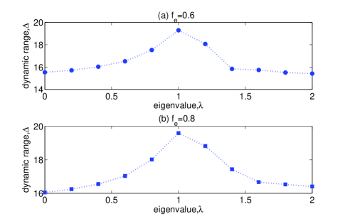
Figure 6: Dynamic range $\Delta$ versus the dominant eigenvalue $\lambda$ of E-layer on BA scale-free networks with node number $N=10^{4}$, mean degree $\langle k\rangle=4$, and refractory time $n=2$. The points represent simulation results. (a), the fraction of excitatory nodes $f_{e}=0.6$.(b),the proportion of fraction nodes $f_{e}=0.8$.

The maximal dynamic range is observed at criticality $\lambda_{c}=1$, see Fig.6. Just as the case of ER random networks, in the subcritical regime, dynamic range increases monotonically with the dominant eigenvalue $\lambda$ due to enhancement of link strength. On the contrary, in supercritical region, dynamic range decreases because of the increase of self-sustained activity $F$.

Relating to the result of ER random networks, assume the mean degree of E-layer is $\langle k\rangle_{e}$. Because the E-layer and I-layer are randomly connected, and the fraction of excitatory nodes is $f_{e}$, we have $\langle k\rangle_{e}=Kf_{e}$. In the case of ER random networks, the largest eigenvalue of $A^{EE}$ can be approximated by $\lambda\approx\langle d\rangle_{e}$, where $\langle d\rangle_{e}=\frac{1}{N_{e}}\sum_{i,j=1}^{N_{e}}A_{ij}^{EE}\approx S\langle k\rangle_{e}=\sigma f_{e}$. Then the critical point $\sigma_{c}$ satisfies $\sigma_{c}f_{e}=1$, which is identical to the result of Eq.$(\ref{E4})$.

In the next section, we will explore the way to further enhance dynamic range of a given network.

V Enhancing Dynamic Range of E-I Networks

In this section, we will explore the method to enhance dynamic range of E-I networks. Based on our analysis above, dynamic range is maximized at criticality. Therefore, it is trivial to adjust the link strength to make the system reach critical state. Then the question we face now is how to further improve dynamic range for a given network at criticality.

Now we give an analysis about the dynamic range at criticality. Since the dynamic range is maximized at criticality, we set $\lambda=1$ in Eq.$(\ref{E14})$. Then we can solve the stimulus level $\eta$ corresponding to the response $F$. To the first order, we obtain the rough result

$$\eta\approx\frac{(n-\frac{1}{2})\langle u^{2}v\rangle_{e}+\langle u(A^{I}u)v\rangle_{e}}{\langle v\rangle_{e}\langle u\rangle_{e}^{2}}F^{2}.$$ (18)

Here $\langle u^{2}v\rangle_{e}=\sum_{i=1}^{N_{e}}u_{i}^{2}v_{i}/N_{e}$ and $\langle u(A^{I}u)v\rangle_{e}=\frac{1}{N_{e}}\sum_{i=1}^{N_{e}}v_{i}u_{i}\sum_{k}\sum_{j}A_{ij}^{IE}A_{jk}^{EI}u_{k}$. The eigenvector $\bm{u}$ and $\bm{v}$ only relate to $A^{EE}$. Once $A^{EE}$ reaches critical state, $\bm{u}$ and $\bm{v}$ will be fixed. However, we can adjust the matrix $A^{I}$ to reduce the item $\langle u(A^{I}u)v\rangle_{e}$. Notice that, this procedure will not affect the critical state. Based on the definition of $\langle u(A^{I}u)v\rangle_{e}$, we define an inhibitory factor $\delta_{i}$ for each excitatory node $i$ as follows:

$$\delta_{i}=v_{i}u_{i}\sum_{k}\sum_{j}A_{ij}^{IE}A_{jk}^{EI}u_{k}.$$ (19)

We now explain the meaning of the inhibitory factor $\delta_{i}$. In the case of weak stimulus, the influence of inhibitory nodes is relatively passive. According to the rule, only the inhibitory nodes are activated can they release inhibitory signals. Thus in this condition, excitatory nodes actually have two effects: activating their excitatory neighbors to transmit excitations and inhibitory neighbors to release inhibitory signals. The later effect is implemented via the inhibitory paths, which start from excitatory nodes and end in E-layer through one step in I-layer, see Fig$\ref{illustration}(b)$. For the inhibitory paths which start at node $i$ and ends at node $k$, the interaction strength is $\sum_{j}A_{ij}^{IE}A_{jk}^{EI}$. Because in stationary state, excitatory nodes have different active probabilities, each inhibitory path should have its own weight. Here we set the weight as $u_{i}u_{k}$, reflecting the active probability of node $i$ and $k$. After summarizing the weighted interaction strength of inhibitory paths starting from node $i$, we have $u_{i}\sum_{k}\sum_{j}A_{ij}^{IE}A_{jk}^{EI}u_{k}$. Lastly, we multiply it with $v_{i}$ to reflect the active probability of node $i$, obtaining the definition of inhibitory factor $\delta_{i}$. Therefore, $\delta_{i}$ can be interpreted as the ability of node $i$ to cause inhibition in stationary state. In the procedure of enhancing dynamic range, we only need to cut out the nodes with large $\delta_{i}$ from I-layer.

Figure 7: Inhibitory factor $\delta_{i}$ versus node degree $k$. (a), simulation on ER random networks with node number $N=10^{4}$, mean degree $\langle k\rangle=10$, and $f_{e}=0.8$. (b), simulation on BA scale-free networks with node number $N=10^{4}$, mean degree $\langle k\rangle=4$, and $f_{e}=0.8$. The solid dots represent the mean values and the vertical lines show the standard deviations.

Now we check the relationship between the inhibitory factor and degree. In Fig.7 we present the simulation results of both ER random networks and BA scale-free networks. The solid dots represent the mean value and the vertical lines show the standard deviation. For ER random networks, nodes with small degree always have small $\delta_{i}$. However, for nodes with large degree, there are huge fluctuations in $\delta_{i}$. We quantify these fluctuations with standard deviations. As can be seen, the standard deviations are comparable with mean values, making the ranges of inhibitory factor for different degrees overlap with each other. More simulations with different network sizes show that these huge relative fluctuations also exist for other system sizes. As for scale-free networks, the values of $\delta_{i}$ are divided into two groups: for most nodes with small degree, their inhibitory factors are negligible; whereas, highly-connected nodes have larger $\delta_{i}$, which also shows great fluctuations. Also, these fluctuations are unrelated to system size. It can be seen there is no clear relations between inhibitory factor and degree. Consequently, it is unreasonable to just cut out the nodes with high degree from the I-layer.

We give an analysis of improvement of dynamic range. By Eq.$(\ref{E18})$ and definition of dynamic range, we have the upper bound on the improvement in dynamic range

$$\Delta_{u}=10\log(1+\frac{\langle u(A^{I}u)v\rangle_{e}}{(n-\frac{1}{2})\langle u^{2}v\rangle_{e}}).$$ (20)

For ER random networks, we can simplify the calculation as follows. For E-I networks with mean degree $K$, on average, each excitatory node has $f_{i}K$ edges pointing to I-layer, and each inhibitory node has $f_{e}K$ edges pointing back to E-layer. So we approximate $\sum_{j}A^{IE}_{ij}A^{EI}_{jk}\approx f_{i}KS\cdot f_{e}KS/N_{e}$. Substituting this term in Eq.$(\ref{E19})$, we have

$$\delta_{i}\approx v_{i}u_{i}f_{e}f_{i}K^{2}S^{2}\langle u\rangle_{e}.$$ (21)

Then we use Eq.$(\ref{E20})$ to obtain

$$\Delta_{u}=10\log(1+\frac{f_{e}f_{i}K^{2}S^{2}\langle u\rangle_{e}}{N_{e}(n-1/2)\langle u^{2}v\rangle_{e}}).$$ (22)

As for scale-free networks, we can check the upper bound through numerical calculations.

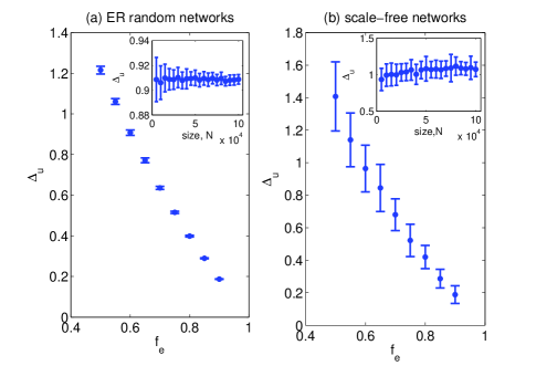
Figure 8: Upper bound $\Delta_{u}$ versus $f_{e}$. Networks are at critical state. The solid dots are mean values and vertical lines show standard deviations. (a), simulation on ER random networks with node number $N=10^{4}$, mean degree $\langle k\rangle=20$, and $f_{e}=0.6$. (b), simulation on BA scale-free networks with node number $N=10^{4}$, mean degree $\langle k\rangle=4$, and $f_{e}=0.6$. Insets show the relationship between $\Delta_{u}$ and system size $N$ for each case.

Fig.8 shows the simulations of upper bound $\Delta_{u}$. For both cases, $\Delta_{u}$ decreases with the increasing fraction of excitatory nodes $f_{e}$. The only difference is that scale-free networks present larger fluctuation, which cannot affect the decreasing trend. In the insets, we explore the effect of system size on upper bound. It can be seen for both cases, $\Delta_{u}$ is not influenced by system size. Also, the scale-free networks show larger fluctuation. Another conclusion we get from Fig.8 is that the improvement is small compared to the original dynamic range. This can be explained as follows. Firstly, $A^{IE}$ and $A^{EI}$ are sparse, so there are not much inhibitory paths exist. This makes the term $\sum_{j}A^{IE}_{ij}A^{EI}_{jk}$ very small. Therefore, by Eq.$(\ref{E19})$ and $(\ref{E20})$, $1+\frac{\langle u(A^{I}u)v\rangle_{e}}{(n-\frac{1}{2})\langle u^{2}v\rangle_{e}}$ is close to $1$, which makes $\Delta_{u}$ small. Secondly, in the critical state, each excitatory node can only excite a small number of inhibitory nodes. Because the function of inhibitory nodes is passive (i.e. only they are excited can they exert inhibitory impact), this weakens the influence of inhibitory nodes. Consequently, cutting out the inhibitory nodes can only enhance dynamic range a little. In fact, by this method, we cannot change the functional form $\eta\propto F^{2}$. We can only change the constant parameter.

To check the effect of our method, we perform a comparison of random remove and targeted remove. Denote $p_{r}$ as the fraction of nodes which are cut out from I-layer. In random remove, we choose the nodes randomly, while in targeted remove we select the nodes with top $p_{r}$ percent inhibitory factors. In Fig.9, we can see for both cases, dynamic range of targeted remove increases faster than that of random remove. However, the improvement is relatively small compared with the original dynamic range.

Figure 9: Dynamic range $\Delta$ versus remove probability $p_{r}$ for random remove and targeted remove. The networks are at critical state. Data in two cases are displayed with different symbols. (a), simulation on ER random networks with node number $N=10^{4}$, mean degree $\langle k\rangle=20$, and $f_{e}=0.6$. (b), simulation on BA scale-free networks with node number $N=10^{4}$, mean degree $\langle k\rangle=4$, and $f_{e}=0.6$. The red line is the upper bound of improvement.

VI Conclusions and Discussions

In this paper, we propose an excitatory-inhibitory excitable network model. To analysis the criticality and dynamic range of this model, we divide this network into two layers: E-layer which consist of excitatory nodes and I-Layer which only contains inhibitory ones. Based on it, we give a theoretical analysis on random networks and scale-free networks respectively. It is proved that, the critical state occurs at $\sigma_{c}=1/f_{e}$ for random networks and the dynamic range is maximized at criticality. As for scale-free networks, the phase transition happens when the largest eigenvalue of the E-layer’s weighted adjacency matrix $A^{EE}$ is just one. Similarly, the dynamic range is also optimized at critical point. It is interesting that the critical point is not affected by the I-layer and the links between these two layers. Then, we discuss the method to enhance dynamic range. Based on the analysis of mutual effects, we propose an inhibitory factor $\delta_{i}$ for each excitatory node to quantify their inhibitory ability. By cutting out the excitatory nodes with high inhibitory ability from I-Layer, the dynamic range can be further improved. However, the improvement is relatively small. We give an analysis to the upper bound on improvement in dynamic range and explain why the enhancement is small.

For further study, it is meaningful to investigate networks with heterogenous connectivity strength GHI . Meanwhile, the study of real-world neural or sensor networks is also of great significance for the applications of the theory.

- (1) D.J. Watts and S.H. Strogatz, Nature (London) 393, 440 (1998).
- (2) R. Albert and A.L. Barabási, Science 286, 509 (1999).
- (3) O. Kinouchi and M. Copelli, Nat. Phys. 2, 348 (2008).
- (4) E. Bullmore and O. Sporns, Nature (London) 10, 186 (2009).
- (5) R. Pastor-Satorras and A. Vespignani, Phys. Rev. Lett. 86, 3200 (2001).
- (6) C. Castellano, S. Fortunato, and V. Loreto, Rev. Mod. Phys. 81, 2, (2009).
- (7) V.M. Yakovenko and J.B. Rosser Jr., Rev. Mod. Phys. 81, 1703 (2009).
- (8) S. Pei, S. Tang, X. Zhang, Z. Liu, and Z. Zheng, Physica A 391, 2023, (2012).
- (9) J.M. Beggs and D. Plenz, J. Neurosci 23, 11167, (2003).
- (10) J.M. Beggs and D. Plenz, J. Neurosci 22, 5216, (2004).
- (11) J. Soriano, M.R. Martinez, T. Tlusty, and E. Moses, Proc. Natl. Acad. Sci. USA 105, 13758, (2008).
- (12) I. Breskin, J. Soriano, E. Moses, and T. Tlusty, Phys. Rev. Lett. 97, 188102 (2006).
- (13) D.H. Zanette and M. Kuperman, Physica A 309, 445 (2002).
- (14) L.M. Fernández-Carrasco, H. Terashima-Marín, and M. Valenzuela-Rendón, IEEE International Conference on Systems, Man and Cybernetics, 1181 (2008).
- (15) M. Copelli, A.C. Roque, R.F. Oliveira, and O. Kinouchi, Phys. Rev. E 65, 060901 (2002).
- (16) M. Copelli, R.F. Oliveira, A.C. Roque, and O. Kinouchi, Neurocomputing, 65, 691 (2005).
- (17) M. Copelli and P.R.A. Campos, Eur. Phys. J. B 56, 273 (2007).
- (18) A.C. Wu, X.J. Xu, and Y.H. Wang, Phys. Rev. E 75, 032901 (2007).
- (19) D.B. Larremore, W.L. Shew, and J.G. Restrepo, Phys. Rev. Lett. 106, 058101 (2011).
- (20) D.B. Larremore, W.L. Shew, E. Ott, and J.G. Restrepo, Chaos 21, 025117 (2011).
- (21) Y. Adini, D. Sagi, and M. Tsodyks, Proc. Natl. Acad. Sci. U.S.A. 94, 10426 (1997).
- (22) C. Park and D. Terman, Chaos 20, 023122 (2010).
- (23) T.P. Vogels, K. Rajan, and L.F. Abbott, Annu. Rev. Neurosci. 28, 357 (2005).
- (24) S.E. Folias and G.B. Ermentrout, Phys. Rev. Lett. 107, 228103 (2011).
- (25) V. Litvak, H. Sompolinsky, I. Segev, and M. Abeles, J. Neurosci. 7, 3006 (2003).
- (26) M.N. Shadlen and W.T. Newsom, Curr. Opin. Neurobiol. 4, 569 (1994).
- (27) J. Kremkow, A. Aertsen, and A Kumar, J. Neurosci. 47, 15760 (2010).
- (28) T.P. Vogels and L.F. Abbott, Nat. Neurosci. 12, 483 (2009).
- (29) M.N. Shadlen and W.T. Newsome, J. Neurosci. 10, 3870 (1999).
- (30) N. Brunel, J. Comput. Neurosci. 8, 183 (2000).
- (31) M. Okun and I. Lampl, Nat. Neurosci. 11, 535 (2008).
- (32) W.B. Wilent and D. Contreras, Nat. Neurosci. 8, 1364 (2005).
- (33) M. Kurant and P. Thiran, Phys. Rev. Lett. 96, 138701 (2006).
- (34) C.R. MacCluer, SIAM Rev. 42, 487 (2000).
- (35) C.V. Giuraniuc, J.P.L. Hatchett, J.O. Indekeu, M. Leone, I. Pérez Castillo, B. Van Schaeybroeck, and C. Vanderzande, Phys. Rev. Lett. 95, 098701 (2005).