Information-based measure of nonlocality

Abstract

Quantum nonlocality concerns correlations among spatially separated systems that cannot be explained classically without communication among the parties. Thus, a natural measure of nonlocal correlations is provided by the minimal amount of communication required for classically simulating them. In this paper, we present a method to compute the minimal communication cost of parallel simulations, which we call nonlocal capacity, for any general nonsignaling correlations. This measure turns out to have an important role in communication complexity and can be used to discriminate between local and nonlocal correlations, as an alternative to the violation of Bell’s inequalities.

I Introduction

The outcomes of measurements performed on spatially separate entangled systems can display nonlocal correlations that cannot be explained classically without some communication bell . In particular, one of the parties needs some information on the measurement choice of the other party. These nonlocal correlations can be used as an information-theoretic resource. For example, they can exponentially reduce the amount of communication required to solve some distributed computational problems cleve ; buhrman . Furthermore, for some tasks, the use of nonlocal correlations can make communication unnecessary, such as in pseudo-telepathy games brassard . Some stronger-than-quantum nonsignaling correlations can even collapse the communication complexity in any two-party scenario. Indeed, the access to an unlimited number of Popescu-Rohrlich (PR) nonlocal boxes allows two parties to solve any communication complexity problem with the aid of a constant amount of classical communication vandam . Nonlocal correlations have also a fundamental role in device-independent applications, such as key agreement in cryptography barrett0 ; acin0 ; scarani ; acin2 ; acin3 ; masanes ; hanggi and randomness amplification colbeck ; gallego .

As the violation of a given Bell inequality is the signature of nonlocal correlations, a possible measure of nonlocality is the strength of this violation. However, since this quantity has no obvious relation with information, it does not necessarily provide a reliable measure as an information-theoretic resource. A more natural measure has been employed in Refs. maudlin ; brassard ; steiner ; gisin1 ; gisin2 and relies on the very definition of nonlocality; nonlocal correlations require some communication to be classically simulated, thus the minimal amount of required classical communication can be used as a measure of the strength of nonlocality. This measure, which we call communication complexity of the nonlocal resource, provides an ultimate limit to the power of nonlocal correlations in terms of classical communication in a two-party scenario. Indeed, nonlocal resources cannot replace an amount of classical communication bigger than the associated communication complexity. As shown in Ref. pironio , the strength of the Bell inequality violation and the communication complexity of nonlocal resources turn out to be identical if the average amount of communication is employed as measure of the communication cost and the optimal inequality is taken for the given nonlocal correlations. In this paper, we mainly focus on the minimal asymptotic communication cost of parallel simulations in the asymptotic limit of infinite instances. This quantity, which we call nonlocal capacity, turns out to be much easier to be computed than its single-shot counterpart. Furthermore, tight lower and upper bounds on the minimal average communication cost are given in terms of the nonlocal capacity, as discussed later. Thus, the nonlocal capacity also gives tight bounds on the maximal violation of the Bell inequalities. Alternative measures of nonlocality could use different resources as unit of nonlocality, such as nonlocal boxes barrett ; brunner . For example, the strength of nonlocality could be defined as the number of PR-boxes necessary to simulate the correlations. However, no finite set of PR-boxes can simulate all bipartite nonlocal correlations dupuis ; wolf .

By definition, the computation of the nonlocal capacity is an optimization problem, but it is not convex in its original form. This makes it very hard to find the global minimum, expecially when the set of allowed measurements is large. In this paper, we show that the problem can be reduced to a convex minimization problem, which can be numerically solved with very efficient algorithms boyd . Then, we discuss the relation with a previous work on the communication complexity of channels in general probabilistic theories montina1 . Finally, we illustrate the method with a numerical example.

II Communication cost of nonlocal correlations

Figure 1: (a) Nonsignaling box with inputs $a$ and $b$ and outcomes $r$ and $s$. (b) Simulation of the nonsignaling box through shared stochastic variable $y$ and communication of the variable $k$.

In this paper, we will discuss the general case of nonsignaling correlations, which satisfy the minimal requirements of relativity and causality. Namely, the object that we will consider is a nonsignaling box, which is an abstract generalization of the following quantum scenario. Two parties, say Alice and Bob, simultaneously perform a measurement on two spatially separate parts of an entangled system. In general, Alice and Bob are allowed to choose among their respective sets of possible measurements. We assume that Bob’s set of measurements is finite, but arbitrarily large. For the sake of simplicity, we also assume that Alice’s set is discrete, although this is not strictly necessary. Let us denote by the indices $a$ and $b$ the measurements performed by Alice and Bob, respectively. The index $b$ takes a value in $\{1,\dots,M\}$, where $M$ is the number of measurements that Bob can perform. After the measurements, Alice gets an outcome $r$ and Bob an outcome $s$. The overall scenario is described by the joint conditional probability $P(r,s|a,b)$. This distribution satisfies the nonsignaling conditions

$$\begin{array}[]{c}\sum_{s}P(r,s|a,b)=\sum_{s}P(r,s|a,\bar{b})\equiv P(r|a)\;\forall a,b,\bar{b},r,\vspace{1mm}\\ \sum_{r}P(r,s|a,b)=\sum_{r}P(r,s|\bar{a},b)\equiv P(s|b)\;\forall a,\bar{a},b,s.\end{array}$$ (1)

These conditions are implied by causality and relativity. In the following discussion, we consider a more general scenario including non-quantum correlations and we just assume that the joint conditional probability satisfies the nonsignaling condition. The abstract machine producing the correlated variables $r$ and $s$ from the inputs $a$ and $b$ will be called nonsignaling box (briefly, NS-box). The NS-box, schematically represented in Fig. 1a, is identified with the conditional probability $P(r,s|a,b)$.

In general, a classical simulation of the joint distribution $P(r,s|a,b)$ requires some communication between the parties. We assume that only a one-way communication from Alice to Bob is allowed. The classical protocol is as follows (as illustrated in Fig. 1b). Alice generates an outcome $r$ and a variable $k$ with probability $P(k,r|y\,a)$ depending on the variable $a$ and some stochastic variable $y$ shared with Bob and generated with probability $\rho(y)$. The variable $k$ is sent to Bob. Finally, Bob generates an outcome $s$ with probability $P(s|y\,b\,k)$ depending on $y$, $b$ and $k$. The protocol simulates the NS-box $P(r,s|a,b)$ if

$$\sum_{k}\int dyP(s|y\,b\,k)P(k,r|y\,a)\rho(y)=P(r,s|a,b).$$ (2)

We define the communication complexity (denoted by ${\cal C}_{nl}$) of the NS-box as the minimal amount of communication $\cal C$ required for an exact simulation of the NS-box.

There are different measures of amount of communication. Here we employ the entropic definition, although the presented results apply also to the case of average communication. Let us introduce the conditional probability

$$P(k|y)\equiv\sum_{r,a}P(k,r|y,a)P(a)$$

and the corresponding conditional Shannon entropy of the variable $K$ given $Y$

$$H_{P(a)}(K|Y)\equiv-\int dy\rho(y)\sum_{k}P(k|y)\log_{2}P(k|y),$$

which depends on $P(a)$. We define the communication cost $\cal C$ of the simulation as the maximum, over the space of distributions $P(a)$, of $H_{P(a)}(K|Y)$, that is,

$${\cal C}\equiv\max_{P(a)}H_{P(a)}(K|Y)$$ (3)

(see also Refs. montina1 ; montina2 and later discussion for the operational interpretation). Note the abuse of notation in Eq. (3). The maximization is performed with the respect to $P(a)$ as a function of $a$. The argument of the function $P(a)$ is used to distinguish it from the other distributions, such as $P(s|y\,b\,k)$ and $P(k,r|y\,a)$. The same representation is used for the label of $H_{P(a)}(K|Y)$. For the sake of simplicity, we will use this notation whenever the meaning is clear from the context.

The operational interpretation of $\cal C$ is provided by Shannon’s source coding theorem and the wrong code theorem (Theorem 5.4.3 in Ref. cover ). Given a compression code for $k$, let us denote by $L(a)$ the expected length of the codeword of $k$ for a given input $a$ and by $\bar{L}[P(a)]\equiv\sum_{a}P(a)L(a)$ the expected length averaged over $a$ with the distribution $P(a)$. The interpretation of $\cal C$ is given by the following properties. There is an optimal coding such that the minimal worst-case expected length $\max_{a}L(a)$ is equal to $\cal C$ up to one additional bit, that is,

$${\cal C}\leq\max_{a}L(a)\leq{\cal C}+1.$$ (4)

In other words, for the optimal code, Alice needs to send not more than ${\cal C}+1$ on average for every choice of the input $a$ and this bound is strict for some input $a$ up to one bit. Furthermore, the optimal code minimizing $\max_{a}L(a)$ also minimizes $\bar{L}[P(a)]$ for the worst-case distribution $P(a)$ and the minimum is equal to $\cal C$ up to one bit. It is worth to stress that the upper bound collapses to $\cal C$ if block-coding of $k$ is employed, as discussed later. Let us prove Ineqs. (4). Suppose that Alice and Bob employ the optimal code minimizing $\max_{a}L(a)$ and Alice chooses the input $a$ according to the distribution $P(a)$ maximizing $H_{P(a)}(K|Y)$, denoted by $P_{M}(a)$. From Shannon’s source coding theorem, we have that the expected length of the codeword of $k$, $\sum_{a}P_{M}(a)L(a)$, is not smaller than ${\cal C}=H_{P_{M}(a)}(K|Y)$. Thus,

$${\cal C}\leq\max_{a}L(a).$$ (5)

Let us define the distribution

$$P_{M}(k|y)\equiv\sum_{r,a}P(k,r|y,a)P_{M}(a).$$ (6)

From Shannon’s theorem, it is clear that the optimal code minimizing $\bar{L}[P(a)]$ for the worst-case distribution $P(a)$ is the code that minimizes $\bar{L}[P_{M}(a)]$ and the minimum is equal to $\cal C$ up to one bit. Now, we show that the optimal code minimizing $\bar{L}[P_{M}(a)]$ also minimizes $\max_{a}L(a)$ up to one additional bit. Namely, employing the optimal code for $P_{M}(a)$, the wrong code theorem implies that $\max_{a}L(a)$ is not bigger than ${\cal C}+1$. Indeed, if Alice generates $a$ according to a different distribution $P(a)$ and uses the code that is optimal for $P_{M}(a)$, the expected codeword length $\bar{L}[P(a)]$ is equal to the Shannon entropy $H_{P(a)}(K|Y)$ plus the relative entropy $D[P(k|y)||P_{M}(k|y)]$ up to an additional bit cover , where the relative entropy is cover

$$D[P(k|y)||P_{M}(k|y)]\equiv-\int dy\rho(y)\sum_{k}P(k|y)\log\frac{P(k|y)}{P_{M}(k|y)}.$$ (7)

Thus, defining the quantity

$$\begin{array}[]{c}{\cal C}[P(a)]\equiv H_{P(a)}(K|Y)+D[P(k|y)||P_{M}(k|y)]=\vspace{1mm}\\ -\int dy\rho(y)P(k|y)\log P_{M}(k|y),\end{array}$$ (8)

we have that

$$\bar{L}[P(a)]\leq{\cal C}[P(a)]+1.$$ (9)

Let us prove that

$${\cal C}[P(a)]\leq{\cal C}.$$ (10)

Given the distribution $P_{\alpha}(a)\equiv\alpha P(a)+(1-\alpha)P_{M}(a)$ with $\alpha\in[0,1]$, we have that

$$\left.\frac{dH_{P_{\alpha}(a)}(K|Y)}{d\alpha}\right|_{\alpha=0}\leq 0,$$ (11)

as $P_{M}(a)$ maximizes the conditional entropy. This equation implies Eq. (10), which can be seen by explicitly performing the derivation of the conditional entropy. Thus, from Eqs. (9,10), we have that $\bar{L}[P(a)]\leq{\cal C}+1$. Since this inequality holds for every $P(a)$, we have that $L(a)\leq{\cal C}+1$.

Figure 2: (a) $N$ identical nonsignaling boxes. On one side, Alices chooses the inputs $(a^{1},\dots,a^{N})$ and gets the outcomes $(r^{1},\dots,r^{N})$. On the other side, Bob chooses the inputs $(b^{1},\dots,b^{N})$ and gets the outcomes $(s^{1},\dots,s^{N})$. (b) Simulation of the $N$ nonsignaling boxes through a shared stochastic variable $y$ and the communication of the variable $k$.

If block-coding of many parallel instances of $k$ is employed, the minimal expected length $L(a)$ per instance turns out to be equal to $\cal C$ in the asymptotic limit of infinite instances. However, block-coding of $k$ is not the most general compression method in the case of a parallel simulation of NS-boxes. A more general protocol simulating $N$ NS-boxes, which is schematically represented in Fig. 2a, is as follows. The $i$th box has input $a^{i}$ and outcome $r^{i}$ on one side (Alice side), and input $b^{i}$ and outcome $s^{i}$ on the other side (Bob side). Alice chooses the input $(a^{1},\dots,a^{N})\equiv\vec{a}$ and gets the outcome $(r^{1},\dots,r^{N})\equiv\vec{r}$. Similarly, Bob chooses the input $(b^{1},\dots,b^{N})\equiv\vec{b}$ and gets the outcome $(s^{1},\dots,s^{N})\equiv\vec{s}$. Hereafter, we always use a superscript as a label of the NS-boxes. The parallel simulation of $N$ NS-boxes is the same as for a single box, with $a$, $b$, $r$ and $s$ replaced by $\vec{a}$, $\vec{b}$, $\vec{r}$ and $\vec{s}$. This more general scheme produces a global variable $k$ with a probability depending on the overall input $\vec{a}$. The protocol exactly simulates the $N$ boxes if

$$\sum_{k}\int dyP(\vec{s}|y\,\vec{b}\,k)P(k,\vec{r}|y\,\vec{a})\rho(y)=\prod_{i}P(r^{i},s^{i}|a^{i},b^{i}).$$ (12)

Each parallelized protocol has $N$ as a free parameter. The asymptotic communication cost of the protocol is defined as $\lim_{N\rightarrow\infty}{\cal C}^{par}/N\equiv{\cal C}^{asym}$, where ${\cal C}^{par}$ is the communication cost of the parallelized simulation. In this case, the maximization in Eq. (3) is performed over the space of joint input distributions $P(a_{1}\dots a_{N})$. We define the nonlocal capacity of the NS-box as the minimum of ${\cal C}^{asym}$ among the parallelized protocols. The nonlocal capacity is denoted by ${\cal C}_{nl}^{asym}$.

III Computation of nonlocal capacity as a convex optimization problem

Our task is to reduce the computation of ${\cal C}_{nl}^{asym}$ to the minimization of a functional over a suitable space of distributions. Let us define this space.
Definition 1. Given a nonsignaling box with conditional probability $P(r,s|a,b)$, the set ${\cal V}$ contains any conditional probability $\rho(r\,{\bf s}|a)$ over $r$ and the sequence ${\bf s}=(s_{1},\dots,s_{M})$ whose marginal distribution of $r$ and the $m$-th variable is the distribution $P(r,s|a,b=m)$. In other words, the set ${\cal V}$ contains any $\rho(r\,{\bf s}|a)$ satisfying the constraints

$$\sum_{{\bf s},s_{m}=s}\rho(r\,{\bf s}|a)=P(r,s|a,b=m),$$ (13)

where the summation is over every index in $\bf s$ except the $m$-th one, which is set equal to $s$. The subscript “${\bf s},s_{m}=s$” means that the summation is done over $\vec{s}$ with the constraint that the component $s_{m}$ is taken equal to $s$, that is,

$$\sum_{{\bf s},s_{m}=s}=\sum_{{\bf s}}\delta_{s_{m},s},$$ (14)

$\delta_{a,b}$ being the Kronecker delta.

The set $\cal V$ is surely non-empty. Indeed, the distribution $\rho(r\,{\bf s}|a)=P(s_{1}|r\,a\,b=1)\times\dots\times P(s_{M}|r\,a\,b=M)P(r|a)$ is an element of ${\cal V}$. Note that $\rho(r\,{\bf s}|a)$ can be defined only if the first nonsignaling condition (1) is satisfied. The conditional probability $\rho(r\,{\bf s}|a)$ defines a new box with a single input, $a$. We call this box ‘HV-box’, where HV stands for ‘hidden variable’. Indeed, this box gives simultaneously the outcomes for every query $b$ of Bob, whereas this information is partially hidden in a query of the original NS-box.

There is a trivial protocol that simulates a NS-box through its HV-box. Using the same terminology introduced in Ref. montina1 in the context of channels, we introduce the following protocol (Fig. 3a) that simulates a NS-box through one of its HV-boxes.
Master protocol. Alice generates the outcome $r$ and the array $\bf s$ according to a conditional probability $\rho(r\,{\bf s}|a)\in{\cal V}$. Then, she sends $\bf s$ to Bob. Finally, Bob chooses the input $b$ and gives the outcome $s=s_{b}$.
It is obvious that $r$ and $s$ are generated according to the conditional probability $P(r,s|a,b)$.

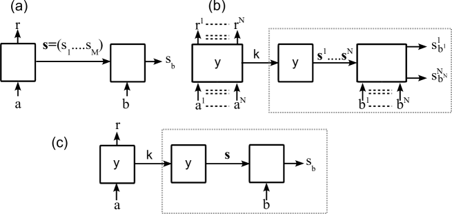
Figure 3: (a) Master protocol using a HV-box $\rho(r,{\bf s}|a)\in{\cal V}$ for simulating a NS-box. Alice sends $\bf s$, generated according to $\rho(r,{\bf s}|a)\in{\cal V}$. Bob generates the outcome $s_{b}$. (b) Child protocol using the simulation of $N$ HV-boxes by employing shared randomness and communication. First, $N$ identical HV-boxes $\rho(r^{1},{\bf s}^{1}|a^{1}),\dots,\rho(r^{N},{\bf s}^{N}|a^{N})\in{\cal V}$ are simulated as follows. Alice, who chooses $a^{1},\dots,a^{N}$ and generates $r^{1},\dots,r^{N}$, sends $k$, enabling Bob to generate the variables ${\bf s}^{1},\dots,{\bf s}^{N}$ of $N$ instances according to the distributions $\rho(r^{i},{\bf s}^{i}|a^{i})\in\cal V$. The two parties share the random variable $y$. Finally, Bob generates the outcomes $s^{1}_{b^{1}},\dots,s^{N}_{b^{N}}$, as done in the master protocol for a single instance. (c) One-shot child protocol. A single HV-box is simulated.

Through the procedure discussed in Ref. montina and used in Ref. montina1 for quantum channels, we show that it is possible to turn the master protocol into a child protocol (Fig. 3b) for parallel simulations whose asymptotic communication cost is the capacity of the channel $a\rightarrow{\bf s}$ associated to the conditional probability $\rho({\bf s}|a)\equiv\sum_{r}\rho(r\,{\bf s}|a)$. Let us recall that a channel $x_{1}\rightarrow x_{2}$ is identified by a conditional probability distribution $\rho(x_{2}|x_{1})$ and its capacity is the maximum of the mutual information between $x_{1}$ and $x_{2}$ over the space of probability distributions $\rho(x_{1})$ cover . Let us denote by $C(x_{1}\rightarrow x_{2})$ the capacity of the channel $x_{1}\rightarrow x_{2}$. The procedure in Ref. montina is based on the Reverse Shannon theorem rev_s . Using the single-shot version of the reverse Shannon theorem harsha , we also show that there is a single-shot simulation of a NS-box (Fig. 3c), with associated HV-box $\rho(r,{\bf s}|a)$, whose communication cost is equal to $C(a\rightarrow{\bf s})$ plus an additional term scaling as $\log C(a\rightarrow{\bf s})$.

Let us first prove the following.
Lemma 1. Multiple instances of identical HV-boxes $\rho(r,{\bf s}|a)$ can be simulated in parallel through local randomness and communication with asymptotic communication cost ${\cal C}^{asym}$ equal to the capacity of the channel $\rho({\bf s}|a)\equiv\sum_{r}\rho(r\,{\bf s}|a)$. That is,

$${\cal C}^{asym}=C(a\rightarrow{\bf s})$$ (15)

The communication is established from Alice to Bob. Alice chooses an input $a^{i}$ and gets an outcome $r^{i}$ in each instance $i$, whereas Bob gets the outcomes ${\bf s}^{i}$. The two parties can use shared random variables. Furthermore, there is a single-shot simulation of a HV-box with communication cost $\cal C$ such that

$${\cal C}^{asym}\leq{\cal C}\leq{\cal C}^{asym}+2\log_{2}[{\cal C}^{asym}+1]+2\log_{2}e.$$ (16)

Proof. The simulation is as follows. The $i$th instance has input $a^{i}$ and outcome $r^{i}$ on Alice’s side, and outcome ${\bf s}^{i}$ on Bob’s side. The outcomes are generated with conditional probability $\rho(r^{i},{\bf s}^{i}|a^{i})$. Alice chooses the inputs $a^{1},\dots,a^{N}$. Then she sends Bob an amount of information that allows Bob to generate the variables ${\bf s}^{1},\dots,{\bf s}^{N}$ according to the conditional probability $\rho({\bf s}^{i}|a^{i})$. The reverse Shannon theorem rev_s states that there is a protocol for this task with asymptotic communication cost equal to the capacity of the channel $\rho({\bf s}|a)$, provided that Alice and Bob share some stochastic variable, say $\chi$. It is always possible to have a deterministic protocol, so that the outcomes ${\bf s}^{1},\dots,{\bf s}^{N}$ are uniquely determined by $\chi$ and the communicated information. Since $\chi$ is shared with Alice, Alice knows Bob’s outcomes. Thus, Alice generates her outcomes $r^{1},\dots,r^{N}$ according to the conditional probability $\rho(r^{i}|a^{i}\,{\bf s}^{i})\equiv\rho(r^{i}\,{\bf s}^{i}|a^{i})/\rho({\bf s}^{i}|a^{i})$. The overall set of outcomes is generated according to the joint distribution $\rho(r^{i},{\bf s}^{i}|a^{i})$. The last statement of the lemma has a similar proof and uses the result in Ref. harsha . The single-shot version of the reverse Shannon theorem proved in Ref. harsha states that a single-shot simulation of the channel $a\rightarrow{\bf s}$ can be performed with a communication cost $\cal C$ satisfying the inequalities (16). $\square$
Lemma 1 directly implies the following.
Lemma 2. Identical NS-boxes can be simulated in parallel with an asymptotic communication cost ${\cal C}^{asym}$ equal to the capacity of the channel $\rho({\bf s}|a)\equiv\sum_{r}\rho(r\,{\bf s}|a)$, where $\rho(r\,{\bf s}|a)\in{\cal V}$ is an associated HV-box. The parallel protocol is obtained by using a parallel simulation of HV-boxes that employs shared randomness and communication. The overall protocol, called child protocol, is represented in Fig. 3b. Furthermore, there is a single-shot simulation of a NS-box with communication cost $\cal C$ satisfying the inequalities (16) (Fig. 3c).
Proof. This is a trivial consequence of Lemma 1. Indeed, a NS-box $P(r,s|a,b)$ can be simulated by a master protocol through an associated HV-box $\rho(r,{\bf s}|a)$, which can be simulated with asymptotic communication cost equal to the capacity of the channel $\rho({\bf s}|a)$ and with single-shot communication cost $\cal C$ satisfying constraints (16). $\square$

Let us define the quantity

$${\cal D}\equiv\min_{\rho(r,{\bf s}|a)\in{\cal V}}\max_{P(a)}I({\bf S};A)\equiv\min_{\rho(r,{\bf s}|a)\in{\cal V}}C(a\rightarrow{\bf s})$$ (17)

associated to a NS-box $P(r,s|a,b)$, where $I({\bf S};A)$ is the mutual information between the stochastic variables $\bf s$ and $a$ and $C(a\rightarrow{\bf s})$ the capacity of the channel $\rho({\bf s}|a)\equiv\sum_{r}\rho(r,{\bf s}|a)$. Clearly, $\cal D$ is the minimum of the capacity of the channels $a\rightarrow{\bf s}$ that are the marginals of the channels $a\rightarrow r,{\bf s}$ in the set $\cal V$. Lemma 2 implies that the nonlocal capacity of the NS-box $P(r,s|a,b)$ satisfies the inequality

$${\cal C}_{nl}^{asym}\leq{\cal D}.$$ (18)

The next main task is to prove that the optimal parallel protocol simulating identical NS-boxes is given by a child protocol (schematized in Fig. 3b) employing a simulation of parallel HV-boxes. The proof is a consequence of the data-processing inequality cover , which implies that ${\cal C}_{nl}^{asym}\geq\cal D$, and therefore

$${\cal C}_{nl}^{asym}={\cal D}.$$ (19)

Let us first consider a similar proof for the single-shot case, which is less intricate and elucidates the key ideas used in the proof of the main theorem. Namely, we show that ${\cal C}_{nl}\geq{\cal D}$.
Theorem 1. The communication complexity ${\cal C}_{nl}$ of a NS-box $P(r,s|a,b)$ satisfies the bounds

$${\cal D}\leq{\cal C}_{nl}\leq{\cal D}+2\log_{2}({\cal D}+1)+2\log_{2}e.$$ (20)

In few words, the procedure used in the proof of the Theorem 1 is as follows. Given an optimal protocol with communication cost ${\cal C}={\cal C}_{nl}$, we build a HV-box such that the associated capacity $C(a\rightarrow{\bf s})$ is not greater than ${\cal C}$. This and the definition of ${\cal D}$ imply that ${\cal C}_{nl}\geq{\cal D}$.
Proof. The second inequality is consequence of Lemma 2. Let us prove the first inequality. Let $P(s|y\,b\,k)$, $P(k,r|y\,a)$ and $\rho(y)$ be the probability distributions defining the optimal single-shot protocol. Thus, the associated communication cost $\cal C$ is equal to the communication complexity ${\cal C}_{nl}$. Now, let us show that there is a channel $\rho(r\,{\bf s}|a)\in{\cal V}$ such that the capacity of the reduced channel $\rho({\bf s}|a)$ is not greater than ${\cal C}_{nl}$. The channel is

$$\rho(r\,{\bf s}|a)\equiv\int dy\sum_{k}\left[\prod_{b}P(s_{b}|y\,b\,k)\right]P(k,r|y\,a)\rho(y)$$

By construction, the distribution $\rho(r\,{\bf s}|a)$ is in the set $\cal V$. Indeed,

$$\sum_{{\bf s},s_{b}=s}\rho(r\,{\bf s}|a)=\int dy\sum_{k,y}P(s|y\,b\,k)P(k,r|y\,a)\rho(y),$$ (21)

which is reduced to Eq. (13) in view of Eq. (2). The stochastic variables $a$, $\bf s$ and $k$ satisfy the Markov chain $a\xrightarrow{y}k\xrightarrow{y}{\bf s}$, where the label above that arrows denotes the shared variable $y$. From the data-processing inequality cover , we have that

$$\max_{P(a)}I({\bf S};A)\leq\max_{P(a)}I(K;A|Y),$$

where $I(K;A|Y)$ denotes the conditional mutual information between $k$ and $a$ given $y$. The mutual information between two variables is always less than or equal to the entropy of each variable. Thus, $\max_{P(a)}I(K;A|Y)\leq\max_{P(a)}H_{P(a)}(K|Y)$ and, from the definition of communication cost, we have that

$$\max_{P(a)}I({\bf S};A)\leq\max_{P(a)}I(K;A|Y)\leq\max_{P(a)}H_{P(a)}(K|Y)={\cal C}={\cal C}_{nl}.$$ (22)

Finally, from the definition of $\cal D$ and the fact that $\rho(r\,{\bf s}|a)\in{\cal V}$, we have that

$${\cal D}\leq{\cal C}={\cal C}_{nl}.$$

$\square$

The inequalities (20) provide tight lower and upper bounds on ${\cal C}_{nl}$ and establish that the single-shot communication complexity is equal to $\cal D$ up to an additional term scaling as the logarithm of $\cal D$. As stated in the next theorem, the additional cost disappears in the case of parallel simulations and the strict Eq. (19) holds. The proof is more intricate and needs some further final efforts. As we said, a parallel protocol simulating $N$ NS-boxes is described by the conditional probabilities $P(\vec{s}|y\,\vec{b}\,k)$, $P(k,\vec{r}|y\,\vec{a})$ and $\rho(y)$. The components of the sequences $\vec{r}=(r^{1},\dots,r^{N})$, $\vec{s}=(s^{1},\dots,s^{N})$, $\vec{a}=(a^{1},\dots,a^{N})$ and $\vec{b}=(b^{1},\dots,b^{N})$ are the inputs and outcomes of each NS-box. Adapting the construction used in the proof of theorem 1 to the parallel case, we build a multivariate HV-box $\rho(\vec{r}\,\vec{\bf s}|\vec{a})=\rho(r^{1}\dots r^{N}\,{\bf s}^{1}\dots\bf s^{N}|a^{1}\dots a^{N})$ associated to the overall collection of NS-boxes, where ${\bf s}^{i}=(s_{1}^{i},\dots,s_{M}^{i})$. The multivariate distribution is built so that the marginal distribution of $r^{i}$ and $s^{i}_{b}$ given $a^{i}$ is equal to $P(r^{i},s^{i}_{b}|a^{i},b)$, that is,

$$\sum_{\vec{\bf s},\vec{r},r^{i}=r,s^{i}_{b}=s}\rho(\vec{r}\,\vec{\bf s}|\vec{a})\equiv\rho(r^{i}=r,s_{b}^{i}=s|\vec{a})=P(r,s|a^{i},b),$$ (23)

where $\rho(r^{i},s_{b}^{i}|\vec{a})$ is the conditional marginal distribution of the variables $r^{i}$ and $s_{b}^{i}$ given $\vec{a}$. Let us denote by ${\cal V}^{par}$ the set of multivariate HV-boxes satisfying this property on the marginals. The main key ingredient used in the proof of the next theorem is the equality

$$N\times\min_{\rho(r,{\bf s}|a)\in{\cal V}}C(a\rightarrow{\bf s})=\min_{\rho(\vec{r},\vec{\bf s}|\vec{a})\in{\cal V}^{par}}C(\vec{a}\rightarrow\vec{\bf s}).$$ (24)

In particular, if $\rho(r,{\bf s}|a)$ minimizes $C(a\rightarrow{\bf s})$ in the set $\cal V$, then the factorized distribution

$$\rho(\vec{r},\vec{\bf s}|\vec{a})=\prod_{i}\rho(r^{i},{\bf s}^{i}|a^{i}),$$ (25)

minimizes $C(\vec{a}\rightarrow\vec{\bf s})$ in the set ${\cal V}^{par}$. It is clear that

$$N\times\min_{\rho(r,{\bf s}|a)\in{\cal V}}C(a\rightarrow{\bf s})\geq\min_{\rho(\vec{r},\vec{\bf s}|\vec{a})\in{\cal V}^{par}}C(\vec{a}\rightarrow\vec{\bf s}),$$ (26)

as the capacity of a factorized channel $\rho(\vec{\bf s}|\vec{a})=\prod_{i=1}^{N}\rho(r^{i},{\bf s}^{i}|a^{i})\in{\cal V}^{par}$ is equal to the sum of the capacity of the channels $\rho(r^{i},{\bf s}^{i}|a^{i})\in{\cal V}$. To prove Eq. (24), it is sufficient to show that the minimum at the right-hand side is attained by a factorized function. The proof is quite technical and is provided in Appendix A.
Theorem 2. The nonlocal capacity ${\cal C}_{nl}^{asym}$ of an NS-box $P(r,s|a,b)$ is the minimum of the capacity of the channel $\rho({\bf s}|a)$ over the space $\cal V$ of associated HV-boxes. That is,

$${\cal C}_{nl}^{asym}={\cal D}.$$ (27)

Proof. The inequality ${\cal C}_{nl}^{asym}\leq{\cal D}$ is a consequence of Lemma 2. Let us prove that ${\cal C}_{nl}^{asym}\geq{\cal D}$. Let ${\cal C}^{par}$ be the communication cost of the optimal parallel protocol simulating $N$ NS-boxes. Thus, from the definition of nonlocal capacity, we have that

$$\lim_{N\rightarrow\infty}{\cal C}^{par}/N={\cal C}_{nl}^{asym}.$$

The protocol is defined by the conditional probabilities $P(k,\vec{r}|y\,\vec{a})$ and $P(\vec{s}|y\,\vec{b}\,k)$ satisfying constraint (12). Through a procedure described in Appendix B, it is possible to build a multivariate HV-box with conditional probability

$$\rho(r^{1}\dots r^{N}\,{\bf s}^{1}\dots\bf s^{N}|a^{1}\dots a^{N})=\rho(\vec{r}\,\vec{\bf s}|\vec{a})$$ (28)

over $r^{i}$ and the sequences ${\bf s}^{i}=(s_{1}^{i}\dots s_{M}^{i})$ so that the following properties are satisfied.

1. The capacity of the channel $\rho(\vec{\bf s}|\vec{a})$ is smaller than or equal to ${\cal C}^{par}$. That is,

   $$C(\vec{a}\rightarrow\vec{\bf s})\leq{\cal C}^{par}.$$ (29)

2. The marginal distribution of the variables $r^{i}$ and $s_{b}^{i}$ is equal to $P(r^{i},s_{b}^{i}|a^{i},b)$, that is, constraints (23) are satisfied.

Ineq. (29) is similar to Ineq. (22). The proof is identical and uses the data-processing inequality cover (see Appendix B). From Eq. (24), we have that

$$N\times\min_{\rho(r,{\bf s}|a)\in{\cal V}}C(a\rightarrow{\bf s})\leq C(\vec{a}\rightarrow\vec{\bf s})\leq{\cal C}^{par}.$$ (30)

In the limit $N\rightarrow\infty$, we obtain

$${\cal D}=\min_{\rho(r,{\bf s}|a)\in{\cal V}}C(a\rightarrow{\bf s})\leq\lim_{N\rightarrow\infty}\frac{{\cal C}^{par}}{N}={\cal C}^{asym}_{nl}.$$ (31)

$\square$
This theorem reduces the evaluation of the nonlocal capacity of a NS-box to the computation of the quantity $\cal D$, defined by Eq. (17) as the minimum of the capacity $C(a\rightarrow{\bf s})$ over the convex set $\cal V$. As the mutual information $I({\bf S};A)$ is convex in $\rho({\bf s}|a)$ and the maximum over a set of convex functions is a convex function boyd , the capacity $C(a\rightarrow{\bf s})$ is convex in $\rho({\bf s}|a)$. Thus, the computation of $\cal D$ is a convex optimization problem, which is the main advantage of the presented method. Indeed, convexity implies that every local minimum is a global minimum. A different formulation of the problem has been introduced in Ref. aref , but it does not have the form of a convex minimization problem. This makes it harder to find the global minimum.

It is worth to note that the capacity $C(a\rightarrow{\bf s})$ does not have generally an explicit analytic form and is not necessarily differentiable everywhere. This makes it harder to use standard methods of convex optimization boyd . However, provided that the optimal distribution $P(a)$ maximizing the mutual information $I({\bf S};A)$ is known, the dual form of our optimization problem is a geometric programming problem. This has been shown for the related problem of computing the communication complexity of quantum channels montina4 ; monti-wolf . Geometric programming is an extensively studied class of nonlinear optimization problems and can be solved by robust and very efficient algorithms boyd2 ; chiang . A commercial implementation is provided by the MOSEK package (see http://www.mosek.com). Even if $P(a)$ is not known, the minimization

$$\min_{\rho(r,{\bf s}|a)}I({\bf S};A)\equiv C_{-}$$ (32)

with any fixed $P(a)$ provides a lower bound on the nonlocal capacity, as a consequence of the minimax theorem montina4 ; monti-wolf . Furthermore, if $P(a)\neq 0$ for every input $a$, then $\min_{\rho(r,{\bf s}|a)}I({\bf S};A)$ is different from zero only and only if the correlations are nonlocal. Indeed, if the correlations are local, $C_{-}$ is obviously equal to zero for every $P(a)$. Conversely, if there is a $\rho(r,{\bf s}|a)$ and a $P(a)\neq 0$ for every $a$ such that $I({\bf S};A)=0$, then $I({\bf S};A)=0$ for every $P(a)$ and ${\cal D}$ is equal to zero. Thus, if we are interested to discriminate between local and nonlocal correlations, we can fix $P(a)$, for example by taking a uniform distribution, and solve the minimization (32). A specialized numerical method that is particularly efficient for this problem and computes also the optimal $P(a)$ will be discussed elsewhere. A similar method for computing the communication complexity of quantum channels is discussed in Ref. montina5 .

As the number of variables defining the probability distribution $\rho(r,{\bf s}|a)$ scales exponentially with respect to the number of Bob’s measurements, our method displays an exponential computational cost. Thus, it does not provide a better scaling complexity than the computation of the distance from the nonlocal polytope. However, numerical experiments show a speed difference of many decades between the two methods. Our method can solve a problem with 20 measurements in few minutes or even few seconds, whereas the computation of the distance turns out to be very time-demanding even with 6 measurements. This difference is relevant if one needs to test many different experimental configurations even if the number of measurements is relatively small. Furthermore, the dual form of our optimization problem displays very interesting properties, as stressed in Refs. montina4 ; monti-wolf . First, the number of dual variables scales linearly with the size of the input of the problem, that is, with the number of variables defining the conditional probability $P(r,s|a,b)$. Second, although the number of constraints grows exponentially, they are completely independent of $P(r,s|a,b)$. Thus, given a feasible point of the dual constraints, the computation of a lower bound for every nonlocal correlation has a linear computational cost. This feature is employed in Ref. sasha to efficiently compute the setting of measurements maximizing the nonlocal capacity and, thus, providing the highest degree of nonlocality.

Finally, it is worth to note that the distribution $\rho(r,{\bf s}|a)$ solving the minimization problem is equal to zero for most of the values of $r$ and ${\bf s}$. Indeed, the numerical simulations and theoretical arguments show that the support of the distribution grows linearly with the size of the problem. Thus, most of the computational effort is to determine where the distribution is equal to zero. It is an open question if the support can be determined efficiently or even analytically in some relevant cases. This problem is related to the determination of feasible points of the dual constraints. In Ref. montina4 , we showed an example involving infinite measurements, for which we found analytically a nontrivial feasible point, from which we determined nontrivial lower bounds for the communication complexity.

IV Relationship with communication complexity of channels

There is a relationship between the nonlocal capacity of a NS-box and the communication complexity of a channel in a general probabilistic theory and, under some conditions, the computation of the former can be reduced to the computation of the latter, which requires less sophisticated algorithms montina5 . Furthermore, the relationship allows us to directly infer results on the nonlocal capacity from known results on the communication complexity of channels. For example, the analytical solution found in Ref. montina1 provides an analitical solution for maximally entangled qubits and measurements associated to planar Bloch vectors. The communication complexity of a channel has been defined in Ref. montina1 . The central scenario studied there is the process of state preparation, communication through a channel, and subsequent measurement. This process is described by a conditional probability $P(s|a;b)$, where $a$ and $b$ are inputs chosen by the sender (Alice) and the receiver (Bob), respectively, and $s$ is an outcome obtained by Bob. In a general abstract setting, we will just assume that $P(s|a;b)$ is any conditional probability depending on two spatially separated inputs. We call this object C-box, where C stands for channel. In Ref. montina1 , a C-box is called game $\bf G$. The asymptotic communication complexity of a C-box is the minimal asymptotic communication cost of a parallel simulation of many copies of the C-box (See Ref. montina1 for details). Let us denote this quantity by ${\cal C}_{ch}^{asym}$ (denoted by ${\cal C}_{min}^{asym}$ in Ref. montina1 ).
Corollary 1. The nonlocal capacity ${\cal C}_{nl}^{asym}$ of an NS-box $P(r,s|a,b)$ satisfies the inequalities

$$\begin{array}[]{c}{\cal C}_{ch}^{asym}+\min_{a\,r}\log_{2}P(r|a)\leq{\cal C}_{nl}^{asym}\leq{\cal C}_{ch}^{asym}\\ -\min_{a}\max_{b}I(R;S|a\,b),\end{array}$$ (33)

where ${\cal C}_{ch}^{asym}$ is the asymptotic communication complexity of the C-box $P(s|r\,a;b)\equiv P(r,s|a,b)/P(r|a)$ with Alice’s inputs $r$ and $a$, and Bob’s input $b$.
The first inequality can be proved by using a procedure described in Sec. IIIB of Ref. montina3 , the second inequality follows from Theorem 2 and the theorem proved in Ref. montina1 . The proof of the Corollary is given in Appendix C.
Corollary 2. Let $P(r,s|a,b)$ be a NS-box implemented through a maximally entangled state of two pairs of $n$ qubits ($n$ ebits of entanglement). The two parties perform projective measurements and they share the same set of allowed measurements. Then,

$${\cal C}_{nl}^{asym}={\cal C}_{ch}^{asym}-n,$$ (34)

where ${\cal C}_{ch}^{asym}$ is the capacity of the associated C-box $P(s|ra;b)$. The C-box can be implemented through a quantum channel with capacity $n$ qubits; the receiver can perform any measurement allowed in the NS-box case, whereas the sender can prepare any state corresponding to the eigestates of the allowed measurements.
Proof. The corollary follows directly from Corollary 1. Indeed, the lower and upper bounds in Ineqs. (33) collapse to the same value, as $P(r|a)=2^{-n}$ and $I(R;S|a,b=a)=n$.

V Numerical example

To illustrate the presented method with an example, let us consider the case of two-qubits in the Werner state $\rho_{\gamma}=\gamma/2(|00\rangle+|11\rangle)(\langle 00|+\langle 11|)+(1-\gamma)\mathbf{1}/4$. What is the critical value of $\gamma$, denoted by $\gamma_{0}$, below which the Werner state becomes local? This question is particularly interesting from an experimental point of view, as $\gamma_{0}$ provides the amount of noise that makes a maximally entangled state local. The Werner state admits a local model for $\gamma<0.659$ acin and it is nonlocal for $1/\sqrt{2}\leq\gamma\leq 1$, as the CHSH inequalities are violated. In Ref. vertesi , Vértesi derived a family of Bell inequalities that are violated for $\gamma>0.7056$, which is slightly below the bound $1/\sqrt{2}$. This family requires $465$ measurement settings on each side. Thus, $\gamma_{0}$ is between about $0.659$ and $0.7056$. Is it possible to derive a better upper bound on $\gamma_{0}$ with a much smaller set of measurements? To answer this question, we have computed the nonlocal capacity for a number of measurements up to $20$ by trying a high number of different settings, such as highly symmetric settings and random configurations. Each computation of the nonlocal capacity requires just few seconds on a standard laptop for the considered maximal set of measurements. We always found local correlations for $\gamma\leq 1/\sqrt{2}$. For example, given a set of $13$ measurements corresponding to Bloch vectors pointing to the faces, edges and vertices of a cube (2 opposite vectors for each measurement), we find that ${\cal C}_{nl}^{asym}$ is equal to zero for $\gamma\leq 1/\sqrt{2}$ and is well-approximated by the analytic expression $9/4(\gamma-1/\sqrt{2})^{2}$ for $\gamma\in[1/\sqrt{2},1]$, with a maximum error lower than $3\%$ for $\gamma=1$. Our calculations suggest that, for a reasonable number of measurements, the CHSH inequalities are the best solution for testing nonlocality of a singlet in presence of noise. In a recent paper montina4 , we derived the dual optimization problem for the computation of the communication complexity of quantum channels and we used it to derive an analytical lower bound on the communication complexity in the case of infinite measurements. A similar dual problem can be used to derive a lower bound on the nonlocal capacity of Werner states and, thus, an upper bound on $\gamma_{0}$. We are currently studying the possibility of analytically deriving the exact value of the nonlocal capacity in the case of infinite measurements by using the dual formulation.

VI Conclusions

In conclusion, we have presented a method for evaluating the nonlocal capacity of correlations, and provided a tight lower and upper bound on the communication complexity in the single-shot case. The introduced measure of nonlocality can be used as an alternative to Bell’s inequalities for testing if some given theoretical or experimental data display nonlocal correlations. Furthermore, this measure provides an upper bound to the power of nonlocal correlations, as an information-theoretic resource, in terms of classical communication. In a subsequent work, we will present an efficient numerical method for evaluating the nonlocal capacity and will derive a dual optimization problem which can help to solve the open problem concerning the range of $\gamma$ where a Werner state is nonlocal. A similar dual problem was recently derived in Ref. montina4 for the optimization problem introduced in Ref. montina1 .

Appendix A Minimizing the capacity with constraints on the marginals

Let us consider the set ${\cal V}^{par}$ of channels $a_{1},\dots,a_{N}\rightarrow(x_{1},y_{1},\dots,x_{N},y_{N})$ with conditional probability $\rho(\vec{x},\vec{y}|\vec{a})$ satisfying the constraints

$$\sum_{\vec{x},\vec{y}}B_{k,i}(x_{i},y_{i})\rho(\vec{x},\vec{y}|\vec{a})=A_{k,i}(a_{i})\;\;\forall k=1,\dots,K,\;\;i=1,\dots,N,$$ (35)

where $B_{k,i}$ and $A_{k,i}$ are real numbers. The constraints (23) take this form, once we identify $\vec{\bf r}$, $\vec{\bf s}$ and $k$ with $\vec{x}$, $\vec{y}$ and $(r,s,b)$, respectively.

Note that the constraints can be rewritten in the form

$$\sum_{x_{i},y_{i}}B_{k,i}(x_{i},y_{i})\rho(x_{i},y_{i}|\vec{a})=A_{k,i}(a_{i})\;\;\forall k=1,\dots,K,\;\;i=1,\dots,N,$$ (36)

where $\rho(x_{i},y_{i}|\vec{a})$ are the marginal conditional distributions of the variables $x_{i}$ and $y_{i}$. Furthermore, whereas $\rho(x_{i},y_{i}|\vec{a})$ can depend on every element of the sequence $a_{i},\dots,a_{N}$, the sum at the left-hand side of Eq. (36) depends only on $a_{i}$, as the right-hand side depends only on $a_{i}$.
Theorem. There is a factorized distribution $\rho_{f}(\vec{x},\vec{y}|\vec{a})=\prod_{i}\rho(x_{i},y_{i}|a_{i})$ such that the capacity of the reduced channel $\vec{a}\rightarrow\vec{y}$ is minimal in ${\cal V}^{par}$.
Proof. Let $\rho_{m}(\vec{x},\vec{y}|\vec{a})$ be a channel that minimizes the capacity of the reduced channel $\rho_{m}(\vec{y}|\vec{a})$ under the constraints (36). We denote the channel $\rho_{m}(\vec{y}|\vec{a})$ by $M$. Now, we build another distribution that is factorized and minimal in the set ${\cal V}^{par}$ of constrained channels. Let us take a factorized distribution $\rho(\vec{a})=\prod_{i}\rho(a_{i})$ for the variable $\vec{a}$ and introduce the probability distribution $\rho(\vec{x},\vec{y},\vec{a})$. Note the abuse of notation. We should introduce some index, such as $\rho_{i}(a_{i})$, for distinguishing different distributions. For the sake of simplicity, we will distinguish two distributions from their argument, so that $\rho(a_{1})$ and $\rho(a_{2})$ are not meant to be the same function. Let $\rho(x_{i},y_{i},a_{i})$ be the marginal distributions of the variables $x_{i}$, $y_{i}$ and $a_{i}$. The conditional probability distributions $\rho(x_{i},y_{i}|a_{i})$ define the channels $a_{i}\rightarrow x_{i},y_{i}$. By construction, the multivariate channel

$$\rho_{f}(\vec{x},\vec{y}|\vec{a})\equiv\prod_{i}\rho(x_{i},y_{i}|a_{i})$$ (37)

satisfies the constraints (36), as the right-hand side of the constraints only depend on one component $a_{i}$. Let the reduced factorized channel

$$\rho_{f}(\vec{y}|\vec{a})\equiv\prod_{i}\rho(y_{i}|a_{i})$$ (38)

be denoted by $F$.

Let us choose the distributions $\rho(a_{1}),\dots,\rho(a_{N})$ so that the mutual information $I(y_{i};a_{i})$ is maximal in $\rho(a_{i})$ for every $i$. Note that each conditional probability $\rho(x_{i}|a_{i})$ depends on the full set of distributions $\rho(a_{1}),\dots,\rho(a_{N})$, apart from $\rho(a_{i})$. Thus, the maximizations of the functions $I(y_{i};a_{i})$ are not independent optimization problems. Anyway, the overall problem has a solution and this choice of $\rho(a_{1}),\dots,\rho(a_{N})$ is always possible.

Thus, by definition of channel capacity cover , $I(y_{i};a_{i})$ is the capacity of the reduced channel $a_{i}\rightarrow y_{i}$, say $C(a_{i}\rightarrow y_{i})$. Furthermore, the capacity of the channel $F$, say $C(F)$, is

$$C(F)=\sum_{i}C(a_{i}\rightarrow y_{i}).$$ (39)

We denote the mutual information between the stochastic variables $\vec{a}$ and $\vec{y}$ with conditional probability $\rho_{m}(\vec{y}|\vec{a})$ and marginal distribution $\rho(\vec{a})=\prod_{i=1}^{N}\rho(a_{i})$ by $I_{m}(\vec{y};\vec{a})$. Using the chain rule for the mutual information cover

$$I(x,y;z)=I(x;z)+I(y;z|x)$$ (40)

and the fact that $I(a_{i};a_{i^{\prime}})=0$ for $i\neq i^{\prime}$, let us prove that

$$I_{m}(\vec{y};\vec{a})\geq\sum_{i}I(y_{i};a_{i})=\sum_{i}C(a_{i}\rightarrow y_{i})=C(F).$$ (41)

Intuitively, this inequality says that the variable $\vec{y}$ contains less information about $\vec{a}$ if the conditional probability $\rho_{m}(\vec{y}|\vec{a})$ is replaced by the factorized form (38), provided that the marginal distribution $\rho(\vec{a})$ is factorized. Indeed, the factorized form $\rho_{f}(\vec{y}|\vec{a})$ looses the correlations among the components of $\vec{y}$, and these correlations can contain extra-information about $\vec{a}$. Conversely, if $\rho(\vec{a})$ is not factorized, the factorized form $\rho_{f}(\vec{y}|\vec{a})$ can increase the information about $\vec{a}$ for majority vote reasons. Let us prove this inequality for $N=2$. The general case can be proved recursively.

$$\begin{array}[]{c}I_{m}(y_{1}\,y_{2};a_{1}\,a_{2})=I_{m}(y_{1}\,y_{2};a_{1})+I_{m}(y_{1}\,y_{2};a_{2}|a_{1})=I_{m}(y_{1}\,y_{2};a_{1})+I_{m}(y_{1}\,y_{2},a_{1};a_{2})-I_{m}(a_{1};a_{2})=\\ I_{m}(y_{1}\,y_{2};a_{1})+I_{m}(y_{1}\,y_{2},a_{1};a_{2})=I_{m}(y_{1};a_{1})+I_{m}(y_{2};a_{1}|y_{1})+I_{m}(y_{2};a_{2})+I_{m}(y_{1}\,a_{1};a_{2}|y_{2})\geq\\ I(y_{1};a_{1})+I(y_{2};a_{2}).\end{array}$$ (42)

As the capacity $C(M)$ of the channel $M$ is the maximum of the mutual information $I(\vec{y};\vec{a})$ with respect to the whole space of distributions $\rho(\vec{a})$, Ineq. (41) implies the inequality

$$C(M)\geq C(F).$$ (43)

Since $C(M)$ is minimal under the constraints (35) and $\rho_{f}(\vec{x},\vec{y}|\vec{a})$ satisfies the constraints, the factorized channel $\rho_{f}(\vec{x},\vec{y}|\vec{a})$ also minimizes the capacity of the reduced channel $\vec{a}\rightarrow\vec{y}$ in the set ${\cal V}^{par}$. $\square$

Appendix B Proof of Properties $1$ and $2$ in Theorem 2

The protocol is defined by the conditional probabilities $P(k,\vec{r}|y,\vec{a})$, $P(\vec{s}|y\,\vec{b}\,k)$ and $\rho(y)$ satisfying the constraints (12).

First, we note that Bob does not need to generate the outcome of the $i$-th NS-box with a probability depending on the inputs of the other boxes. If this independence property is not satisfied by $P(\vec{s}|y\,\vec{b}\,k)$, it is always possible to replace Bob’s protocol with one satisfying the property, without affecting Alice’s protocol and, thus, the communication cost. Thus, we can safely assume that $P(\vec{s}|y\,\vec{b}\,k)$ is factorized as follows

$$P(s^{1}\dots s^{N}|y,b^{1}\dots b^{N},k)=\prod_{i}P^{i}(s^{i}|y,b^{i},k).$$ (44)

Let us introduce the conditional probability

$$P^{i}(s_{1},s_{2},\dots,s_{M}|y,k)\equiv\prod_{b=1}^{M}P^{i}(s_{b}|y,b,k),$$ (45)

We will concisely denote $P^{i}(s_{1},s_{2},\dots,s_{M}|y,k)$ by $P^{i}({\bf s}|y,k)$. We use the probabilities $P^{i}({\bf s}|y,k)$ to build the conditional probabilities

$$P({\bf s}^{1},\dots,{\bf s}^{N}|y,k)=\prod_{i}P^{i}({\bf s}^{i}|y,k).$$ (46)

Finally, from this distribution and $P(k,\vec{r}|y,\vec{a})$, we build the conditional probability

$$\rho(\vec{r},{\bf s}^{1},\dots,{\bf s}^{N}|\vec{a})=\sum_{k}\int dy\rho(y)P({\bf s}^{1},\dots,{\bf s}^{N}|y,k)P(k,\vec{r}|y,\vec{a}).$$ (47)

As seen in the proof of Theorem 1, we obtain from the data processing inequality and Eq. (47) that the capacity $C(\vec{a}\rightarrow\vec{\bf s})$ of the channel $\vec{a}\rightarrow({\bf s}^{1},\dots,{\bf s}^{N})$ satisfies the inequality

$$C(\vec{a}\rightarrow\vec{\bf s})\leq\max_{P(\vec{a})}I(K;A|Y)\leq\max_{P(\vec{a})}H_{P(a)}(K|Y)={\cal C}^{par},$$ (48)

which is Property 1.

By construction and Eq. (12), we also have that the constraints (23) are satisfied, i.e. Property 2.

Appendix C Proof of Corollary 1.

The first inequality can be proved by using a procedure described in Sec. IIIB of Ref. montina3 , where we showed that a protocol for simulating a maximally entangled state of $n$ qubits can be used to simulate the communication of $n$ qubits with an additional cost of $n$ classical bits. More generally, the additional cost is not more than $-\min_{r\,a}\log_{2}P(r|a)$. Let us prove it. Any protocol simulating $N$ NS-boxes is deterministic or can be made deterministic by introducing some additional random variables shared by Alice and Bob. This means that the two parties have a common list noise realizations, say $y_{1},y_{2},\dots$. In the NS-box simulation, Alice chooses $a$, but she cannot choose her outcome $r$, which is determined by $a$ and the noise. Conversely, in the C-box simulation, Alice chooses both $a$ and $r$ such that the conditional probability $P(s|r\;a;b)$ of Bob’s outcome in the C-box and NS-box simulations are identical. The C-box can be simulated as follows. Alice starts reading the noise list from the first element and stops at the value $y_{i}$ that generates the outcome $r$ chosen by her. Then, she uses the communication procedure of the NS-box protocol and, furthermore, she sends the index $i$. Finally, Bob uses the noise realization $y_{i}$ in the NS-box protocol. The additional cost is not bigger than $-\min_{a,r}\log_{2}P(r|a)$.

Now, let us prove the second inequality. Given the NS-box $P(r,s|a,b)$, let $\cal V$ and ${\cal V}^{\prime}$ be the space of associated HV-boxes $\rho(r{\bf s}|a)$ and distributions $\rho({\bf s}|ra)\equiv\rho(r{\bf s}|a)/\rho(r|a)$, respectively. The chain rule cover

$$I({\bf S};A)=I({\bf S};R,A)-I({\bf S};R|A)$$ (49)

for the mutual information, the definition of a HV-box and the data-processing inequality imply that

$$I({\bf S};A)\leq I({\bf S};R,A)-\min_{a}\max_{b}I(R;S|ab).$$ (50)

As the marginal distribution of $r$ given $a$ is the same for every distribution $\rho(r{\bf s}|a)$ in $\cal V$, the maximization in Eq. (27) giving the nonlocal capacity can be performed over the space $\rho({\bf s}|ra)\in{\cal V}^{\prime}$. Thus, we have that

$${\cal C}_{nl}^{asym}\leq\min_{\rho({\bf s}|ra)\in{\cal V}^{\prime}}\max_{P(a)}I({\bf S};R,A)-\min_{a}\max_{b}I(R;S|a\,b).$$ (51)

We also have that

$$\min_{\rho({\bf s}|ra)\in{\cal V}^{\prime}}\max_{P(a)}I({\bf S};R,A)\leq\min_{\rho({\bf s}|ra)\in{\cal V}^{\prime}}\max_{P(r,a)}I({\bf S};R,A).$$ (52)

In Ref. montina1 , we showed that the right-hand side is equal to ${\cal C}_{ch}^{asym}$. Thus, the inequalities (51, 52) imply the second inequality.

References

- (1) J. Bell, Physics 1, 195 (1964).
- (2) R. Cleve and H. Buhrman, Phys. Rev. A 56, 1201 (1997).
- (3) H. Buhrman, R. Cleve, S. Massar, and R. de Wolf, Rev. Mod. Phys. 82, 665 (2010).
- (4) G. Brassard, R. Cleve, and A. Tapp, Phys. Rev. Lett. 83, 1874 (1999).
- (5) W. van Dam. Nonlocality and Communication Complexity. PhD thesis, University of Oxford, Department of Physics (2000); W. van Dam, arXiv:quant-ph/0501159.
- (6) J. Barrett, L. Hardy, and A. Kent, Phys. Rev. Lett. 95, 010503 (2005).
- (7) A. Ac\ ́ın, N. Gisin, and L. Masanes, Phys. Rev. Lett. 97, 120405 (2006)
- (8) V. Scarani et al., Phys. Rev. A 74, 042339 (2006).
- (9) A. Ac\ ́ın, S. Massar, and S. Pironio, New J. Phys. 8, 126 (2006).
- (10) A. Aci\ ́ın at al., Phys. Rev. Lett. 98, 230501 (2007).
- (11) Ll. Masanes, R. Renner, M. Christandl, A. Winter, J. Barrett, IEEE Trans. Inf. Theory, 60, 4973 (2014).
- (12) E. Hänggi, R. Renner, S. Wolf, Theor. Comp. Sci. 486, 27 (2013).
- (13) R. Colbeck and R. Renner, Nature Physics 8, 450 (2012).
- (14) R. Gallego, Ll. Masanes, G. de la Torre, C. Dhara, L. Aolita, A. Acin, Nature Communications 4, 2654 (2013).
- (15) T. Maudlin, Proceedings of the Biennial Meeting of the Philosophy of Science Association (D. Hull, M. Forbes, and K. Okruhlik. Philosophy of Science Association, East Lansing, MI, 1992), vol. 1, pp. 404-417.
- (16) M. Steiner, Phys. Lett. A 270, 239 (2000).
- (17) N. Gisin and B. Gisin, Phys. Lett. A 260, 323 (1999).
- (18) C. Branciard, N. Gisin, Phys. Rev. Lett. 107, 020401 (2011).
- (19) S. Pironio, Phys. Rev. A 68, 062102 (2003).
- (20) J. Barrett, S. Pironio, Phys. Rev. Lett. 95, 140401 (2005).
- (21) N. Brunner, N. Gisin, V. Scarani, New J. Phys. 7, 88 (2005).
- (22) F. Dupuis, N. Gisin, A. Hasidim, A. Méthot, H. Pilpel, J. Math. Phys. 48, 082107 (2007).
- (23) M. Forster, S. Wolf, Phys. Rev. A 84, 042112 (2011).
- (24) S. Boyd, L. Vandenberghe Convex Optimization (Cambridge University Press, Cambridge, 2004).
- (25) A. Montina, M. Pfaffhauser, S. Wolf, Phys. Rev. Lett. 111, 160502 (2013).
- (26) A. Montina, Phys. Rev. Lett. 109, 110501 (2012).
- (27) A. Montina, Phys. Rev. A 87, 042331 (2013).
- (28) T. M. Cover and J. A. Thomas, Elements of Information Theory (Wiley, New York, 2006).
- (29) P. Harsha, R. Jain, D. McAllester, J. Radhakrishnan, IEEE Trans. Inf. Theory 56, 438 (2010).
- (30) M. H. Yassaee, A. Gohari, M. R. Aref, arXiv:1203.3217.
- (31) C. H. Bennett, P. Shor, J. Smolin, and A. V. Thapliyal, IEEE Trans. Inf. Theory 48, 2637 (2002).
- (32) A. Montina, S. Wolf, IEEE Int. Symp. Inform. Theory (ISIT), 1484 (2014).
- (33) A. Montina, S. Wolf, Phys. Rev. A, 90, 012309 (2014).
- (34) S. Boyd, S.-J. Kim, L. Vandenberghe, A. Hassibi, Optim. Eng. 8, 67 (2007).
- (35) M. Chiang, Found. Trends Commun. Inf. Theory 2, 1 (2005).
- (36) A. Hansen, A. Montina, S. Wolf, to be published.
- (37) A. Montina, S. Schwarz, A. Stefanov, S. Wolf, to be published.
- (38) A. Montina, Phys. Rev. A 84, 042307 (2011).
- (39) A. Acin, N. Gisin, B. Toner, Phys. Rev. A 73, 062105 (2006).
- (40) T. Vértesi, Phys. Rev. A 78, 032112 (2008).