Dimension-free Concentration Bounds on Hankel Matrices for Spectral Learning

Abstract

Learning probabilistic models over strings is an important issue for many applications. Spectral methods propose elegant solutions to the problem of inferring weighted automata from finite samples of variable-length strings drawn from an unknown target distribution. These methods rely on a singular value decomposition of a matrix $H_{S}$, called the Hankel matrix, that records the frequencies of (some of) the observed strings. The accuracy of the learned distribution depends both on the quantity of information embedded in $H_{S}$ and on the distance between $H_{S}$ and its mean $H_{r}$. Existing concentration bounds seem to indicate that the concentration over $H_{r}$ gets looser with the size of $H_{r}$, suggesting to make a trade-off between the quantity of used information and the size of $H_{r}$. We propose new dimension-free concentration bounds for several variants of Hankel matrices. Experiments demonstrate that these bounds are tight and that they significantly improve existing bounds. These results suggest that the concentration rate of the Hankel matrix around its mean does not constitute an argument for limiting its size.

1 Introduction

Many applications in natural language processing, text analysis or computational biology require learning probabilistic models over finite variable-size strings such as probabilistic automata, Hidden Markov Models (HMM), or more generally, weighted automata. Weighted automata exactly model the class of rational series, and their algebraic properties have been widely studied in that context (Droste et al., 2009). In particular, they admit algebraic representations that can be characterized by a set of finite-dimensional linear operators whose rank corresponds to the minimum number of states needed to define the automaton. From a machine learning perspective, the objective is then to infer good estimates of these linear operators from finite samples. In this paper, we consider the problem of learning the linear representation of a weighted automaton, from a finite sample, composed of variable-size strings i.i.d. from an unknown target distribution.

Recently, the seminal papers of Hsu et al. (2009) for learning HMM and Bailly et al. (2009) for weighted automata, have defined a new category of approaches - the so-called spectral methods - for learning distributions over strings represented by finite state models (Siddiqi et al., 2010; Song et al., 2010; Balle et al., 2012; Balle & Mohri, 2012). Extensions to probabilistic models for tree-structured data (Bailly et al., 2010; Parikh et al., 2011; Cohen et al., 2012), transductions (Balle et al., 2011) or other graphical models (Anandkumar et al., 2012c, b, a; Luque et al., 2012) have also attracted a lot of interest.

Spectral methods suppose that the main parameters of a model can be expressed as the spectrum of a linear operator and estimated from the spectral decomposition of a matrix that sums up the observations. Given a rational series $r$, the values taken by $r$ can be arranged in a matrix $H_{r}$ whose rows and columns are indexed by strings, such that the linear operators defining $r$ can be recovered directly from the right singular vectors of $H_{r}$. This matrix is called the Hankel matrix of $r$.

In a learning context, given a learning sample $S$ drawn from a target distribution $p$, an empirical estimate $H_{S}$ of $H_{p}$ is built and then, a rational series $\tilde{p}$ is inferred from the right singular vectors of $H_{S}$. However, the size of $H_{S}$ increases drastically with the size of $S$ and state of the art approaches consider smaller matrices $H_{S}^{U,V}$ indexed by limited subset of strings $U$ and $V$. It can be shown that the above learning scheme, or slight variants of it, are consistent as soon as the matrix $H_{S}^{U,V}$ has full rank (Hsu et al., 2009; Bailly, 2011; Balle et al., 2012) and that the accuracy of the inferred series is directly connected to the concentration distance $||H_{S}^{U,V}-H_{p}^{U,V}||_{2}$ between the empirical Hankel matrix and its mean (Hsu et al., 2009; Bailly, 2011).

On the one hand, limiting the size of the Hankel matrix avoids prohibitive calculations. Moreover, most existing concentration bounds on sum of random matrices depend on their size and suggest that $||H_{S}^{U,V}-H_{p}^{U,V}||_{2}$ may become significantly looser with the size of $U$ and $V$, compromising the accuracy of the inferred model.

On the other hand, limiting the size of the Hankel matrix implies a drastic loss of information: only the strings of $S$ compatible with $U$ and $V$ will be considered. In order to limit the loss of information when dealing with restricted sets $U$ and $V$, a general trend is to work with other functions than the target $p$, such as the prefix function $\overline{p}(u)=\sum_{v\in\Sigma^{*}}p(uv)$ or the factor function $\widehat{p}=\sum_{v,w\in\Sigma^{*}}p(vuw)$ (Balle et al., 2013; Luque et al., 2012). These functions are rational, they have the same rank as $p$, a representation of $p$ can easily be derived from representations of $\overline{p}$ or $\widehat{p}$ and they allow a better use of the information contained in the learning sample.

A first contribution is to provide a dimension free concentration inequality for $||H_{S}^{U,V}-H_{p}^{U,V}||_{2}$, by using recent results on tail inequalities for sum of random matrices showing that restricting the dimension of $H$ is not mandatory.

However, these results cannot be directly applied as such to the prefix and factor series, since the norm of the corresponding random matrices are unbounded. A second contribution of the paper is then to define two classes of parametrized functions, $\overline{p}_{\eta}$ and $\widehat{p}_{\eta}$, that constitute continuous intermediates between $p$ and $\overline{p}$ (resp. $p$ and $\widehat{p}$), and to provide analogous dimension-free concentration bounds for these two classes.

These bounds are evaluated on a benchmark made of 11 problems extracted from the PAutomaC challenge (Verwer et al., 2012). These experiments show that the bounds derived from our theoretical results are quite tight - compared to the exact values- and that they significantly improve existing bounds, even on matrices of fixed dimensions.

These results have two practical consequences for spectral learning: (i) the concentration of the empirical Hankel matrix around its mean does not highly depend on its dimension and the only reason not to use all the information contained in the sample should only rely on computing resources limitations. In that perspective, using random techniques to perform singular values decomposition on huge Hankel matrices should be considered (Halko et al., 2011); (ii) by constrast, the concentration is weaker for the prefix and factor functions, and smoothed variants should be used, with an appropriate parameter.

The paper is organized as follows. Section 2 introduces the main notations, definitions and concepts. Section 3 presents a first dimension free-concentration inequality for the standard Hankel matrices. Then, we introduce the prefix and the factor variants and provide analogous concentration results. Section 4 describes some experiments before the conclusion presented in Section 5.

2 Preliminaries

2.1 Singular Values, Eigenvalues and Matrix Norms

Let $M\in\mathbb{R}^{m\times n}$ be a $m\times n$ real matrix. The singular values of $M$ are the square roots of the eigenvalues of the matrix $M^{T}M$, where $M^{T}$ denotes the transpose of $M$: $\sigma_{max}(M)$ and $\sigma_{min}(M)$ denote the largest and smallest singular value of $M$, respectively.

In this paper, we mainly use the spectral norms $||\cdot||_{k}$ induced by the corresponding vector norms on $\mathbb{R}^{n}$ and defined by $||M||_{k}=max_{x\neq 0}\frac{||Mx||_{k}}{||x||_{k}}$:

• $||M||_{1}=Max_{1\leq j\leq n}\sum_{i=1}^{m}|M[i,j]|$,

• $||M||_{\infty}=Max_{1\leq i\leq m}\sum_{j=1}^{n}|M[i,j]|$,

• $||M||_{2}=\sigma_{max}(M)$.

We have: $||M||_{2}\leq\sqrt{||M||_{1}||M||_{\infty}}$.

These norms can be extended, under certain conditions, to infinite matrices and the previous inequalities remain true when the corresponding norms are defined.

2.2 Rational stochastic languages and Hankel matrices

Let $\Sigma$ be a finite alphabet. The set of all finite strings over $\Sigma$ is denoted by $\Sigma^{*}$, the empty string is denoted by $\epsilon$, the length of string $w$ is denoted by $|w|$ and $\Sigma^{n}$ (resp. $\Sigma^{\leq n}$) denotes the set of all strings of length $n$ (resp. $\leq n$). For any string $w$, let $\mathrm{Pref}(w)\!=\!\{u\in\Sigma^{*}|\exists v\in\Sigma^{*}\ w=uv\}$.

A series is a mapping $r:\Sigma^{*}\mapsto\mathbb{R}$. A series $r$ is convergent if the sequence $r(\Sigma^{\leq n})=\sum_{w\in\Sigma^{\leq n}}r(w)$ is convergent; its limit is denoted by $r(\Sigma^{*})$. A stochastic language $p$ is a probability distribution over $\Sigma^{*}$, i.e. a series taking non negative values and converging to 1.

Let $n\geq 1$ and $M$ be a morphism defined from $\Sigma^{*}$ to ${\mathcal{M}}(n)$, the set of $n\times n$ matrices with real coefficients. For all $u\in\Sigma^{*}$, let us denote $M(u)$ by $M_{u}$ and $\Sigma_{x\in\Sigma}M_{x}$ by $M_{\Sigma}$. A series $r$ over $\Sigma$ is rational if there exists an integer $n\geq 1$, two vectors $I,T\in\mathbb{R}^{n}$ and a morphism $M:\Sigma^{*}\mapsto{\mathcal{M}}(n)$ such that for all $u\in\Sigma^{*}$, $r(u)=I^{T}M_{u}T$. The triplet $\langle I,M,T\rangle$ is called an $n$-dimensional linear representation of $r$. The vector $I$ can be interpreted as a vector of initial weights, $T$ as a vector of terminal weights and the morphism $M$ as a set of matrix parameters associated with the letters of $\Sigma$. A rational stochastic language is thus a stochastic language admitting a linear representation.

Let $U,V\subseteq\Sigma^{*}$, the Hankel matrix $H_{r}^{U,V}$, associated with a series $r$, is the matrix indexed by $U\times V$ and defined by $H_{r}^{U,V}[u,v]=r(uv)$, for any $(u,v)\in U\times V$. If $U=V=\Sigma^{*}$, $H_{r}^{U,V}$, simply denoted by $H_{r}$, is a bi-infinite matrix. In the following, we always assume that $\epsilon\in U$ and that $U$ and $V$ are ordered in quasi-lexicographic order: strings are first ordered by increasing length and then, according to the lexicographic order. It can be shown that a series $r$ is rational if and only if the rank of the matrix $H_{r}$ is finite. The rank of $H_{r}$ is equal to the minimal dimension of a linear representation of $r$.

Let $r$ be a non negative convergent rational series and let $\langle I,M,T\rangle$ be a minimal $d$-dimensional linear representation of $r$. Then, the sum $I_{d}+M_{\Sigma}+\ldots+M_{\Sigma}^{n}+\ldots$ is convergent and $r(\Sigma^{*})=I^{T}(I_{d}-M_{\Sigma})^{-1}T$ where $I_{d}$ is the identity matrix of size $d$.

Several convergent rational series can be naturally associated with a stochastic language $p$:

• $\overline{p}$, defined by $\overline{p}(u)=\sum_{v\in\Sigma^{*}}p(uv)$, the series associated with the prefixes of the language,

• $\widehat{p}$, defined by $\hat{p}(u)=\sum_{v,w\in\Sigma^{*}}p(vuw)$, the series associated with the factors of the language.

It can be noticed that $\overline{p}(u)=p(u\Sigma^{*})$, the probability that a string begins with $u$, but that in general, $\widehat{p}(u)\geq p(\Sigma^{*}u\Sigma^{*})$, the probability that a string contains $u$ as a substring.

If $\langle I,M,T\rangle$ is a minimal $d$-dimensional linear representation of $p$, then $\langle I,M,(I_{d}-M_{\Sigma})^{-1}T\rangle$ (resp. $\langle[I^{T}(I_{d}-M_{\Sigma})^{-1}]^{T},M,(I_{d}-M_{\Sigma})^{-1}T\rangle$) is a minimal linear representation of $\overline{p}$ (resp. of $\widehat{p}$). Any linear representation of these variants of $p$ can be reconstructed from the others.

For any integer $k\geq 1$, let

$$S_{p}^{(k)}=\sum_{u_{1}u_{2}\ldots u_{k}\in\Sigma^{*}}p(u_{1}u_{2}\ldots u_{k})=I^{T}(I_{d}-M_{\Sigma})^{-k}T.$$

Clearly, $p(\Sigma^{*})$ $=$ $S_{p}^{(1)}$ $=$ $1$, $\overline{p}(\Sigma^{*})$ $=$ $S_{p}^{(2)}$ and $\widehat{p}(\Sigma^{*})$ $=$ $S_{p}^{(3)}.$

Let $U,V\subseteq\Sigma^{*}$. For any string $w\in\Sigma^{*}$, let us define the matrices $H_{w}^{U,V}$, $\overline{H}_{w}^{U,V}$ and $\widehat{H}_{w}^{U,V}$ by

• $H_{w}^{U,V}[u,v]={\mathbf{1}}_{uv=w}$,

• $\overline{H}_{w}^{U,V}[u,v]={\mathbf{1}}_{uv\in Pref(w)}$ and

• $\widehat{H}_{w}^{U,V}[u,v]=\sum_{x,y\in\Sigma^{*}}{\mathbf{1}}_{xuvy=w}$

for any $(u,v)\in U\times V$. For any sample of strings $S$, let $H_{S}^{U,V}=\frac{1}{|S|}\sum_{w\in S}H_{w}^{U,V}$, $\overline{H}_{S}^{U,V}=\frac{1}{|S|}\sum_{w\in S}\overline{H}_{w}^{U,V}$ and $\widehat{H}_{S}^{U,V}=\frac{1}{|S|}\sum_{w\in S}\widehat{H}_{w}^{U,V}$.

For example, let $S=\{a,ab\}$, $U=V=\{\epsilon,a,b\}$. We have

$$H^{U,V}_{S}=\begin{pmatrix}0&0.5&0\\ 0.5&0&0.5\\ 0&0&0\end{pmatrix},\hskip 5.69054pt\overline{H}^{U,V}_{S}=\begin{pmatrix}\hskip 1.99168pt1&1&0\\ \hskip 1.99168pt1&0&0.5\\ \hskip 1.99168pt0&0&0\end{pmatrix},\hskip 5.69054pt\widehat{H}^{U,V}_{S}=\begin{pmatrix}\hskip 0.85358pt2.5&1&0.5\\ \hskip 0.85358pt1&0&0.5\\ \hskip 0.85358pt0.5&0&0\end{pmatrix}.$$

2.3 Spectral Algorithm for Learning Rational Stochastic Languages

Rational series admit a canonical linear representation determined by their Hankel matrix. Let $r$ be a rational series of rank $d$ and $U\subset\Sigma^{*}$ such that the matrix $H^{U\times\Sigma^{*}}_{r}$ (denoted by $H$ in the following) has rank $d$.

• For any string $s$, let $T_{s}$ be the constant matrix whose rows and columns are indexed by $\Sigma^{*}$ and defined by $T_{s}[u,v]=1$ if $v=us$ and 0 otherwise.

• Let $E$ be a vector indexed by $\Sigma^{*}$ whose coordinates are all zero except the first one equals to 1: $E[u]={\mathbf{1}}_{u=\epsilon}$ and let $P$ be the vector indexed by $\Sigma^{*}$ defined by $P[u]=r(u)$.

• Let $H=LDR^{T}$ be a reduced singular value decomposition of $H$: $R$ (resp. $L$) is a matrix whose columns form a set of orthonormal vectors - the right (resp. left) singular vectors of $H$ - and $D$ is a $d\times d$ diagonal matrix, composed of the singular values of $H$.

Then, $\langle R^{T}E,(R^{T}T_{x}R)_{x\in\Sigma},R^{T}P\rangle$ is a linear representation of $r$ (Bailly et al., 2009; Hsu et al., 2009; Bailly, 2011; Balle et al., 2012).

Proposition 1.

$\langle R^{T}E,(R^{T}T_{x}R)_{x\in\Sigma},R^{T}P\rangle$ is a linear representation of $r$

Proof.

From the definition of $T_{s}$, it can easily be shown that the mapping $s\mapsto T_{s}$ is a morphism:
$T_{s_{1}}T_{s_{2}}[u,v]=\sum_{w\in\Sigma^{*}}T_{s_{1}}[u,w]T_{s_{2}}[w,v]=1$ iff $v=us_{1}s_{2}$ and 0 otherwise.
If $X$ is a matrix whose rows are indexed by $\Sigma^{*}$, we have $T_{s}X[u,v]=\sum_{w}T_{s}[u,w]X[w,v]=X[us,v]$: ie the rows of $T_{S}X$ are included in the set of rows of $X$. Then, it follows from the definition of $E$ that $E^{T}T_{s}$ is equal to the first row of $T_{s}$ (indexed by $\epsilon$) with all coordinates equal to zero except the one indexed by $s$ which equal 1.

Now, from the reduced singular value decomposition of $H=LDR^{T}$ at rank $d$, $R$ is a matrix of dimension $\infty\times d$ whose columns form a set of orthonormal vectors - the right singular vectors of $H$ - such that $R^{T}R\!=\!I_{d}$ and $RR^{T}H^{T}\!=\!H^{T}$ ($RR^{T}$ is the orthogonal projection on the subspace spanned by the rows of $H$).
One can easily deduce, by a recurrence over $n$, that for every string $u=x_{1}\ldots x_{n}$,
$(R^{T}T_{x_{1}}R)\circ\ldots\circ(R^{T}T_{x_{n}}R)R^{T}H^{T}=R^{T}T_{u}H^{T}.$
Indeed, the inequality is trivially true for $n=0$ since $T_{\epsilon}=I_{d}$. Then, we have that $R^{T}T_{x}RR^{T}T_{u}H^{T}=R^{T}T_{x}T_{u}H^{T}=R^{T}T_{xu}H^{T}$ since the columns of $T_{u}H^{T}$ are rows of $H$ and $T$ is a morphism.

If $P^{T}$ is the first row of $H$ then:
$E^{T}\!R(\!R^{T}T_{x_{1}}R)\!\circ\ldots\circ\!(R^{T}T_{x_{n}}R)R^{T}P\!=\!E^{T}T_{u}P\!=\!r(u)$. Thus, $\langle R^{T}E,(R^{T}T_{x}R)_{x\in\Sigma},R^{T}P\rangle$ is a linear representation of $r$ of dimension $d$. Note here that $r$ is only needed in the right singular vectors $R$ and in the vector $P$. ∎

The basic spectral algorithm for learning rational stochastic languages aims at identifying the canonical linear representation of the target $p$ determined by its Hankel matrix $H_{p}$.

Let $S$ be a sample independently drawn according to $p$:

• Choose sets $U,V\subseteq\Sigma^{*}$ and build the Hankel matrix $H^{U\times V}_{S}$,

• choose a rank $d$ and compute a reduced SVD of $H^{U\times V}_{S}$ truncated at rank $d$,

• build the canonical linear representation $\langle R_{S}^{T}E,(R_{S}^{T}T_{x}R_{S})_{x\in\Sigma},R_{S}^{T}P_{S}\rangle$ from the right singular vectors $R_{S}$ and the empirical distribution $p_{S}$ defined from $S$.

Alternative learning strategies consist in learning $\overline{p}$ or $\widehat{p}$, using the same algorithm, and then to compute an estimate of $p$. In all cases, the accuracy of the learned representation mainly depends on the estimation of $R$. The Stewart formula (Stewart, 1990) bounds the principle angle $\theta$ between the spaces spanned by the right singular vectors of $R$ and $R_{S}$:

$$|sin(\theta)|\leq\frac{||H^{U\times V}_{S}-H^{U\times V}_{r}||_{2}}{\sigma_{min}(H^{U\times V}_{r})}.$$

According to this formula, the concentration of the Hankel matrix around its mean is critical and the question of limiting the sizes of $U$ and $V$ naturally arises. Note that the Stewart inequality does not give any clear indication on the impact or on the interest of limiting these sets. Indeed, Weyl’s inequalities can be used to show that both the numerator and the denominator of the right part of the inequality increase with $U$ and $V$.

3 Concentration Bounds for Hankel Matrices

Let $p$ be a rational stochastic language over $\Sigma^{*}$, let $\xi$ be a random variable distributed according to $p$, let $U,V\subseteq\Sigma^{*}$ and let $Z(\xi)\in\mathbb{R}^{|U|\times|V|}$ be a random matrix. For instance, $Z(\xi)$ may be equal to $H_{\xi}^{U,V}$, $\overline{H}_{\xi}^{U,V}$ or $\widehat{H}_{\xi}^{U,V}$.

Concentration bounds for sum of random matrices can be used to estimate the spectral distance between the empirical matrix $Z_{S}$ computed on the sample $S$ and its mean (see (Hsu et al., 2011) for references). However, most of classical inequalities depend on the dimensions of the matrices. For example, it can be proved that with probability at least $1-\delta$ (Kakade, 2010):

$$||Z_{S}-\mathbb{E}Z||_{2}\leq\frac{6M}{\sqrt{N}}\left(\sqrt{\log{d}}+\sqrt{\log{\frac{1}{\delta}}}\right)$$ (1)

where $N$ is the size of $S$, $d$ is the minimal dimension of the matrix $Z$ and $||Z||_{2}\leq M$ almost surely. If $Z=H_{\xi}^{U,V}$, then $M=1$; if $Z=\overline{H}_{\xi}^{U,V}$, $M=\Omega(D^{1/2})$ in the worst case; if $Z=\widehat{H}_{\xi}^{U,V}$, $||Z||_{2}$ is generally unbounded.

These concentration bounds get worse with both sizes of the matrices. Coming back to the discussion at the end of Section 2, they suggest to limit the size of the sets $U$ and $V$, and therefore, to design strategies to choose optimal sets.

We then use recent results (Tropp, 2012; Hsu et al., 2011) to obtain dimension-free concentration bounds for Hankel matrices. Let $\xi_{1},\ldots,\xi_{N}$ be some random variables and for each $i=1,\ldots,N$, and let $X_{i}=X_{i}(\xi_{1},\ldots,\xi_{i})$ be a random matrix function of $\xi_{1},\ldots,\xi_{i}$. The notation $\mathbb{E}_{i}[\cdot]$ is a shortcut for $\mathbb{E}[\cdot|\xi_{1},\ldots,\xi_{i-1}]$.

Theorem 1.

(Matrix Bernstein Bound)(Hsu et al., 2011). If there exists $b\!>\!0,\sigma\!>\!0,k\!>\!0$ s.t. for all $i=1,\ldots,N$, $\mathbb{E}_{i}[X_{i}]=0,\ ||X_{i}||_{2}\leq b,\ ||\frac{1}{N}\sum_{i=1}^{N}\mathbb{E}_{i}(X_{i}^{2})||_{2}\leq\sigma^{2}\mbox{ and }\mathbb{E}\left[tr\left(\frac{1}{N}\sum_{i=1}^{N}\mathbb{E}_{i}(X_{i}^{2})\right)\right]\leq\sigma^{2}k$ almost surely, then for all $t>0$,

$\displaystyle Pr\left[\lambda_{max}\left(\frac{1}{N}\sum_{i=1}^{N}X_{i}\right)\!>\!\sqrt{\frac{2\sigma^{2}t}{N}}+\frac{bt}{3N}\right]\!\leq\!\frac{k\cdot t}{e^{t}-t-1}.$

We use this theorem in the particular case where the random variables $\xi_{i}$ are i.i.d. and each matrix $X_{i}$ depends only on $\xi_{i}$.

This theorem is valid for symmetric matrices, but it can be extended to general real-valued matrices thanks to the principle of dilation.

Let $Z$ be a random matrix, the dilation of $Z$ is the symmetric random matrix $X$ defined by

$$X=\left[\begin{array}[]{cc}0&Z\\ Z^{T}&0\end{array}\right].\textrm{\ Then }X^{2}=\left[\begin{array}[]{cc}ZZ^{T}&0\\ 0&Z^{T}Z\end{array}\right]$$

and $||X||_{2}=||Z||_{2}$, $tr(X^{2})=tr(ZZ^{T})+tr(Z^{T}Z)$ and $||X^{2}||_{2}\leq Max(||ZZ^{T}||_{2},||Z^{T}Z||_{2})$.

We can then reformulate the result that we use as follows.

Theorem 2.

Let $\xi_{1},\ldots,\xi_{N}$ be i.i.d. random variables, and for $i=1,\ldots,N$, let $Z_{i}=Z(\xi_{i})$ be i.i.d. matrices and $X_{i}$ the dilation of $Z_{i}$. If there exists $b>0,\sigma>0$, and $k>0$ such that $\mathbb{E}[X_{1}]=0,\ ||X_{1}||_{2}\leq b,||\mathbb{E}(X_{1}^{2})||_{2}\leq\sigma^{2}\mbox{ and }tr(\mathbb{E}(X_{1}^{2}))\leq\sigma^{2}k$ almost surely, then for all $t>0$,

$$Pr\left[||\frac{1}{N}\sum_{i=1}^{N}X_{i}||_{2}>\sqrt{\frac{2\sigma^{2}t}{N}}+\frac{bt}{3N}\right]\leq k\cdot t(e^{t}-t-1)^{-1}.$$

We will then make use of this theorem to derive our new concentration bounds. Section 3.1 deals with the standard case, Section 3.2 with the prefix case and Section 3.3 with the factor case.

3.1 Concentration Bound for the Hankel Matrix $H_{p}^{U,V}$

Let $p$ be a rational stochastic language over $\Sigma^{*}$, let $S$ be a sample independently drawn according to $p$, and let $U,V\subseteq\Sigma^{*}$. In this section, we compute a bound on $||H_{S}^{U,V}-H_{p}^{U,V}||_{2}$ which is independent from the sizes of $U$ and $V$ and holds in particular when $U=V=\Sigma^{*}$.

Let $\xi$ be a random variable distributed according to $p$, let $Z(\xi)=H_{\xi}^{U,V}-H_{p}^{U,V}$ be the random matrix defined by $Z_{u,v}={\mathbf{1}}_{\xi=uv}-p(uv)$ and let $X$ be the dilation of $Z$.

Clearly, $\mathbb{E}(X)=0$. In order to apply Theorem 2, it is necessary to compute the parameters $b,\sigma$ and $k$. We first prove a technical lemma that will provide a bound on $\mathbb{E}(X^{2})$.

Lemma 1.

For any $u,u^{\prime}\in U$, $v,v^{\prime}\in V$,

$$|\mathbb{E}(Z_{uv}Z_{u^{\prime}v})|\leq p(u^{\prime}v)\textrm{ and }|\mathbb{E}(Z_{uv}Z_{uv^{\prime}})|\leq p(uv^{\prime}).$$

Proof.

$$\mathbb{E}(Z_{uv}Z_{u^{\prime}v}) =\mathbb{E}({\mathbf{1}}_{\xi=uv}{\mathbf{1}}_{\xi=u^{\prime}v})-p(uv)p(u^{\prime}v)$$

$$=\sum_{w\in\Sigma^{*}}p(w){\mathbf{1}}_{w=uv}{\mathbf{1}}_{w=u^{\prime}v}-p(uv)p(u^{\prime}v)$$

$$=p(u^{\prime}v)[{\mathbf{1}}_{u=u^{\prime}}-p(uv)]$$

and

$$|\mathbb{E}(Z_{uv}Z_{u^{\prime}v})|\leq p(u^{\prime}v).$$

The second inequality is proved in a similar way. ∎

Next lemma provides parameters $b,\sigma$ and $k$ needed to apply Theorem 2.

Lemma 2.

$||X||_{2}\leq 2$, $\mathbb{E}(Tr(X^{2}))\leq 2S_{p}^{(2)}$ and $||\mathbb{E}(X^{2})||_{2}\leq S_{p}^{(2)}.$

Proof.

1. $\forall u\in U$, $\sum_{v\in V}|Z_{u,v}|=\sum_{v\in V}|{\mathbf{1}}_{\xi=uv}-p(uv)|\leq 1+p(u\Sigma^{*})\leq 2$. Therefore, $||Z||_{\infty}\leq 2$. In a similar way, it can be shown that $||Z||_{1}\leq 2$. Hence,

$$||X||_{2}=||Z||_{2}\leq\sqrt{||Z||_{\infty}||Z||_{1}}\leq 2.$$

2. For all $(u,u^{\prime})\in U^{2}$ : $ZZ^{T}[u,u^{\prime}]=\sum_{v\in V}Z_{u,v}Z_{u^{\prime},v}$.

Therefore,

$$\mathbb{E}(Tr(ZZ^{T})) =\mathbb{E}(\sum_{u\in U}ZZ^{T}[u,u])$$

$$=\mathbb{E}(\sum_{u\in U,v\in V}Z_{u,v}Z_{u,v})$$

$$\leq\sum_{u\in U,v\in V}\mathbb{E}(Z_{u,v}Z_{u,v})$$

$$\leq S_{p}^{(2)}.$$

In a similar way, it can be proved that $\mathbb{E}(Tr(Z^{T}Z))\leq S_{p}^{(2)}$ and therefore, $\mathbb{E}(Tr(X^{2}))\leq 2S_{p}^{(2)}.$

3. For any $u\in U$,

$$\sum_{u^{\prime}\in U}|\mathbb{E}(ZZ^{T}[u,u^{\prime}])| \leq\sum_{u^{\prime}\in U,v\in V}|\mathbb{E}(Z_{uv}Z_{u^{\prime}v})|$$

$$\leq\sum_{u^{\prime}\in U,v\in V}p(u^{\prime}v)$$

$$\leq S_{p}^{(2)}.$$

Hence, $||ZZ^{T}||_{\infty}\leq S_{p}^{(2)}.$ It can be proved, in a similar way, that $||Z^{T}Z||_{\infty}\leq S_{p}^{(2)}$, $||ZZ^{T}||_{1}\leq S_{p}^{(2)}$ and $||Z^{T}Z||_{1}\leq S_{p}^{(2)}$. Therefore, $||X^{2}||_{2}\leq S_{p}^{(2)}.$ ∎

We can now prove the main theorem of this section:

Theorem 3.

Let $p$ be a rational stochastic language and let $S$ be a sample of $N$ strings drawn i.i.d. from $p$. For all $t>0$,

$$Pr\left[||H_{S}^{U,V}-H_{p}^{U,V}||_{2}>\sqrt{\frac{2S_{p}^{(2)}t}{N}}+\frac{2t}{3N}\right]\leq 2t(e^{t}-t-1)^{-1}.$$

Proof.

Let $\xi_{1},\ldots,\xi_{N}$ be $N$ independent copies of $\xi$, let $Z_{i}=Z(\xi_{i})$ and let $X_{i}$ be the dilation of $Z_{i}$ for $i=1,\ldots,N$. Lemma 2 shows that the 4 conditions of Theorem 2 are fulfilled with $b=2,\sigma^{2}=S_{p}^{(2)}\textrm{ and }k=2.$ ∎

This bound is independent from $U$ and $V$. It can be noticed that the proof also provides a dimension dependent bound by replacing $S_{p}^{(2)}$ with $\sum_{(u,v)\in U\times V}p(uv)$, which may result in a significative improvement if $U$ or $V$ are small.

3.2 Bound for the prefix Hankel Matrix $H_{\overline{p}}^{U,V}$

The random matrix $\overline{Z}(\xi)=\overline{H}_{\xi}^{U,V}-H_{\overline{p}}^{U,V}$ is defined by $\overline{Z}_{u,v}={\mathbf{1}}_{uv\in Pref(\xi)}-\overline{p}(uv).$ It can easily be shown that $||\overline{Z}||_{2}$ may be unbounded if $U$ or $V$ are unbounded: $||\overline{Z}||_{2}=\Omega(|\xi|^{1/2})$. Hence, Theorem 2 cannot be directly applied, which suggests that the concentration of $\overline{Z}$ around its mean could be far weaker than the concentration of $Z$.

For any $\eta\in[0,1]$, we define a smoothed variant of $\overline{p}$ by

$$\overline{p}_{\eta}(u)=\sum_{x\in\Sigma^{*}}\eta^{|x|}p(ux)=\sum_{n\geq 0}\eta^{n}p(u\Sigma^{n}).$$

Note that $\overline{p}_{1}=\overline{p}$, $\overline{p}_{0}=p$ and that $p(u)\leq\overline{p}_{\eta}(u)\leq\overline{p}(u)$ for any string $u$. Therefore, the functions $\overline{p}_{\eta}$ are natural intermediates between $p$ and $\overline{p}$. Moreover, when $p$ is rational, each $\overline{p}_{\eta}$ is also rational.

Proposition 2.

Let $p$ be a rational stochastic language and let $\langle I,(M_{x})_{x\in\Sigma},T\rangle$ be a minimal linear representation of $p$. Let $\overline{T}_{\eta}=(I_{d}-\eta M_{\Sigma})^{-1}T$. Then, $\overline{p}_{\eta}$ is rational and $\langle I,(M_{x})_{x\in\Sigma},\overline{T}_{\eta}\rangle$ is a linear representation of $\overline{p}_{\eta}$.

Proof.

For any string $u$, $\overline{p}_{\eta}(u)=\sum_{n\geq 0}I^{T}M_{u}\eta^{n}M_{\Sigma}^{n}T=I^{T}M_{u}(\sum_{n\geq 0}\eta^{n}M_{\Sigma}^{n})T=I^{T}M_{u}\overline{T}_{\eta}$. ∎

Note that $T$ can be computed from $\overline{T}_{\eta}$ when $\eta$ and $M_{\Sigma}$ are known and therefore, it is a consistent learning strategy to learn $\overline{p}_{\eta}$ from the data, for some $\eta$, and next, to derive $p$.

For any $0\leq\eta\leq 1$, let $\overline{Z}_{\eta}(\xi)$ be the random matrix defined by

$$\overline{Z}_{\eta}[u,v] =\sum_{x\in\Sigma^{*}}\eta^{|x|}{\mathbf{1}}_{\xi=uvx}-\overline{p}_{\eta}(uv)$$

$$=\sum_{x\in\Sigma^{*}}\eta^{|x|}({\mathbf{1}}_{\xi=uvx}-p(uvx)).$$

for any $(u,v)\in U\times V$. It is clear that $\mathbb{E}(\overline{Z}_{\eta})=0$ and we show below that $||\overline{Z}_{\eta}||_{2}$ is bounded if $\eta<1$.

The moments $S_{\overline{p}_{\eta}}^{(k)}$ can naturally be associated with $\overline{p}_{\eta}$. For any $0\leq\eta\leq 1$ and any $k\geq 1$, let

$$S_{\overline{p}_{\eta}}^{(k)}=\sum_{u_{1}u_{2}\ldots u_{k}\in\Sigma^{*}}\overline{p}_{\eta}(u_{1}u_{2}\ldots u_{k}).$$

We have $S_{\overline{p}_{\eta}}^{(k)}=I^{T}(I_{d}-M_{\Sigma})^{-k}(I_{d}-\eta M_{\Sigma})^{-1}T$ and it is clear that $S_{\overline{p}_{0}}^{(k)}=S_{p}^{(k)}$ and $S_{\overline{p}_{1}}^{(k)}=S_{p}^{(k+1)}.$

Lemma 3.

$$||\overline{Z}_{\eta}||_{2}\leq\frac{1}{1-\eta}+S_{\overline{p}_{\eta}}^{(1)}.$$

Proof.

Indeed, let $u\in U$.

$$\sum_{v\in V}|\overline{Z}_{\eta}[u,v]| \leq\sum_{v,x\in\Sigma^{*}}\eta^{|x|}{\mathbf{1}}_{\xi=uvx}+\sum_{v,x\in\Sigma^{*}}\eta^{|x|}p(uvx)$$

$$\leq(1+\eta+\ldots+\eta^{|\xi|-|u|})+S_{\overline{p}_{\eta}}^{(1)}$$

$$\leq\frac{1}{1-\eta}+S_{\overline{p}_{\eta}}^{(1)}.$$

Hence, $||\overline{Z}_{\eta}||_{\infty}\leq\frac{1}{1-\eta}+S_{\overline{p}_{\eta}}^{(1)}$. Similarly, $||\overline{Z}_{\eta}||_{1}\leq\frac{1}{1-\eta}+S_{\overline{p}_{\eta}}^{(1)}$, which completes the proof. ∎

When $U$ and $V$ are bounded, let $l$ be the maximal length of a string in $U\cup V$. It can easily be shown that $||\overline{Z}_{\eta}||_{2}\leq l+1+S_{\overline{p}_{\eta}}^{(1)}$ and therefore, in that case,

$$||\overline{Z}_{\eta}||_{2}\leq Min(l+1,\frac{1}{1-\eta})+S_{\overline{p}_{\eta}}^{(1)}$$ (2)

which holds even if $\eta=1$.

Lemma 4.

$|\mathbb{E}(\overline{Z}_{\eta}[u,v]\overline{Z}_{\eta}[u^{\prime},v])|\leq\overline{p}_{\eta}(u^{\prime}v)$, for any $u,u^{\prime},v\in\Sigma^{*}$.

Proof.

We have $\mathbb{E}(({\mathbf{1}}_{\xi=w}-p(w))({\mathbf{1}}_{\xi=w^{\prime}}-p(w^{\prime})))=\mathbb{E}({\mathbf{1}}_{\xi=w}{\mathbf{1}}_{\xi=w^{\prime}})-p(w)p(w^{\prime})$. Therefore,

$\mathbb{E}(\overline{Z}_{\eta}[u,v]\overline{Z}_{\eta}[u^{\prime},v])$

$$=\sum_{x,x^{\prime}}\eta^{|xx^{\prime}|}[\mathbb{E}({\mathbf{1}}_{\xi=uvx}{\mathbf{1}}_{\xi=u^{\prime}vx^{\prime}})-p(u^{\prime}vx^{\prime})p(uvx)]$$

$$=\sum_{x,x^{\prime},w}\eta^{|xx^{\prime}|}p(w){\mathbf{1}}_{w=u^{\prime}vx^{\prime}}[{\mathbf{1}}_{w=uvx}-p(uvx)]$$

$$=\sum_{x,x^{\prime}}\eta^{|xx^{\prime}|}p(u^{\prime}vx^{\prime})[{\mathbf{1}}_{u^{\prime}vx^{\prime}=uvx}-p(uvx)]$$

$$=\sum_{x^{\prime}}\eta^{|x^{\prime}|}p(u^{\prime}vx^{\prime})[\sum_{x}\eta^{|x|}({\mathbf{1}}_{u^{\prime}vx^{\prime}=uvx}-p(uvx))]$$

and

$$|\mathbb{E}(\overline{Z}_{\eta}[u,v]\overline{Z}_{\eta}[u^{\prime},v])|\leq\sum_{x^{\prime}}\eta^{|x^{\prime}|}p(u^{\prime}vx^{\prime})=\overline{p}_{\eta}(u^{\prime}v)$$

since

$$-1\leq-\overline{p}_{\eta}(uv)\leq\sum_{x}\eta^{|x|}({\mathbf{1}}_{u^{\prime}vx^{\prime}=uvx}-p(uvx))\leq 1$$

i.e.

$$|\sum_{x}\eta^{|x|}({\mathbf{1}}_{u^{\prime}vx^{\prime}=uvx}-p(uvx))|\leq 1.$$

∎

Lemma 5.

$$||\mathbb{E}(\overline{Z}_{\eta}\ \overline{Z}_{\eta}^{T})||_{2}\leq S_{\overline{p}_{\eta}}^{(2)}\textrm{ and }Tr(\mathbb{E}(\overline{Z}_{\eta}\ \overline{Z}_{\eta}^{T}))\leq S_{\overline{p}_{\eta}}^{(2)}.$$

$$||\mathbb{E}(\overline{Z}_{\eta}^{T}\overline{Z}_{\eta})||_{2}\leq S_{\overline{p}_{\eta}}^{(2)}\textrm{ and }Tr(\mathbb{E}(\overline{Z}_{\eta}^{T}\overline{Z}_{\eta}))\leq S_{\overline{p}_{\eta}}^{(2)}.$$

Proof.

Indeed,

$$||\mathbb{E}(\overline{Z}_{\eta}\overline{Z}_{\eta}^{T})||_{\infty} \leq Max_{u}\sum_{u^{\prime},v}|\mathbb{E}(\overline{Z}_{\eta}[u,v]\overline{Z}_{\eta}[u^{\prime},v])|$$

$$\leq\sum_{u^{\prime},v,x^{\prime}}\eta^{|x^{\prime}|}p(u^{\prime}vx^{\prime})\leq S_{\overline{p}_{\eta}}^{(2)}.$$

In the same way,

$$Tr(\mathbb{E}(\overline{Z}_{\eta}\overline{Z}_{\eta}^{T}))=\sum_{u,v}\mathbb{E}(\overline{Z}_{\eta}[u,v]\overline{Z}_{\eta}[u,v])\leq S_{\overline{p}_{\eta}}^{(2)}.$$

Similar computations provide all the inequalities. ∎

Therefore, we can apply the Theorem 2 with $b=\frac{1}{1-\eta}+S_{\overline{p}_{\eta}}^{(1)},\sigma^{2}=S_{\overline{p}_{\eta}}^{(2)}$ and $k=2$.

Theorem 4.

Let $p$ be a rational stochastic language, let $S$ be a sample of $N$ strings drawn i.i.d. from $p$ and let $0\leq\eta<1$. For all $t>0$,

$$Pr\left[||\overline{H}_{\eta,S}^{U,V}-H_{\overline{p}_{\eta}}^{U,V}||_{2}>\sqrt{\frac{2S_{\overline{p}_{\eta}}^{(2)}t}{N}}+\frac{t}{3N}\left[\frac{1}{1-\eta}+S_{\overline{p}_{\eta}}^{(1)}\right]\right]$$

$$\leq 2t(e^{t}-t-1)^{-1}.$$

Remark that when $\eta=0$ we find back the concentration bound of Theorem 3, and that Inequality 2 provides a bound when $\eta=1$.

3.3 Bound for the factor Hankel Matrix $H_{\widehat{p}^{U,V}}$

The random matrix $\widehat{Z}(\xi)=\widehat{H}_{\xi}^{U,V}-H_{\widehat{p}^{U,V}}$ is defined by

$$\widehat{Z}_{u,v}=\sum_{x,y\in\Sigma^{*}}{\mathbf{1}}_{\xi=xuvy}-\widehat{p}(uv).$$

$||\widehat{Z}||_{2}$ is generally unbounded. Moreover, unlike the prefix case, $||\widehat{Z}||_{2}$ can be unbounded even if $U$ and $V$ are finite. Hence, the Theorem 2 cannot be directly applied either.

We can also define smoothed variants of $\widehat{p}$ by

$$\widehat{p}_{\eta}(u)=\sum_{x,y\in\Sigma^{*}}\eta^{|xy|}p(xuy)=\sum_{m,n\geq 0}\eta^{m+n}p(\Sigma^{m}u\Sigma^{n})$$

which have properties similar to functions $\overline{p}_{\eta}$:

• $p\leq\widehat{p}_{\eta}\leq\widehat{p}$, $\widehat{p}_{1}=\widehat{p}$ and $\widehat{p}_{0}=p$,

• if $\langle I,(M_{x})_{x\in\Sigma},T\rangle$ be a minimal linear representation of $p$ then $\langle\widehat{I}_{\eta},(M_{x})_{x\in\Sigma},\overline{T}_{\eta}\rangle$, where $\widehat{I}_{\eta}=(I_{d}-\eta M_{\Sigma}^{T})^{-1}I$, is a linear representation of $\hat{p}_{\eta}$.

However, proofs of the previous Section cannot be directly extended to $\widehat{p}_{\eta}$ because $\overline{p}$ is bounded by 1, a property which is often used in the proofs, while $\widehat{p}$ is not. Next lemma provides a tool which allows to bypass this difficulty.

Lemma 6.

Let $0<\eta\leq 1$. For any integer $n$, $(n+1)\eta^{n}\leq K_{\eta}$ where

$$K_{\eta}=\left\{\begin{array}[]{cl}1&\textrm{ if }\eta\leq e^{-1}\\ (-e\eta\ln\eta)^{-1}&\textrm{ otherwise.}\\ \end{array}\right.$$

Proof.

Let $f(x)=(x+1)\eta^{x}$. We have $f^{\prime}(x)=\eta^{x}(1+(x+1)\ln\eta)$ and $f$ takes its maximum for $x_{M}=-1-1/\ln\eta$, which is positive if and only if $\eta>1/e$. We have $f(x_{M})=(-e\eta\ln\eta)^{-1}$. ∎

Lemma 7.

Let $w,u\in\Sigma^{*}$. Then,

$$\sum_{x,y\in\Sigma^{*}}\eta^{|xy|}{\mathbf{1}}_{w=xuy}\leq K_{\eta}\textrm{ and }\widehat{p}(u)\leq K_{\eta}p(\Sigma^{*}u\Sigma^{*}).$$

Proof.

Indeed, if $w=xuy$, then $|xy|=|w|-|u|$ and $u$ appears at most $|w|-|u|+1$ times as a factor of $w$.

$$\widehat{p}(u) =\sum_{x,y\in\Sigma^{*}}\eta^{|xy|}p(xuy)$$

$$=\sum_{w\in\Sigma^{*}u\Sigma^{*}}p(w)\sum_{x,y\in\Sigma^{*}}\eta^{|xy|}{\mathbf{1}}_{w=xuvy}$$

$$\leq K_{\eta}p(\Sigma^{*}u\Sigma^{*}).$$

∎

For $\eta\in[0,1]$, let $\widehat{Z}_{\eta}(\xi)$ be the random matrix defined by

$$\widehat{Z}_{\eta}[u,v] =\sum_{x,y\in\Sigma^{*}}\eta^{|xy|}{\mathbf{1}}_{\xi=xuvy}-\widehat{p}_{\eta}(uv)$$

$$=\sum_{x,y\in\Sigma^{*}}\eta^{|xy|}({\mathbf{1}}_{\xi=xuvy}-p(xuvy)).$$

and, for any $k\geq 0$, let

$$S_{\widehat{p}_{\eta}}^{(k)}=\sum_{u_{1}u_{2}\ldots u_{k}\in\Sigma^{*}}\widehat{p}_{\eta}(u_{1}u_{2}\ldots u_{k}).$$

It can easily be shown that $\mathbb{E}(\widehat{Z}_{\eta})=0$, $S_{\widehat{p}_{\eta}}^{(k)}=I^{T}(I_{d}-\eta M_{\Sigma})^{-1}(I_{d}-M_{\Sigma})^{-k}(I_{d}-\eta M_{\Sigma})^{-1}T$, $S_{\widehat{p}_{0}}^{(k)}=S_{p}^{(k)}$ and $S_{\widehat{p}_{1}}^{(k)}=S_{p}^{(k+2)}.$

It can be shown that $||\widehat{Z}_{\eta}||_{2}$ is bounded if $\eta<1$.

Lemma 8.

$$||\widehat{Z}_{\eta}||_{2}\leq(1-\eta)^{-2}+S_{\widehat{p}_{\eta}}^{(1)}.$$

Proof.

Indeed, for all $u$,

$$\sum_{v\in V}|\widehat{Z}_{\eta}[u,v]| \leq\sum_{v,x,y\in\Sigma^{*}}\eta^{|xy|}{\mathbf{1}}_{\xi=xuvy}+\hat{p}_{\eta}(uv)$$

$$\leq(1+\eta+\ldots+\eta^{|\xi|-|u|})^{2}+S_{\hat{p}_{\eta}}^{(1)}$$

$$\leq\frac{1}{(1-\eta)^{2}}+S_{\overline{p}_{\eta}}^{(1)}.$$

Hence, $||\widehat{Z}_{\eta}||_{\infty}\leq\frac{1}{(1-\eta)^{2}}+S_{\hat{p}_{\eta}}^{(1)}$. Similarly, $||\overline{Z}_{\eta}||_{1}\leq\frac{1}{(1-\eta)^{2}}+S_{\hat{p}_{\eta}}^{(1)}$, which completes the proof. ∎

Lemma 9.

For any $u,u^{\prime},v\in\Sigma^{*}$, $|\mathbb{E}(\widehat{Z}_{\eta}[u,v]\widehat{Z}_{\eta}[u^{\prime},v])|\leq K_{{\eta}}\sum_{x^{\prime}y^{\prime}}{\eta}^{|x^{\prime}y^{\prime}|}p(x^{\prime}u^{\prime}vy^{\prime})$.

Proof.

We have

$\mathbb{E}(\widehat{Z}_{\eta}[u,v]\widehat{Z}_{\eta}[u^{\prime},v])=$

$$\sum_{x,x^{\prime},y,y^{\prime}}\eta^{|xx^{\prime}yy^{\prime}|}[\mathbb{E}({\mathbf{1}}_{\xi=xuvy}{\mathbf{1}}_{\xi=x^{\prime}u^{\prime}vy^{\prime}})$$

$$-p(x^{\prime}u^{\prime}vy^{\prime})p(xuvy)].$$

We remark that

$\mathbb{E}({\mathbf{1}}_{\xi=xuvy}{\mathbf{1}}_{\xi=x^{\prime}u^{\prime}vy^{\prime}})-p(x^{\prime}u^{\prime}vy^{\prime})p(xuvy)$

$$=\sum_{w}p(w){\mathbf{1}}_{w=x^{\prime}u^{\prime}vy^{\prime}}({\mathbf{1}}_{w=xuvy}-p(xuvy)),$$

and therefore, $\mathbb{E}(\widehat{Z}_{\eta}[u,v]\widehat{Z}_{\eta}[u^{\prime},v])=$

$$\sum_{x^{\prime},y^{\prime},w}\eta^{|x^{\prime}y^{\prime}|}p(w){\mathbf{1}}_{w=x^{\prime}u^{\prime}vy^{\prime}}(\sum_{x,y}\eta^{|xy|}({\mathbf{1}}_{w=xuvy}-p(xuvy))).$$

Moreover, $|\sum_{xy}\eta^{|xy|}({\mathbf{1}}_{w=xuvy}-p(xuvy))|\leq K_{\eta}$. ∎

Lemma 10.

$$||\mathbb{E}(\widehat{Z}\widehat{Z}^{T})||_{2}\leq K_{\eta}S_{\widehat{p}_{\eta}}^{(2)}\textrm{ and }Tr(\mathbb{E}(\widehat{Z}\widehat{Z}^{T}))\leq K_{\eta}S_{\widehat{p}_{\eta}}^{(2)}.$$

Proof.

We have

$$||\mathbb{E}(\widehat{Z}\widehat{Z}^{T})||_{\infty}\leq Sup_{u}\sum_{u^{\prime},v}|\mathbb{E}(\widehat{Z}_{\eta}[u,v]\widehat{Z}_{\eta}[u^{\prime},v])|$$

Then from previous lemma:
$\sum_{u^{\prime},v}|\mathbb{E}(\widehat{Z}_{\eta}[u,v]\widehat{Z}_{\eta}[u^{\prime},v])|\leq K_{\eta}S_{\widehat{p}_{\eta}}^{(2)}$ for any $u\in\Sigma^{*}$. Finally,

$$Tr(\mathbb{E}(\widehat{Z}\widehat{Z}^{T}))=\sum_{u,v}\mathbb{E}(\widehat{Z}_{\eta}[u,v]\widehat{Z}_{\eta}[u,v])\leq K_{\eta}S_{\widehat{p}_{\eta}}^{(2)}.$$

∎

Similar proof gives

Lemma 11.

$$||\mathbb{E}(\widehat{Z}^{T}\widehat{Z})||_{2}\leq K_{\eta}S_{\widehat{p}_{\eta}}^{(2)}\textrm{ and }Tr(\mathbb{E}(\widehat{Z}^{T}\widehat{Z}))\leq K_{\eta}S_{\widehat{p}_{\eta}}^{(2)}.$$

Eventually, we can apply the Theorem 2 with $b=(1-\eta)^{-2}+S_{\widehat{p}_{\eta}}^{(1)},\sigma^{2}=K_{\eta}S_{\widehat{p}_{\eta}}^{(2)}$ and $k=2$.

Theorem 5.

Let $p$ be a rational stochastic language, let $S$ be a sample of $N$ strings drawn i.i.d. from $p$ and let $0\leq\eta<1$. For all $t>0$,

$$\!Pr\left[||\widehat{H}_{\eta,S}^{U,V}-H_{\widehat{p}_{\eta}}^{U,V}||_{2}>\!\sqrt{\frac{2K_{\eta}S_{\widehat{p}_{\eta}}^{(2)}t}{N}}+\frac{t}{3N}\left[\frac{1}{(1-\eta)^{2}}+S_{\widehat{p}_{\eta}}^{(1)}\right]\!\right]$$

$$\leq 2t(e^{t}-t-1)^{-1}.$$

Remark that when $\eta=0$ we find back the concentration bound of Theorem 3. We provide experimental evaluation of the proposed bounds in the next Section.

4 Experiments

The proposed bounds are evaluated on the benchmark of PAutomaC  (Verwer et al., 2012) which provides samples of strings generated from several probabilistic automata, designed to evaluate probabilistic automata learning. Eleven problems have been selected from that benchmark for which sparsity of the Hankel matrices makes the use of standard SVD algorithms available from NumPy or SciPy possible. Table 1 provides some information about the selected problems.

Table 1: Properties of the 11 selected problems. Target models are of different types: non deterministic probabilistic finite automata (PFA), deterministic PFA (DPFA) and hidden Markov models (HMM). The size of the Hankel matrices matrices is expressed in billions, where g stands for $1\times 10^{9}$. The sparsity is indicated as the percentage of non zero entries in the matrix.

Problem number	3	4	7	15	25	29	31	38	39	40	42
Alphabet size	4	4	13	14	10	6	5	10	14	14	9
$S^{(2)}_{p}$	8.23	6.25	6.52	13.40	10.65	6.35	6.97	8.09	8.82	9.74	7.39
$S^{(3)}_{p}$	57.84	31.06	29.61	160.92	93.34	38.11	43.53	65.87	90.81	111.84	62.11
Average string length	7.219	5.259	5.523	12.461	9.723	5.287	6.001	7.177	7.736	8.716	6.350
Max. string length	67	55	36	110	90	59	59	84	106	106	70
Size sample $N$	20000	100000	20000	20000	20000	20000	20000	20000	20000	20000	20000
Type of target model	PFA	PFA	DPFA	PFA	HMM	PFA	PFA	HMM	PFA	DPFA	DPFA
Nb of states in the target	25	12	12	26	40	36	12	14	6	65	6
Size $H_{S}^{U,V}$ standard	1.9g	0.5g	0.17g	27g	13g	0.4g	1.4g	8g	7.7g	15g	3.4g
Sparsity	.0053%	.0185%	.0212%	.0009%	.0015%	.0116%	.0061%	.0018%	.0019%	.0011%	.0033%
Size of $\overline{H}_{S}^{U,V}$ prefix	2.5g	1.8g	0.7g	291g	99g	2.4g	7.6g	60g	75g	165g	25g
Sparsity	.0058%	.0191%	.0208%	.0001%	.0016%	.0122%	.0066%	.0019%	.0020%	.0012%	.0035%
Size of $\hat{H}_{S}^{U,V}$ factor	73g	6.4g	3g	3363g	797g	15.7g	44g	460g	761g	1925g	202g
Sparsity	.0058%	.0197%	.0199%	.0001%	.0016%	.0115%	.0069%	.0020%	.0020%	.0012%	.0036%

Figure 1 shows the typical behavior of $S_{\overline{p}_{\eta}}^{(1)}$ and $S_{\widehat{p}_{\eta}}^{(1)}$, similar for all the problems.

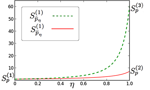
Figure 1: Behavior of $S_{\overline{p}_{\eta}}^{(1)}$ and $S_{\widehat{p}_{\eta}}^{(1)}$ for $\eta\in[0;1]$.

For each problem, the exact value of $||H^{U,V}_{S}-H^{U,V}_{p}||_{2}$ is computed for sets $U$ and $V$ of the form $\Sigma^{\leq l}$, trying to maximize $l$ according to our computing resources. It is compared to the bounds provided by Theorem 3 and Equation (1), with $\delta=0.05$ (Table 2). The optimized bound (”opt.”), refers to the case where $\sigma^{2}$ has been calculated over $U\times V$ rather than $\Sigma^{*}\times\Sigma^{*}$ (see the remark at the end of Section 3.1). Tables 3 and 4 show analog comparisons for the prefix and the factor cases with different values of $\eta$. Similar results have been obtained for all the problems of PautomaC.

Table 2: Concentration values from various bounds for $||H^{U,V}_{S}-H^{U,V}_{p}||_{2}$ for $U=V=\Sigma^{\leq l}$.

Problem number	3	4	7	15	25	29	31	38	39	40	42
$l$	8	9	8	5	5	9	7	4	6	4	7
$||H^{U,V}_{S}-H_{p}^{U,V}||_{2}$	0.0052	0.0030	0.0064	0.0037	0.0033	0.0045	0.0051	0.0058	0.0049	0.0037	0.0054
Eq. (1)	0.1910	0.0857	0.1917	0.1909	0.1935	0.1908	0.1911	0.1852	0.1925	0.1829	0.1936
Th. 3 (dim. free)	0.0669	0.0260	0.0595	0.0853	0.0761	0.0588	0.0615	0.0663	0.0692	0.0728	0.0634
Th. 3 (opt. $\boldmath{U,V}$)	0.0475	0.0228	0.0527	0.0284	0.0323	0.0472	0.0437	0.0275	0.0325	0.0243	0.0378

Table 3: Concentration values from various bounds for $||\overline{H}^{U,V}_{S}-H^{U,V}_{\overline{p},\eta}||_{2}$ (prefix case) for $U=V=\Sigma^{\leq l}$.

Problem number		3	4	7	15	25	29	31	38	39	40	42
$l$		8	9	8	5	5	9	7	4	6	4	7
$||\overline{H}^{U,V}_{S}-H_{\overline{p},\eta}^{U,V}||_{2}$		0.0067	0.0035	0.0085	0.0043	0.0041	0.0055	0.0073	0.0059	0.0061	0.0044	0.0062
Eq. (1)	$\eta=\frac{1}{2}$	0.7463	0.3326	0.7545	0.7515	0.7626	0.7250	0.7369	0.7051	0.7068	0.6753	0.7146
Th. 4 (dim. free)		0.0890	0.0339	0.0777	0.1162	0.1026	0.0770	0.0811	0.0884	0.0931	0.0983	0.0844
Th. 4 (opt. $\boldmath{U,V}$)		0.0636	0.0299	0.0697	0.0398	0.0457	0.0621	0.0577	0.0366	0.0432	0.0317	0.0498
$||\overline{H}^{U,V}_{S}-H_{\overline{p},\eta}^{U,V}||_{2}$		0.0141	0.0059	0.0217	0.0124	0.0145	0.0116	0.0182	0.0132	0.0135	0.0089	0.0127
Eq. (1)	$\eta=\small 1$	3.1011	1.3079	2.7839	3.5129	3.0283	2.9286	2.6695	2.2395	2.8524	2.5132	2.7863
Th. 4 (dim. free)		0.1784	0.0582	0.1279	0.2967	0.2261	0.1450	0.1547	0.1899	0.2230	0.2472	0.1846
Th. 4 (opt. $\boldmath{U,V}$)		0.1281	0.0518	0.1166	0.1062	0.1057	0.1175	0.1099	0.0778	0.1020	0.0761	0.1077

Table 4: Concentration values from various bounds for $||\widehat{H}^{U,V}_{S}-H^{U,V}_{\hat{p},\eta}||_{2}$ (factor case) for $U=V=\Sigma^{\leq l}$.

Problem number		3	4	7	15	25	29	31	38	39	40	42
$l$		6	7	5	4	4	6	6	4	4	4	5
$||\widehat{H}^{U,V}_{S}-H_{\widehat{p},\eta}^{U,V}||_{2}$		0.0065	0.0031	0.0071	0.0042	0.0033	0.0051	0.0072	0.0061	0.0065	0.0047	0.0060
Eq. (1)	$\eta=\frac{1}{e}$	0.9134	0.4107	0.9196	0.9466	0.9152	0.9096	0.9219	0.8765	0.8292	0.8796	0.8565
Th. 5 (dim. free)		0.0985	0.0374	0.0858	0.1292	0.1139	0.0849	0.0895	0.0979	0.1033	0.1092	0.0934
Th. 5 (opt. $\boldmath{U,V}$)		0.0601	0.0300	0.0619	0.0364	0.0412	0.0559	0.0589	0.0405	0.0356	0.0349	0.0444

We can remark that our dimension-free bounds are significantly more accurate than the one provided by Equation (1). Notice that in the prefix case, the dimension-free bound has a better behavior in the limit case $\eta=1$ than the bound from Eq. (1). This is due to the fact that in our bound, the term that bounds $||Z||_{2}$ appears in the $\frac{1}{N}$ term while it appears in the $\frac{1}{\sqrt{N}}$ term in the other one.

Implication for learning

These results show that the concentration of the empirical Hankel matrix around its mean does not highly depend on its dimension and they suggest that as far as computational resources permit it, the size of the matrices should not be artificially restricted in spectral algorithms for learning HMMs or rational stochastic languages.

To illustrate this claim, we have performed additional experiments by considering matrices with 3,000 columns and a variable number of rows, from 70 to 3,000.

For each problem and each set of rows and columns, we have computed the $r$ first right singular vectors $R$ of $H^{U,V}$ (resp. $R_{S}$ of $H_{S}^{U,V}$), where $r$ is the rank of the target, and the distance between the linear spaces spanned by $R$ and $R_{S}$. Most classical distances are based on the principal angles $\theta_{1}\geq\theta_{2}\geq\ldots\geq\theta_{r}$ between the spaces $span(R)$ and $span(R_{S})$. The largest principal angle $\theta_{1}$ is a harsh measure since, even if the two spaces coincide along the last $r-1$ principal angles, the distance between the two spaces can be large. We have considered the following measure

$$d(span(R),span(R_{S}))=1-\frac{1}{r}\sum_{i=1}^{r}\cos{\theta_{i}}$$ (3)

which is equal to 0 if the spaces coincide and 1 if they are completely orthogonal, and which takes into account all the principal angles.

The table 5 shows the sum $\sum_{i=1}^{r}\cos{\theta_{i}}$ for each problem. The table 6 displays the same information but each measure is normalised by using formula 3.

These tables show that for all problems but two, the spaces spanned by the right singular vectors are the closest for the maximal size Hankel matrix. They also show that these spaces remain quite distant for 6 problems over 11. For 4 problems, the spaces are already close to each other even for small matrices - but it can be noticed that widening the matrix do not deteriorate the results.

Table 5: Sum of the cosinus of the principal angles for each problem using matrices of dimension $|U|\times 3000$.

$|U|$	3	4	7	15	25	29	31	38	39	40	42
70	17.67	9.97	10.98	19.08	5.63	23.94	10.89	6.46	5.16	39.31	5.91
100	17.97	9.97	10.98	19.18	6.59	26.80	10.93	6.75	5.19	40.31	5.95
200	18.31	9.98	11.99	20.17	6.93	26.99	11.12	7.13	5.82	42.14	5.95
500	18.76	9.98	11.99	21.47	7.13	27.49	11.13	7.94	5.63	43.54	5.95
1000	18.82	9.98	11.99	21.53	7.82	27.88	11.16	8.38	5.60	44.94	5.95
2000	19.02	9.98	11.99	21.76	7.98	27.86	11.19	8.38	5.52	45.22	5.95
3000	19.07	9.98	11.99	21.79	7.61	27.89	11.20	8.47	5.48	45.68	5.95
rank	25	10	12	26	14	36	12	13	6	65	6

Table 6: Normalized distance between the principal angles for each problem using matrices of dimension $|U|\times 3000$.

$|U|$	3	4	7	15	25	29	31	38	39	40	42
70	0,293	0,003	0,085	0,266	0,598	0,335	0,093	0,503	0,140	0,395	0,015
100	0,281	0,003	0,085	0,262	0,529	0,256	0,089	0,481	0,135	0,380	0,008
200	0,268	0,002	0,001	0,224	0,505	0,250	0,073	0,452	0,030	0,352	0,008
500	0,250	0,002	0,001	0,174	0,491	0,236	0,072	0,389	0,062	0,330	0,008
1000	0,247	0,002	0,001	0,172	0,441	0,226	0,070	0,355	0,067	0,309	0,008
2000	0,239	0,002	0,001	0,163	0,430	0,226	0,068	0,355	0,080	0,304	0,008
3000	0,237	0,002	0,001	0,162	0,456	0,225	0,067	0,348	0,087	0,297	0,008
rank	25	10	12	26	14	36	12	13	6	65	6

5 Conclusion

We have provided dimension-free concentration inequalities for Hankel matrices in the context of spectral learning of rational stochastic languages. These bounds cover 3 cases, each one corresponding to a specific way to exploit the strings under observation, paying attention to the strings themselves, to their prefixes or to their factors. For the last two cases, we introduced parametrized variants which allow a trade-off between the rate of the concentration and the exploitation of the information contained in data.

A consequence of these results is that there is no a priori good reason, aside from computing resources limitations, to restrict the size of the Hankel matrices. This suggests an immediate future work consisting in investigating recent random techniques (Halko et al., 2011) to compute singular values decomposition on Hankel matrices in order to be able to deal with huge matrices. Then, a second aspect is to evaluate the impact of these methods on the quality of the models, including an empirical evaluation of the behavior of the standard approach and its prefix and factor extensions, along with the influence of the parameter $\eta$.

Another research direction would be to link up the prefix and factor cases to concentration bounds for sum of random tensors and to generalize the results to the case where a fixed number $\geq 1$ of factors is considered for each string.

Acknowledments

This work was supported by the French National Agency for Research (Lampada - ANR-09-EMER-007).

References

- Anandkumar et al. (2012a) Anandkumar, A., Foster, D.P., Hsu, D., Kakade, S., and Liu, Y.-K. A spectral algorithm for latent dirichlet allocation. In Proceedings of NIPS, pp. 926–934, 2012a.
- Anandkumar et al. (2012b) Anandkumar, A., Hsu, D., Huang, F., and Kakade, S. Learning mixtures of tree graphical models. In Proceedings of NIPS, pp. 1061–1069, 2012b.
- Anandkumar et al. (2012c) Anandkumar, A., Hsu, D., and Kakade, S.M. A method of moments for mixture models and hidden markov models. Proceedings of COLT - Journal of Machine Learning Research - Proceedings Track, 23:33.1–33.34, 2012c.
- Bailly (2011) Bailly, R. Méthodes spectrales pour l’inférence grammaticale probabiliste de langages stochastiques rationnels. PhD thesis, Aix-Marseille Université, 2011.
- Bailly et al. (2009) Bailly, R., Denis, F., and Ralaivola, L. Grammatical inference as a principal component analysis problem. In Proceedings of ICML, pp. 5, 2009.
- Bailly et al. (2010) Bailly, R., Habrard, A., and Denis, F. A spectral approach for probabilistic grammatical inference on trees. In Proceedings of ALT, pp. 74–88, 2010.
- Balle & Mohri (2012) Balle, B. and Mohri, M. Spectral learning of general weighted automata via constrained matrix completion. In Proceedings of NIPS, pp. 2168–2176, 2012.
- Balle et al. (2011) Balle, B., Quattoni, A., and Carreras, X. A spectral learning algorithm for finite state transducers. In Proceedings of ECML/PKDD (1), pp. 156–171, 2011.
- Balle et al. (2012) Balle, B., Quattoni, A., and Carreras, X. Local loss optimization in operator models: A new insight into spectral learning. In Proceedings of ICML, 2012.
- Balle et al. (2013) Balle, B., Carreras, X., Luque, F. M., and Quattoni, A. Spectral learning of weighted automata: A forward-backward perspective. To appear in Machine Learning, 2013.
- Cohen et al. (2012) Cohen, Shay B., Stratos, Karl, Collins, Michael, Foster, Dean P., and Ungar, Lyle H. Spectral learning of Latent-Variable PCFGs. In ACL (1), pp. 223–231. The Association for Computer Linguistics, 2012. ISBN 978-1-937284-24-4.
- Droste et al. (2009) Droste, M., Kuich, W., and Vogler, H. (eds.). Handbook of Weighted Automata. Springer, 2009.
- Halko et al. (2011) Halko, N., Martinsson, P.G., and Tropp, J.A. Finding structure with randomness: Probabilistic algorithms for constructing approximate matrix decompositions. SIAM Rev., 53(2):217–288, 2011.
- Hsu et al. (2009) Hsu, D., Kakade, S.M., and Zhang, T. A spectral algorithm for learning hidden markov models. In Proceedings of COLT, 2009.
- Hsu et al. (2011) Hsu, D., Kakade, S. M., and Zhang, T. Dimension-free tail inequalities for sums of random matrices. ArXiv e-prints, 2011.
- Kakade (2010) Kakade, S. Multivariate analysis, dimensionality reduction, and spectral methods. Lecture Notes (Matrix Concentration Derivations), 2010.
- Luque et al. (2012) Luque, F.M., Quattoni, A., Balle, B., and Carreras, X. Spectral learning for non-deterministic dependency parsing. In Proceedings of EACL, pp. 409–419, 2012.
- Parikh et al. (2011) Parikh, A.P., Song, L., and Xing, E.P. A spectral algorithm for latent tree graphical models. In Proceedings of ICML, pp. 1065–1072, 2011.
- Siddiqi et al. (2010) Siddiqi, S., Boots, B., and Gordon, G.J. Reduced-rank hidden Markov models. In Proceedings of the Thirteenth International Conference on Artificial Intelligence and Statistics (AISTATS-2010), 2010.
- Song et al. (2010) Song, L., Boots, B., Siddiqi, S.M., Gordon, G.J., and Smola, A.J. Hilbert space embeddings of hidden markov models. In Proceedings of ICML, pp. 991–998, 2010.
- Stewart (1990) Stewart, G. W. Perturbation theory for the singular value decomposition. In SVD and Signal Processing II: Algorithms, Analysis and Applications, pp. 99–109. Elsevier, 1990.
- Tropp (2012) Tropp, J.A. User-friendly tail bounds for sums of random matrices. Foundations of Computational Mathematics, 12(4):389–434, 2012.
- Verwer et al. (2012) Verwer, S., Eyraud, R., and de la Higuera, C. Results of the PAutomaC probabilistic automaton learning competition. Journal of Machine Learning Research - Proceedings Track, 21:243–248, 2012.