Higgs boson decay into two photons in an electromagnetic background field

Abstract

The amplitude for Higgs boson decay into two photons in a homogeneous and time-independent magnetic field is investigated by proper-time regularization in a gauge invariant manner and is found to be singular at large field values. The singularity is caused by the component of the charged vector boson field that is tachyonic in a strong magnetic field. Also tools for the computation of the amplitude in a more general electromagnetic background are developed.
PACS numbers 11.15.-q, 12.15.-y, 12.15.Lk, 14.70. Fm.

1 Introduction

Soon after the discovery of the 126 GeV Higgs boson [1], [2] it was pointed out by Olesen [3] (cf. also [4]) that a large magnetic field is generated by the quarks producing the Higgs boson, and that this magnetic field might influence the decay processes of the Higgs boson, and in particular the decay $H\rightarrow\gamma\gamma$ (a Higgs boson decaying to two photons).

In the present paper it is proven that this indeed is the case. The amplitude for this decay process is considered for the unrealistic case of a stationary homogeneous magnetic field $B$ by the method of Schwinger [5], further developed by Adler [6] and by Tsai and Erber [7]. It is demonstrated that the amplitude contains a term proportional to

$$\frac{eB}{M_{H}^{3}\sqrt{M_{W}^{2}-eB-\frac{1}{4}M_{H}^{2}}}$$ (1)

(with $eB>0$) for emission of photons along the field lines, with $e$ the fundamental electric charge unit, $M_{W}$ the W-boson mass and $M_{H}$ the Higgs boson mass. The amplitude is thus singular at $B=\frac{1}{e}(M_{W}^{2}-\frac{1}{4}M_{H}^{2})<B_{\rm crit}$, where $B_{\rm crit}=\frac{M_{W}^{2}}{e}$ is the critical field strength where a component of the $W$-field becomes tachyonic [8], [9]. The singularity is caused by this would-be tachyonic field component (in agreement with Olesen’s prediction [3]) and also by the fact that charged particles only propagate along the field lines, such that their loop Feynman integrals are effectively two-dimensional. The amplitude is exponentially damped for emission of photons not aligned with the magnetic field, and the denominator is modified in this case.

The amplitude of Higgs boson decay to two photons was first computed many years ago by Ellis, Gaillard and Nanopoulos [10] (see also [11]-[14]). The influence of a background field on the amplitude has not been considered before, but the pioneering paper by Vanyashin and Terentev [15] dealing with the Heisenberg-Euler effective action caused by a charged vector field makes it possible to find the behavior of the amplitude in the limit where the photon energies are close to zero, which is only possible with a Higgs boson mass also close to zero. The result described above deals with a more general situation, and the factor $\frac{1}{M_{H}^{3}}$ makes a direct comparison difficult. It turns out that the singularity of (1) can not be found from the Heisenberg-Euler effective action.

An issue relevant for the calculation is that of gauge parameter independence, where it recently was shown that the $H\rightarrow\gamma\gamma$ amplitude is the same in all $R_{\xi}$-gauges [14]. This statement can be extended to a general electromagnetic background field, using methods developed in a recent publication [16], but the proof is omitted here because of its excessive length . It is plausible that a background field does not upset the proof of gauge parameter independence since the leading singularities of propagators at short distances are independent of the background field. In general one expects gauge parameter independence of the amplitude in a regularization scheme respecting BRST invariance (this can be seen from [17], sec. 4, and also from [18]). With this justification a particular gauge (the Feynman gauge) is used throughout this paper.

The layout of the paper is as follows: In sec. 2 the standard electroweak theory is recapitulated and used to formulate an effective action at one-loop order describing Higgs boson decay to two photons in a background electromagnetic field. Formal developments in this construction are dealt with at length in app. A. It is also demonstrated in sec. 2 how the decay amplitude obtained by dimensional regularization is found from the effective action by the proper-time method, and a heuristic argument is given for (1).

Sections 3 and 4 constitute the central part of the paper. Sec. 3 contains a derivation of the decay amplitude in a general homogeneous field by the methods of [5], [6], [7], while the singular terms in a homogeneous magnetic field are extracted from the amplitude in sec. 4. App. B contains material on propagators and the associated kernels relevant for the following sections in the context of proper-time regularization. In app. C it is proven that the amplitude as well as its singular terms are invariant under gauge transformations of the radiation field. App. D. gives details on the connection to the Heisenberg-Euler effective action [15].

Finally quark contributions to the amplitude are considered in sec. 5 and found not to give rise to singularities induced by the magnetic field, while the Higgs boson self energy is shown in sec. 6 to possess a singularity similar to (1).

2 Electroweak theory and $H\rightarrow\gamma\gamma$ decay effective action

2.1 Electroweak theory

The metric is $\eta_{\mu\nu}=(+---).$

In the standard electroweak theory the scalar Lagrangian is, keeping only terms relevant for Higgs boson decay to photons, with the Higgs boson field denoted $H$, the charged Goldstone boson fields $\chi^{\pm}$ and charged vector boson fields $W^{\pm}_{\mu}$:

$${\cal L}_{\rm sc}=\frac{1}{2}(\partial_{\mu}H+\frac{g}{2}(W^{-}_{\mu}\chi^{+}+W^{+}_{\mu}\chi^{-}))^{2}+(\chi^{+}\stackrel{{\scriptstyle\leftarrow}}{{D}}^{\mu}-\frac{g}{2}W^{+\mu}H)(D_{\mu}\chi^{-}-\frac{g}{2}W^{-}_{\mu}H)$$

$$-\frac{1}{2}\mu^{2}(2\chi^{+}\chi^{-}+H^{2})-\frac{\lambda}{4}(2\chi^{+}\chi^{-}+H^{2})^{2}$$ (2)

with the coupling constants $g$. By the Higgs mechanism one makes the replacement $H\rightarrow v+H,v=\sqrt{\frac{-\mu^{2}}{\lambda}}$, and $W^{\pm}$ get the mass $M_{W}=\frac{gv}{2}$, while the Higgs boson mass is $M_{H}=\sqrt{2\lambda}v$. The covariant derivatives are:

$$D_{\mu}=\partial_{\mu}-ieA_{\mu},\stackrel{{\scriptstyle\leftarrow}}{{D}}_{\mu}=\stackrel{{\scriptstyle\leftarrow}}{{\partial}}_{\mu}+ieA_{\mu}$$ (3)

with $e=g\sin\theta_{W}$ the elementary charge unit, where $\theta_{W}$ is the Weinberg angle, and with $A_{\mu}$ the electromagnetic field.

In order to describe radiation processes one splits the electromagnetic field $A_{\mu}$:

$$A_{\mu}\rightarrow A_{\mu}+{\cal A}_{\mu}$$ (4)

with $A_{\mu}$ a background field, and ${\cal A}_{\mu}$ the radiation field, which fulfils the wave equation and has two independent transverse polarizations. The interaction between radiation and $W$-bosons is described by the action:

$$-\int d^{4}xW^{+\nu}{\cal H}_{\nu\mu}W^{-\mu}$$

with ${\cal H}$ given by:

$${\cal H}_{\nu\mu}=-2ie{\cal F}_{\mu\nu}+2ie\eta_{\mu\nu}{\cal A}^{\lambda}D_{\lambda}+ie(\stackrel{{\scriptstyle\leftarrow}}{{D}}_{\nu}{\cal A}_{\mu}-{\cal A}_{\nu}D_{\mu})-e^{2}({\cal A}_{\mu}{\cal A}_{\nu}-\eta_{\mu\nu}{\cal A}^{\lambda}{\cal A}_{\lambda})$$

$$={\cal H}^{(1)}_{\nu\mu}+{\cal H}^{[2]}_{\nu\mu}$$ (5)

where the superscript denotes the order in $e$ and where we introduced the radiation field strength:

$${\cal F}_{\mu\nu}=\partial_{\mu}{\cal A}_{\nu}-\partial_{\nu}{\cal A}_{\mu}.$$ (6)

The following relations followis from (5) and the on-shell properties of the radiation field ${\cal A}_{\mu}$:

$$D^{\nu}{\cal H}^{(1)}_{\nu\mu}=-ie{\cal A}^{\nu}(\eta_{\nu\mu}D^{2}+D_{\nu}D_{\mu}-2D_{\mu}D_{\nu}),$$

$${\cal H}^{(1)}_{\nu\mu}\stackrel{{\scriptstyle\leftarrow}}{{D}}^{\mu}=ie(\eta_{\nu\mu}\stackrel{{\scriptstyle\leftarrow}}{{D}}^{2}+\stackrel{{\scriptstyle\leftarrow}}{{D}}_{\nu}\stackrel{{\scriptstyle\leftarrow}}{{D}}_{\mu}-2\stackrel{{\scriptstyle\leftarrow}}{{D}}_{\mu}\stackrel{{\scriptstyle\leftarrow}}{{D}}_{\nu}){\cal A}^{\mu}$$ (7)

which should be understood as relations between differential operators.

The gauge of $W^{\pm}$ is fixed by:

$$\mathcal{L}_{\rm gf}=-(W^{+,\mu}\stackrel{{\scriptstyle\leftarrow}}{{D}}_{\mu}+\frac{gv}{2}\chi^{+})(D_{\nu}W^{-,\nu}+\frac{gv}{2}\chi^{-})$$ (8)

(the $R_{\xi}$ Feynman gauge). By (8) a Goldstone boson mass squared $M_{W}^{2}$ is generated. The Faddeev-Popov ghost Lagrangian is:

$${\cal L}_{\rm FP}=-\bar{c}^{+}(c^{+}\stackrel{{\scriptstyle\leftarrow}}{{D}}^{2}+ie({\cal A}^{\mu}c^{+})\stackrel{{\scriptstyle\leftarrow}}{{D}}_{\mu}+\frac{g^{2}v}{4}Hc^{+})-\bar{c}^{-}(D^{2}c^{-}-ieD_{\mu}({\cal A}^{\mu}c^{-})+\frac{g^{2}v}{4}Hc^{-})$$ (9)

so the ghost mass is equal to the Goldstone boson mass.

2.2 Proper-time representation of the scalar and vector propagators in a general background

The scalar propagator $G_{\rm sc}(x,x^{\prime})$ corresponding to the mass $M_{W}^{2}$ is given by:

$$G_{{\rm sc}}(x,x^{\prime})=\int_{0}^{\infty}d\tau h_{{\rm sc}}(x,x^{\prime};\tau)$$ (10)

with $D^{2}=\eta^{\mu\nu}D_{\mu}D_{\nu}$ and with $\tau$ the proper time variable [5], [19], and:

$$(D^{2}+M_{W}^{2})G_{{\rm sc}}(x,x^{\prime})=G_{{\rm sc}}(x,x^{\prime})(\stackrel{{\scriptstyle\leftarrow}}{{D^{\prime}}}^{2}+M_{W}^{2})=-i\delta(x-x^{\prime})$$ (11)

where a primed derivative refers to $x^{\prime}$ and where the scalar kernel $h_{{\rm sc}}(x,x^{\prime};\tau)$ is defined by:

$$(i\frac{\partial}{\partial\tau}-(D^{2}+M_{W}^{2}))h_{{\rm sc}}(x,x^{\prime};\tau)=0,\ h_{{\rm sc}}(x,y;0)=\delta(x-x^{\prime}).$$ (12)

The vector propagator $G_{{\rm vec},\mu\nu}(x,x^{\prime})$ is similarly defined by:

$$(D^{2}+M_{W}^{2})G_{{\rm vec},\mu\nu}(x,x^{\prime})-2ieF_{\mu\lambda}(x)G_{{\rm vec},}^{\lambda}\hskip 0.28453pt{}_{\nu}(x,x^{\prime})$$

$$=G_{{\rm vec},\mu\nu}(x,x^{\prime})(\stackrel{{\scriptstyle\leftarrow}}{{D^{\prime}}}^{2}+M_{W}^{2})-G_{{\rm vec},\mu}^{\lambda}(x,x^{\prime})2ieF_{\lambda\nu}(x^{\prime})$$

$$=i\eta_{\mu\nu}\delta(x,x^{\prime})$$ (13)

where $F_{\mu\nu}=\partial_{\mu}A_{\nu}-\partial_{\nu}A_{\mu}$ is the background field strength. The solution of (13) is:

$$G_{{\rm vec},\mu\nu}(x,x^{\prime})=\int_{0}^{\infty}d\tau h_{{\rm vec},\mu\nu}(x,x^{\prime};\tau)$$ (14)

with:

$$(i\frac{\partial}{\partial\tau}-(D^{2}+M_{W}^{2}))h_{{\rm vec},\mu\nu}(x,x^{\prime};\tau)+2ieF_{\mu}\hskip 0.28453pt^{\lambda}h_{{\rm vec},\lambda\nu}(x,x^{\prime};\tau)=0,$$

$$h_{{\rm vec},\mu\nu}(x,x^{\prime};0)=-\eta_{\mu\nu}\delta(x-x^{\prime})$$ (15)

defining the vector kernel corresponding to the scalar kernel defined by (12). The integration path in (10) and (14) can be deformed such that it runs below the real axis or along the negative imaginary axis in the complex $\tau$-plane, provided no field components are tachyonic.

The following Ward identities hold for the kernels:

$$D^{\mu}h_{{\rm vec},\mu\nu}(x,x^{\prime};\tau)=h_{{\rm sc}}(x,x^{\prime};\tau)\stackrel{{\scriptstyle\leftarrow}}{{D}}_{\nu},$$

$$h_{{\rm vec},\mu\nu}(x,x^{\prime};\tau)\stackrel{{\scriptstyle\leftarrow}}{{D}}^{\nu}=D_{\mu}h_{{\rm sc}}(x,x^{\prime};\tau)$$ (16)

since both sides of the two equations obey the same first-order differential equations in $\tau$ with the same boundary conditions; here was also used:

$$D^{\nu}D^{2}-D^{2}D^{\nu}=-2ieF^{\nu\lambda}D_{\lambda}.$$ (17)

following from the defintion of the covariant derivative and the fact that the background field is a solution of the Maxwell equations. From (16) follows the Ward identities of propagators:

$$D^{\mu}G_{{\rm vec},\mu\nu}(x,x^{\prime})=G_{{\rm sc}}(x,x^{\prime})\stackrel{{\scriptstyle\leftarrow}}{{D}}_{\nu},$$

$$G_{{\rm vec},\mu\nu}(x,x^{\prime})\stackrel{{\scriptstyle\leftarrow}}{{D}}_{\nu}=D_{\mu}G_{{\rm sc}}(x,x^{\prime}).$$ (18)

2.3 $H\rightarrow\gamma\gamma$ decay effective action

A background Higgs boson field $H(x)$ is used here which is on-shell, i.e.

$$(\partial^{2}+2\lambda v^{2})H(x)=0.$$ (19)

The effective action terms determining the $H$ decay amplitude at one-loop order in terms of the propagators described previously are determined from (2). One term of the effective action is:

$$S_{I}=-2i\lambda e^{2}v\int d^{4}x\int d^{4}yH(x)G_{{\rm sc}}(x,y){\cal A}^{\nu}(y){\cal A}_{\nu}(y)G_{\rm{sc}}(y,x)$$

$$-8\lambda e^{2}v\int d^{4}x\int d^{4}y\int d^{4}zH(x)G_{{\rm sc}}(x,y){\cal A}^{\nu}(y)D_{\nu}G_{{\rm sc}}(y,z){\cal A}^{\lambda}(z)D_{\lambda}G_{{\rm sc}}(z,x)$$ (20)

which is a seagull term and a derivative coupling term in the way familiar from scalar quantum electrodynamics, with a Higgs boson insertion in one propagator. The remaining effective action terms are (101)-(107) listed in app. A. Remarkably, they can be reduced to a structure similar to (20), with both scalar and vector internal propagators, and in the latter case also with magnetic moment couplings. The reduction takes place by means of (7) and (18).

In (101) one isolates the following three expressions by insertion of (5):

$$S_{II}^{\prime}=-ie^{2}gM_{W}\int d^{4}yH(x)G_{{\rm vec}}\hskip 0.28453pt^{\mu\lambda}(x,y){\cal A}^{\nu}(y){\cal A}_{\nu}(y)G_{{\rm vec},\lambda\mu}(y,x)$$

$$+4e^{2}gM_{W}\int d^{4}x\int d^{4}y\int d^{4}zH(x)G_{{\rm vec},\mu}\hskip 0.28453pt^{\rho}(x,y)$$

$${\cal A}^{\nu}(y)D_{\nu}G_{{\rm vec},\rho}\hskip 0.28453pt^{\sigma}(y,z){\cal A}^{\lambda}(z)D_{\lambda}G_{{\rm vec},\sigma}\hskip 0.28453pt^{\mu}(z,x),$$ (21)

which obviously is similar to (20),

$$S_{III}^{\prime}=4e^{2}gM_{W}\int d^{4}x\int d^{4}y\int d^{4}zH(x)$$

$$G_{{\rm vec},\mu\lambda}(x,y){\cal F}^{\lambda\rho}(y)G_{{\rm vec},\rho\sigma}(y,z){\cal F}^{\sigma\omega}(z)G_{{\rm vec},\omega}\hskip 0.28453pt^{\mu}(z,x),$$ (22)

with magnetic moment couplings, and:

$$S_{IV}^{\prime}=-4e^{2}gM_{W}\int d^{4}x\int d^{4}y\int d^{4}zH(x)$$

$$(G_{{\rm vec},\mu\rho}(x,y){\cal F}^{\rho\sigma}(y)G_{{\rm vec},\sigma\omega}(y,z){\cal A}^{\lambda}(z)D_{\lambda}G_{{\rm vec},}\hskip 0.28453pt^{\omega\mu}(z,x)$$

$$+G_{{\rm vec},\mu\rho}(x,y){\cal A}^{\nu}(x)D_{\nu}G_{{\rm vec},}\hskip 0.28453pt^{\rho}\hskip 0.28453pt{}_{\omega}(y,z){\cal F}^{\omega\epsilon}(z)G_{{\rm vec},\epsilon}\hskip 0.28453pt^{\mu}(z,x)).$$ (23)

with a derivative coupling at one vertex and a magnetic moment coupling at the other vertex. Adding the rest of (101) to (102)-(107) one obtains as shown in app. A:

$$S_{V}^{\prime}=ie^{2}gM_{W}\int d^{4}x\int d^{4}yH(x)G_{{\rm sc}}(x,y){\cal A}^{\nu}{\cal A}_{\nu}(y)G_{{\rm sc}}(y,x)$$

$$+4e^{2}gM_{W}\int d^{4}x\int d^{4}y\int d^{4}zH(x)G_{{\rm sc}}(x,y){\cal A}^{\nu}(y)D_{\nu}G_{{\rm sc}}(y,z){\cal A}^{\lambda}(z)D_{\lambda}G_{{\rm sc}}(z,x)$$ (24)

with the same structure as (20) or (21).

A Feynman diagram representation of $S_{I}$ and $S_{II}^{\prime}-S_{V}^{\prime}$ is given in Figure 1.

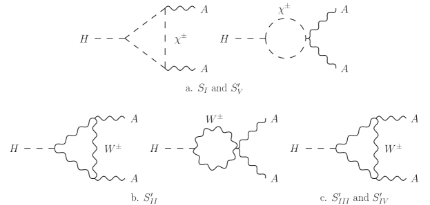
Figure 1: Feynman diagram representation of the effective action in its final form.

2.4 $H\rightarrow\gamma\gamma$ decay amplitude in a vanishing external field

From (20) and (21)-(24) the amplitude of the decay of a Higgs boson to two photons is found. Here and elsewhere in the paper the photon momenta and polarization vectors are denoted $k,\varepsilon_{\mu}(k)$ and $q,\varepsilon_{\nu}(q)$, with $k\cdot\epsilon(k)=q\cdot\epsilon(q)=0$. The evaluation is carried out by means of (10), (12), (14) and (15).

In the limit where the background field vanishes the contribution from (21) to the amplitude is in the proper-time representation:

$$-8ie^{2}gM_{W}\varepsilon^{\mu}(k)\varepsilon_{\mu}(q)\int_{0}^{\infty}\tau d\tau\int_{0}^{1}d\alpha\int\frac{d^{4}r}{(2\pi)^{4}}e^{i\tau((1-\alpha)r^{2}+\alpha(p-r)^{2}-M_{W}^{2})}$$

$$+16e^{2}gM_{W}\varepsilon^{\mu}(k)\varepsilon^{\nu}(q)\int_{0}^{\infty}\tau^{2}d\tau e^{-i\tau M_{W}^{2}}\int_{0}^{1}d\alpha d\beta d\gamma\delta(1-\alpha-\beta-\gamma)$$

$$\int\frac{d^{4}r}{(2\pi)^{4}}\bigg{(}r_{\mu}(r+k)_{\nu}e^{i\tau(\alpha r^{2}+\beta(k+r)^{2}+\gamma(k+q+r)^{2})}+r_{\nu}(r+q)_{\mu}e^{i\tau(\alpha r^{2}+\beta(q+r)^{2}+\gamma(k+q+r)^{2})}\bigg{)}$$

(25)

where the integrations of the proper time $\tau$ are carried out after the integrations of the momentum variable $r$; the momentum integrations are convergent at nonvanishing values of the proper time. Here a factor $(2\pi)^{4}\delta(p-k-q)$ is suppressed, with $p$ the Higgs boson momentum. After some manipulations one gets from (25), using the mass-shell conditions as well as symmetric integration in four dimensions:

$$-8ie^{2}gM_{W}\varepsilon^{\mu}(k)\varepsilon_{\mu}(q)\int_{0}^{\infty}\tau d\tau\int_{0}^{1}d\alpha\int\frac{d^{4}r}{(2\pi)^{4}}e^{i\tau(r^{2}+\alpha(1-\alpha)M_{H}^{2}-M_{W}^{2})}$$

$$+16e^{2}gM_{W}\varepsilon^{\mu}(k)\varepsilon_{\mu}(q)\int_{0}^{\infty}\tau^{2}d\tau e^{-i\tau M_{W}^{2}}\int_{0}^{1}d\alpha\int_{0}^{1-\alpha}d\gamma\int\frac{d^{4}r}{(2\pi)^{4}}e^{i\tau(r^{2}+\alpha\gamma M_{H}^{2})}(\frac{1}{2}r^{2}-\alpha\gamma M_{H}^{2})$$

$$+32e^{2}gM_{W}\varepsilon^{\mu}(k)\varepsilon^{\nu}(q)(q\cdot k\eta_{\mu\nu}-q_{\mu}k_{\nu})\int_{0}^{\infty}\tau^{2}d\tau e^{-i\tau M_{W}^{2}}\int_{0}^{1}d\alpha\int_{0}^{1-\alpha}d\gamma\alpha\gamma\int\frac{d^{4}r}{(2\pi)^{4}}e^{i\tau(r^{2}+\alpha\gamma M_{H}^{2})}.$$

(26)

In (26) one uses:

$$\int\frac{d^{4}r}{(2\pi)^{4}}e^{i\tau r^{2}}=-\frac{i}{16\pi^{2}\tau^{2}}$$ (27)

and also:

$$\int_{0}^{\infty}\tau^{2}d\tau e^{-i\tau M_{W}^{2}}\int_{0}^{1}d\alpha\int_{0}^{1-\alpha}d\gamma\int\frac{d^{4}r}{(2\pi)^{4}}e^{i\tau(r^{2}+\alpha\gamma M_{H}^{2})}(\frac{1}{2}r^{2}-\alpha\gamma M_{H}^{2})$$

$$=\frac{1}{2}\frac{1}{16\pi^{2}}\int_{0}^{\infty}\frac{d\tau}{\tau}e^{-i\tau M_{W}^{2}}\int_{0}^{1}d\alpha e^{i\alpha(1-\alpha)\tau M_{H}^{2}}.$$ (28)

Evaluating (26) by (27) and (28) one finds that the first two terms cancel out, and (26) reduces to:

$$-\frac{2e^{2}gM_{W}}{\pi^{2}}\varepsilon^{\mu}(k)\varepsilon^{\nu}(q)(q\cdot k\eta_{\mu\nu}-q_{\mu}k_{\nu})\int_{0}^{1}d\alpha\int_{0}^{1-\alpha}d\gamma\frac{\alpha\gamma}{M_{W}^{2}-\alpha\gamma M_{H}^{2}}$$

$$=\frac{e^{2}gM_{W}}{\pi^{2}M_{H}^{2}}\varepsilon^{\mu}(k)\varepsilon^{\nu}(q)(q\cdot k\eta_{\mu\nu}-q_{\mu}k_{\nu})(1-\frac{4M_{W}^{2}}{M_{H}^{2}}\arcsin^{2}(\frac{M_{H}}{2M_{W}})).$$ (29)

The total contribution to the amplitude from (20), (21) and (24) is found from (29) by the substitution:

$$4e^{2}gM_{W}\rightarrow 2\lambda e^{2}v+3e^{2}gM_{W}.$$ (30)

(22) in a vanishing external field contributes to the decay amplitude:

$$-4e^{2}gM_{W}(k^{\mu}\varepsilon^{\nu}(k)-k^{\nu}\varepsilon^{\mu}(k))(q_{\mu}\varepsilon_{\nu}(q)-q_{\nu}\varepsilon_{\mu}(q))$$

$$\int_{0}^{\infty}\tau^{2}d\tau e^{-i\tau M_{W}^{2}}\int_{0}^{1}d\alpha d\beta d\gamma\delta(1-\alpha-\beta-\gamma)$$

$$\int\frac{d^{4}r}{(2\pi)^{4}}\bigg{(}e^{i\tau(\alpha r^{2}+\beta(k+r)^{2}+\gamma(k+q+r)^{2})}+e^{i\tau(\alpha r^{2}+\beta(q+r)^{2}+\gamma(k+q+r)^{2})}\bigg{)}$$

$$=\frac{2e^{2}gM_{W}}{\pi^{2}M_{H}^{2}}\varepsilon^{\mu}(k)\varepsilon^{\nu}(q)(q\cdot k\eta_{\mu\nu}-q_{\mu}k_{\nu})\arcsin^{2}(\frac{M_{H}}{2M_{W}}).$$ (31)

(23) is zero in a vanishing external field.

The decay amplitude with vanishing external field is the sum of (29) (with the substitution (30)) and (31):

$$\frac{e^{2}}{4\pi^{2}v}\varepsilon^{\mu}(k)\varepsilon^{\nu}(q)(q\cdot k\eta_{\mu\nu}-q_{\mu}k_{\nu})$$

$$((1+\frac{6M_{W}^{2}}{M_{H}^{2}})(1-\frac{4M_{W}^{2}}{M_{H}^{2}}\arcsin^{2}(\frac{M_{H}}{2M_{W}}))+\frac{16M_{W}^{2}}{M_{H}^{2}}\arcsin^{2}(\frac{M_{H}}{2M_{W}}))$$ (32)

which is the standard decay amplitude [10]-[14]. It is perhaps an interesting point that this result has been obtained by proper-time regularization instead of dimensional regularization; symmetrical integration in momentum space has been carried out in four dimensions and this is possible because momentum integrals are finite at nonvanishing values of the proper time $\tau$.

Carrying for the sake of argument the integral in (29) out in two space-time dimensions one gets, disregarding the dimensional mismatch, the result:

$$-\frac{8e^{2}gM_{W}}{\pi}\int_{0}^{1}d\alpha\int_{0}^{1-\alpha}d\gamma\frac{\alpha\gamma}{(M_{W}^{2}-\alpha\gamma M_{H}^{2})^{2}}$$

$$=-\frac{8e^{2}gM_{W}}{\pi M_{H}^{4}}(\frac{M_{H}}{\sqrt{M_{W}^{2}-\frac{1}{4}M_{H}^{2}}}\arcsin(\frac{M_{H}}{2M_{W}})-2\arcsin^{2}(\frac{M_{H}}{2M_{W}}))$$ (33)

This is singular at $\frac{M_{H}}{M_{W}}=2$; the singularity arises from $\alpha\simeq\gamma\simeq\frac{1}{2}$ where the denominator of the integrand is very small at this value of the mass ratio. This argument gives a heuristic indication of the way in which the square-root singularity of (1) arises, since the quasi-tachyonic field component decreases the vector boson mass according to:

$$M_{W}^{2}\rightarrow M_{W}^{2}-eB.$$ (34)

The complete determination of the singularity takes place in sec. 4.

3 $H\rightarrow\gamma\gamma$ decay amplitude in a non-vanishing homogeneous field

The $H\rightarrow\gamma\gamma$ amplitude in a non-vanishing homogeneous electromagnetic field is found from (20)-(24) by the method of Schwinger [5],[6], [7]. Details on formal tools are relegated to App.B.

The contribution from the first term of (20) to the decay amplitude is by (136):

$$-4i\lambda e^{2}v\varepsilon^{\mu}(k)\varepsilon_{\mu}(q)\int d^{4}xe^{ipx}\int_{0}^{\infty}\tau d\tau e^{-i\tau M_{W}^{2}}\int_{0}^{1}d\alpha<x\mid e^{i(1-\alpha)\tau\Pi^{2}}e^{-i(k+q)X}e^{i\alpha\tau\Pi^{2}}\mid x>$$

$$=-4i\lambda e^{2}v\varepsilon^{\mu}(k)\varepsilon_{\mu}(q)\int d^{4}xe^{ipx}\int_{0}^{\infty}\tau d\tau e^{-i\tau M_{W}^{2}}\int_{0}^{1}d\alpha<x,\tau\mid e^{-i(k+q)X(\alpha\tau)}\mid x,0>.$$ (35)

Here one uses (140), as well as the eigenvalue equation (128), to get the following value of (35) with a factor $(2\pi)^{4}\delta(p-k-q)$ suppressed (cf. [7]):

$$-4i\lambda e^{2}v\varepsilon^{\mu}(k)\varepsilon_{\mu}(q)\int_{0}^{\infty}\tau d\tau e^{-i\tau M_{W}^{2}}<x,\tau\mid x,0>\int_{0}^{1}d\alpha e^{\delta_{1}(\alpha,k+q)}.$$ (36)

Next the contribution of the second term of (20) to the decay amplitude is evaluated. It has the proper-time representation:

$$8\lambda e^{2}v\varepsilon^{\mu}(k)\varepsilon^{\nu}(q)\int d^{4}xe^{ipx}\int_{0}^{\infty}\tau^{2}d\tau e^{-i\tau M_{W}^{2}}\int_{0}^{1}d\alpha d\beta d\gamma\delta(1-\alpha-\beta-\gamma)$$

$$(<x\mid e^{i\alpha\tau\Pi^{2}}e^{-ik\cdot X}\Pi_{\mu}e^{i\beta\tau\Pi^{2}}e^{-iq\cdot X}\Pi_{\nu}e^{i\gamma\tau\Pi^{2}}\mid x>+(\mu\leftrightarrow\nu,k\leftrightarrow q))$$

$$=8\lambda e^{2}v\varepsilon^{\mu}(k)\varepsilon^{\nu}(q)\int d^{4}xe^{ipx}\int_{0}^{\infty}\tau^{2}d\tau e^{-i\tau M_{W}^{2}}\int_{0}^{1}d\alpha d\beta d\gamma\delta(1-\alpha-\beta-\gamma)$$

$$(<x,\tau\mid\Pi_{\mu}((1-\alpha)\tau)e^{-ik\cdot X((1-\alpha)\tau}e^{-iq\cdot X(\gamma\tau)}\Pi_{\nu}(\gamma\tau)\mid x,0>+(\mu\leftrightarrow\nu,k\leftrightarrow q))$$ (37)

by (133), and using here (142) and (146) as well as the procedure used above to obtain (36) one finds:

$$8\lambda e^{2}v\varepsilon^{\mu}(k)\varepsilon^{\nu}(q)\int d^{4}xe^{ipx}\int_{0}^{\infty}\tau^{2}d\tau e^{-i\tau M_{W}^{2}}\int_{0}^{1}d\alpha d\beta d\gamma\delta(1-\alpha-\beta-\gamma)$$

$$(e^{\delta_{2}(k,q)}<x,\tau\mid\Pi_{\mu}((1-\alpha)\tau)e^{-iQ\cdot X(\tau)}e^{-i(k+q-Q)\cdot X(0)}\Pi_{\nu}(\gamma\tau)\mid x,0>+(\mu\leftrightarrow\nu,k\leftrightarrow q))$$

$$=8\lambda e^{2}v\varepsilon^{\mu}(k)\varepsilon^{\nu}(q)(2\pi)^{4}\delta(p-k-q)\int_{0}^{\infty}\tau^{2}d\tau e^{-i\tau M_{W}^{2}}\int_{0}^{1}d\alpha d\beta d\gamma\delta(1-\alpha-\beta-\gamma)$$

$$(e^{\delta_{2}(k,q)}<x,\tau\mid(\Pi((1-\alpha)\tau)-e^{2\alpha\tau e{\bf F}}Q)_{\mu}(\Pi(\gamma\tau)+(e^{-2\gamma\tau e{\bf F}}(k+q-Q))_{\nu}\mid x,0>$$

$$+(\mu\leftrightarrow\nu,k\leftrightarrow q))$$ (38)

and in the last step (133) was used again.

The evaluation of (38) is carried out by (133) and (135). Only terms with two or no $\Pi$ operators give a nonvanishing contribution. With no $\Pi$ operators one gets the following contribution from (38):

$$-8\lambda e^{2}v\varepsilon^{\mu}(k)\varepsilon^{\nu}(q)\int_{0}^{\infty}\tau^{2}d\tau e^{-i\tau M_{W}^{2}}<x,\tau\mid x,0>\int_{0}^{1}d\alpha d\beta d\gamma\delta(1-\alpha-\beta-\gamma)$$

$$(e^{\delta_{2}(k,q)}(e^{2\alpha\tau e{\bf F}}Q)_{\mu}(e^{-2\gamma\tau e{\bf F}}(k+q-Q))_{\nu}+(\mu\leftrightarrow\nu,k\leftrightarrow q)).$$ (39)

The term of (38) with two $\Pi$ operators contributes:

$$8i\lambda e^{2}v\varepsilon^{\mu}(k)\varepsilon^{\nu}(q)\int_{0}^{\infty}\tau^{2}d\tau e^{-i\tau M_{W}^{2}}<x,\tau\mid x,0>\int_{0}^{1}d\alpha d\beta d\gamma\delta(1-\alpha-\beta-\gamma)$$

$$(e^{\delta_{2}(k,q)}(e^{-2\beta\tau e{\bf F}}{\bf D}^{-1}(\tau))_{\mu\nu}+(\mu\leftrightarrow\nu,k\leftrightarrow q)).$$ (40)

In both (39) and (40) a factor $(2\pi)^{4}\delta(p-k-q)$ was left out. The sum of (36), (39) and (40) is invariant under gauge transformations of the polarization vectors. This follows from the general proof in (179) (app. C) but can be proven directly also.

(36) and (40) are both ultraviolet divergent and can be rearranged in two convergent expressions:

$$8i\lambda e^{2}v\varepsilon^{\mu}(k)\varepsilon^{\nu}(q)\int_{0}^{\infty}\tau^{2}d\tau e^{-i\tau M_{W}^{2}}<x,\tau\mid x,0>\int_{0}^{1}d\alpha d\beta d\gamma\delta(1-\alpha-\beta-\gamma)$$

$$(e^{\delta_{2}(k,q)}(e^{-2\beta\tau e{\bf F}}{\bf D}^{-1}(\tau)-\frac{1}{2\tau}{\bf 1})_{\mu\nu}+(\mu\leftrightarrow\nu,k\leftrightarrow q))$$ (41)

and:

$$4i\lambda e^{2}v\varepsilon^{\mu}(k)\varepsilon_{\mu}(q)\int_{0}^{\infty}\tau d\tau e^{-i\tau M_{W}^{2}}<x,\tau\mid x,0>\int_{0}^{1}d\alpha d\beta d\gamma\delta(1-\alpha-\beta-\gamma)$$

$$((e^{\delta_{2}(k,q)}-e^{\delta_{2}(k,q)}\mid_{\gamma=1-\alpha})+(k\leftrightarrow q)).$$ (42)

The contribution of (21) to the amplitude is:

$$-2ie^{2}gM_{W}\varepsilon^{\mu}(k)\varepsilon_{\mu}(q)\int d^{4}xe^{ipx}\int_{0}^{\infty}\tau d\tau e^{-i\tau M_{W}^{2}}{\rm tr}(e^{-2\tau e{\bf F}})$$

$$\int_{0}^{1}d\alpha<x\mid e^{i(1-\alpha)\tau\Pi^{2}}e^{i(k+q)X}e^{i\alpha\tau\Pi^{2}}\mid x>$$

$$+4e^{2}gM_{W}\varepsilon^{\mu}(k)\varepsilon^{\nu}(q)\int d^{4}xe^{ipx}\int_{0}^{\infty}\tau^{2}d\tau e^{-i\tau M_{W}^{2}}\int_{0}^{1}d\alpha d\beta d\gamma\delta(1-\alpha-\beta-\gamma)$$

$${\rm tr}(e^{-2\tau e{\bf F}})(<x\mid e^{i\alpha\tau\Pi^{2}}\Pi_{\mu}e^{ik\cdot X}e^{i\beta\tau\Pi^{2}}\Pi_{\nu}e^{i\gamma\tau\Pi^{2}}\mid x>+(\mu\leftrightarrow\nu,k\leftrightarrow q))$$ (43)

and is thus determined from (39), (41) and (42) by the substitution $8\lambda e^{2}v\rightarrow 4e^{2}gM_{W}$ and insertion of a factor ${\rm tr}(e^{-2\tau e{\bf F}})$ in the integral. Also from (24) one gets three terms similar to (39), (41) and (42) by the substitution $8\lambda e^{2}v\rightarrow-4e^{2}gM_{W}.$

For the considerations on a pure magnetic field in the following section it is convenient to isolate in the contribution to the amplitude from (43) the following three terms:

$$-4e^{2}gM_{W}\varepsilon^{\mu}(k)\varepsilon^{\nu}(q)\int_{0}^{\infty}\tau^{2}d\tau e^{-i\tau M_{W}^{2}}({\rm tr}(e^{-2\tau e{\bf F}})-4)<x,\tau\mid x,0>\delta(1-\alpha-\beta-\gamma)$$

$$(e^{\delta_{2}(k,q)}(e^{2\alpha\tau e{\bf F}}Q)_{\mu}(e^{-2\gamma\tau e{\bf F}}(k+q-Q))_{\nu}+(\mu\leftrightarrow\nu,k\leftrightarrow q))$$ (44)

and also:

$$4ie^{2}gM_{W}\varepsilon^{\mu}(k)\varepsilon^{\nu}(q)\int_{0}^{\infty}\tau^{2}d\tau e^{-i\tau M_{W}^{2}}({\rm tr}(e^{-2\tau e{\bf F}})-4)<x,\tau\mid x,0>\int_{0}^{1}d\alpha d\beta d\gamma\delta(1-\alpha-\beta-\gamma)$$

$$(e^{\delta_{2}(k,q)}(e^{-2\beta\tau e{\bf F}}{\bf D}^{-1}(\tau)-\frac{1}{2\tau}{\bf 1})_{\mu\nu}+(\mu\leftrightarrow\nu,k\leftrightarrow q))$$ (45)

and:

$$2ie^{2}gM_{W}\varepsilon^{\mu}(k)\varepsilon_{\mu}(q)\int_{0}^{\infty}\tau d\tau e^{-i\tau M_{W}^{2}}({\rm tr}(e^{-2\tau e{\bf F}})-4)<x,\tau\mid x,0>\int_{0}^{1}d\alpha d\beta d\gamma\delta(1-\alpha-\beta-\gamma)$$

$$((e^{\delta_{2}(k,q)}-e^{\delta_{2}(k,q)}\mid_{\gamma=1-\alpha})+(k\leftrightarrow q))$$ (46)

and to further isolate in (44) and (46):

$$-4e^{2}gM_{W}\varepsilon^{\mu}(k)\varepsilon^{\nu}(q)\int_{0}^{\infty}\tau^{2}d\tau e^{-i\tau M_{W}^{2}}({\rm tr}(e^{-2\tau e{\bf F}})-4)<x,\tau\mid x,0>\int_{0}^{1}d\alpha d\beta d\gamma\alpha\gamma\delta(1-\alpha-\beta-\gamma)$$

$$(e^{\delta_{2}(k,q)}+e^{\delta_{2}(q,k)})(q_{\mu}k_{\nu}-\eta_{\mu\nu}q\cdot k).$$ (47)

Here was used:

$$\int_{0}^{1}d\alpha d\beta d\gamma\delta(1-\alpha-\beta-\gamma)(e^{\delta_{2}(k,q)}-e^{\delta_{2}(k,q)}\mid_{\gamma=1-\alpha})$$

$$=-\int_{0}^{1}d\alpha d\beta d\gamma\delta(1-\alpha-\beta-\gamma)\frac{1}{2}(\alpha\frac{\partial}{\partial\alpha}+\gamma\frac{\partial}{\partial\gamma})e^{\delta_{2}(k,q)}$$ (48)

and also (145). The remaining amplitude terms from (21) and (24) are obtained from (39), (41) and (42) by the substitution $2\lambda e^{2}v\rightarrow 3e^{2}gM_{W}$.

From (22) one gets:

$$4e^{2}gM_{W}\varepsilon^{\mu}(k)\varepsilon^{\nu}(q)\int d^{4}xe^{ipx}\int_{0}^{\infty}\tau^{2}d\tau e^{-i\tau M_{W}^{2}}\int_{0}^{1}d\alpha d\beta d\gamma\delta(1-\alpha-\beta-\gamma)$$

$$\bigg{(}(e^{-2(\alpha+\gamma)\tau e{\bf F}})_{\epsilon\rho}(\delta^{\rho}\hskip 0.28453pt_{\mu}k^{\sigma}-\delta^{\sigma}\hskip 0.28453pt_{\mu}k^{\rho})(e^{-2\beta\tau e{\bf F}})_{\sigma\omega}(\delta^{\omega}\hskip 0.28453pt_{\nu}q^{\epsilon}-\delta^{\epsilon}\hskip 0.28453pt_{\nu}q^{\omega})$$

$$<x\mid e^{i\alpha\tau\Pi^{2}}e^{-ik\cdot X}e^{i\beta\tau\Pi^{2}}e^{-iq\cdot X}\ e^{i\gamma\tau\Pi^{2}}\mid x>+(\mu\leftrightarrow\nu,k\leftrightarrow q)\bigg{)}$$ (49)

which after similar manipulations as were used to obtain (36) gives the amplitude term:

$$4e^{2}gM_{W}\varepsilon^{\mu}(k)\varepsilon^{\nu}(q)\int_{0}^{\infty}\tau^{2}d\tau e^{-i\tau M_{W}^{2}}<x,\tau\mid x,0>\int_{0}^{1}d\alpha d\beta d\gamma\delta(1-\alpha-\beta-\gamma)$$

$$\bigg{(}e^{\delta_{2}(k,q)}(e^{-2(\alpha+\gamma)\tau e{\bf F}})_{\epsilon\rho}(\delta^{\rho}\hskip 0.28453pt_{\mu}k^{\sigma}-\delta^{\sigma}\hskip 0.28453pt_{\mu}k^{\rho})(e^{-2\beta\tau e{\bf F}})_{\sigma\omega}(\delta^{\omega}\hskip 0.28453pt_{\nu}q^{\epsilon}-\delta^{\epsilon}\hskip 0.28453pt_{\nu}q^{\omega})+(\mu\leftrightarrow\nu,k\leftrightarrow q)\bigg{)}.$$

(50)

Also (23) yields:

$$-4e^{2}gM_{W}\varepsilon^{\mu}(k)\varepsilon^{\nu}(q)\int d^{4}xe^{ipx}\int_{0}^{\infty}\tau^{2}d\tau e^{-i\tau M_{W}^{2}}\int_{0}^{1}d\alpha d\beta d\gamma\delta(1-\alpha-\beta-\gamma)$$

$$\bigg{(}((e^{-2\tau e{\bf F}})_{\sigma\rho}(\delta^{\rho}\hskip 0.28453pt_{\mu}k^{\sigma}-\delta^{\sigma}\hskip 0.28453pt_{\mu}k^{\rho})<x\mid e^{i\alpha\tau\Pi^{2}}e^{-ik\cdot X}e^{i\beta\tau\Pi^{2}}e^{-iq\cdot X}\Pi_{\nu}e^{i\gamma\tau\Pi^{2}}\mid x>$$

$$+(e^{-2\tau e{\bf F}})_{\epsilon\omega}(\delta^{\omega}\hskip 0.28453pt_{\nu}q^{\epsilon}-\delta^{\epsilon}\hskip 0.28453pt_{\nu}q^{\omega})<x\mid e^{i\alpha\tau\Pi^{2}}e^{ik\cdot X}\Pi_{\mu}e^{i\beta\tau\Pi^{2}}e^{iq\cdot X}e^{i\gamma\tau\Pi^{2}}\mid x>)$$

$$+(\mu\leftrightarrow\nu,k\leftrightarrow q)\bigg{)}$$ (51)

that is evaluated in a similar way, contributing to the amplitude:

$$-4e^{2}gM_{W}\varepsilon^{\mu}(k)\varepsilon^{\nu}(q)\int_{0}^{\infty}\tau^{2}d\tau e^{-i\tau M_{W}^{2}}<x,\tau\mid x,0>\int_{0}^{1}d\alpha d\beta d\gamma\delta(1-\alpha-\beta-\gamma)$$

$$\bigg{(}e^{\delta_{2}(k,q)}((e^{-2\tau e{\bf F}})_{\sigma\rho}(\delta^{\rho}\hskip 0.28453pt_{\mu}k^{\sigma}-\delta^{\sigma}\hskip 0.28453pt_{\mu}k^{\rho})(e^{-2\gamma\tau e{\bf F}}(k+q-Q))_{\nu}$$

$$-(e^{-2\tau e{\bf F}})_{\epsilon\omega}(\delta^{\omega}\hskip 0.28453pt_{\nu}q^{\epsilon}-\delta^{\epsilon}\hskip 0.28453pt_{\nu}q^{\omega})(e^{2\alpha\tau e{\bf F}}Q)_{\mu})+(\mu\leftrightarrow\nu,k\leftrightarrow q)\bigg{)}.$$ (52)

4 $H\rightarrow\gamma\gamma$ decay amplitude in a pure magnetic field

The $H\rightarrow\gamma\gamma$ decay amplitude is considered in a pure homogeneous magnetic field $B$ directed along the positive $1$-axis, with $k^{2}=q^{2}=0,2k\cdot q=M_{H}^{2}$.

In this case (47) is, in the special case where the photons are emitted along the magnetic field lines, using also (143) combined with (155) as well as (149) and (152):

$$-\frac{2i}{\pi^{2}}e^{2}gM_{W}\varepsilon^{\mu}(k)\varepsilon^{\nu}(q)(q_{\mu}k_{\nu}-\eta_{\mu\nu}q\cdot k)$$

$$\int_{0}^{\infty}d\tau e^{-i\tau M_{W}^{2}}\tau eB\sin(\tau eB)\int_{0}^{1}d\alpha d\beta d\gamma\alpha\gamma\delta(1-\alpha-\beta-\gamma)e^{i\alpha\gamma\tau M_{H}^{2}}$$

$$=\frac{2}{\pi^{2}}e^{2}gM_{W}\frac{eB}{M_{H}^{2}}\varepsilon^{\mu}(k)\varepsilon^{\nu}(q)(q_{\mu}k_{\nu}-\eta_{\mu\nu}q\cdot k)$$

$$(-\frac{1}{M_{H}^{2}}(\arcsin^{2}(\frac{M_{H}}{2\sqrt{M_{W}^{2}-eB}})-\arcsin^{2}(\frac{M_{H}}{2\sqrt{M_{W}^{2}+eB}}))$$

$$+\frac{1}{2M_{H}}(\frac{1}{\sqrt{M_{W}^{2}-eB-\frac{1}{4}M_{H}^{2}}}\arcsin(\frac{M_{H}}{2\sqrt{M_{W}^{2}-eB}}))$$

$$-\frac{1}{\sqrt{M_{W}^{2}+eB-\frac{1}{4}M_{H}^{2}}}\arcsin(\frac{M_{H}}{2\sqrt{M_{W}^{2}+eB}}))).$$ (53)

(53) is divergent at $eB=M_{W}^{2}-\frac{1}{4}M_{H}^{2}$. This divergence can be attributed to the quasi-unstable mode of the $W^{\pm}$ field that decreases the effective mass of a $W^{\pm}$ field component, combined with the fact that the magnetic field in a sense makes the theory two-dimensional since charged field modes only propagate along the field lines. This can also be seen from (33), which shows that one finds results similar to (53) redoing the calculation of the integrals determining the amplitude in a vanishing external field in sec. 2.4 in two instead of four dimensions.

In the limit where the photon momenta vanish one may also obtain the amplitude from the Heisenberg-Euler effective action. Having vanishing photon momenta one must let the Higgs boson mass go to zero as well. (53) then becomes:

$$-\frac{i}{12\pi^{2}}e^{2}gM_{W}\varepsilon^{\mu}(k)\varepsilon^{\nu}(q)(q_{\mu}k_{\nu}-\eta_{\mu\nu}q\cdot k)\int_{0}^{\infty}d\tau e^{-i\tau M_{W}^{2}}\tau eB\sin(\tau eB)$$

$$\simeq\frac{1}{24\pi^{2}}e^{3}gM_{W}B\varepsilon^{\mu}(k)\varepsilon^{\nu}(q)(q_{\mu}k_{\nu}-\eta_{\mu\nu}q\cdot k)(\frac{1}{(M_{W}^{2}-eB)^{2}}-\frac{1}{(M_{W}^{2}+eB)^{2}})$$ (54)

and the square-root singularity is not visible in this limit.

The divergence arises at $\alpha\simeq\gamma\simeq\frac{1}{2}$ in which case the phase factor involving $\tau$ is constant in part of (53) and the $\tau$-integration diverges. That (53) is singular in this limit can also be seen directly by restricting both the Feynman parameters $\alpha$ and $\gamma$ in (53) to a narrow interval around $\frac{1}{2}$, in which case it is evaluated by the following calculation, with $0<\delta,\epsilon<<1$ (cf. [20]):

$$\frac{e^{3}gM_{W}B}{4\pi^{2}}\varepsilon^{\mu}(k)\varepsilon^{\nu}(q)(q_{\mu}k_{\nu}-\eta_{\mu\nu}q\cdot k)\int_{\frac{1}{2}-\epsilon}^{\frac{1}{2}+\epsilon}d\alpha\int_{1-\alpha-\delta}^{1-\alpha}d\gamma\frac{1}{(M_{W}^{2}-eB-\alpha\gamma M_{H}^{2})^{2}}$$

$$\simeq\frac{e^{3}gM_{W}B}{\pi^{2}M_{H}^{3}\sqrt{M_{W}^{2}-eB-\frac{1}{4}M_{H}^{2}}}\varepsilon^{\mu}(k)\varepsilon^{\nu}(q)(q_{\mu}k_{\nu}-\eta_{\mu\nu}q\cdot k)\arctan(\epsilon\frac{M_{H}}{\sqrt{M_{W}^{2}-eB-\frac{1}{4}M_{H}^{2}}})$$

$$\simeq\frac{e^{3}gM_{W}B}{2\pi M_{H}^{3}\sqrt{M_{W}^{2}-eB-\frac{1}{4}M_{H}^{2}}}\varepsilon^{\mu}(k)\varepsilon^{\nu}(q)(q_{\mu}k_{\nu}-\eta_{\mu\nu}q\cdot k)$$ (55)

where in the last step the $\arctan$ has been replaced by $\frac{\pi}{2}$, which is valid with $\epsilon\neq 0$ kept fixed for $M_{W}^{2}-eB-\frac{1}{4}M_{H}^{2}\rightarrow 0,$ and (55) agrees with (53) in this limit. Here the contribution from the lower limit of the $\gamma$-integration was disregarded; it is finite at $M_{W}^{2}-eB-\frac{1}{4}M_{H}^{2}=0$ for $\delta,\epsilon\neq 0$.

In (55) one can interchange the Feynman parameter integrations, observing that $\frac{1}{2}-\epsilon<\alpha<\frac{1}{2}+\epsilon,1-\alpha-\delta<\gamma<1-\alpha$ is equivalent to $\frac{1}{2}-\epsilon-\delta<\gamma<\frac{1}{2}+\epsilon,1-\gamma-\delta<\alpha<1-\gamma$.

The singularity of (47) is next determined also with nonvanishing momentum components $\vec{k}_{\perp},\vec{q}_{\perp}$ perpendicular to the magnetic field lines. The singularity arises for $\tau\rightarrow-i\infty,\alpha\simeq\gamma\simeq\frac{1}{2}$. In this limit the quantity $\delta_{2}(k,q)$ is given by (171) which is nonlinear in the Feynman parameters $\alpha$ and $\gamma$, and the calculation is therefore more complicated than (55). Approximating $\delta_{2}(k,q)$ by the following expression:

$$\delta_{2,{\rm app}}(k,q)=i\tau(\alpha\gamma(M_{H}^{2}+(\vec{q}_{\perp}+\vec{k}_{\perp})^{2})+\frac{1}{2}(1-\alpha-\gamma)(\vec{k}_{\perp}^{2}+\vec{q}_{\perp}^{2}))-\frac{1}{2eB}(\vec{k}_{\perp}+\vec{q}_{\perp})^{2}$$

$$-\frac{e^{-i\theta}}{2eB}(e^{-2i(1-\alpha-\gamma)\tau eB}-1)\mid\vec{q}_{\perp}\mid\mid\vec{k}_{\perp}\mid$$ (56)

with $\theta$ the angle between $\vec{k}_{\perp}$ and $\vec{q}_{\perp}$ as defined in (172), one gets instead of (55):

$$-\frac{e^{3}gM_{W}B}{8\pi^{2}}\varepsilon^{\mu}(k)\varepsilon^{\nu}(q)(q_{\mu}k_{\nu}-\eta_{\mu\nu}q\cdot k)$$

$$\int_{0}^{\infty}\tau d\tau\int_{\frac{1}{2}-\epsilon}^{\frac{1}{2}+\epsilon}d\alpha\int_{1-\alpha-\delta}^{1-\alpha}d\gamma e^{-i\tau(M_{W}^{2}-eB)}(e^{\delta_{2,{\rm app}}(k,q)}+(k\rightarrow q))$$

$$=\frac{e^{2}gM_{W}}{8\pi^{2}}\varepsilon^{\mu}(k)\varepsilon^{\nu}(q)(q_{\mu}k_{\nu}-\eta_{\mu\nu}q\cdot k)\exp(-\frac{(\vec{k}_{\perp}+\vec{q}_{\perp})^{2}}{2eB})$$

$$\int_{\frac{1}{2}-\epsilon}^{\frac{1}{2}+\epsilon}d\alpha\int_{1-\alpha-\delta}^{1-\alpha}d\gamma(\exp(\frac{e^{-i\theta}}{2eB}\mid\vec{q}_{\perp}\mid\mid\vec{k}_{\perp}\mid)\sum_{n=0}^{\infty}\frac{1}{n!}(-\frac{e^{-i\theta}\mid\vec{q}_{\perp}\mid\mid\vec{k}_{\perp}\mid}{2eB})^{n}$$

$$\frac{eB}{(M_{W}^{2}-eB-\alpha\gamma(M_{H}^{2}+(\vec{q}_{\perp}+\vec{k}_{\perp})^{2})-(1-\alpha-\gamma)(\frac{1}{2}(\vec{k}_{\perp}^{2}+\vec{q}_{\perp}^{2})-2neB))^{2}}$$

$$+(\theta\rightarrow-\theta)).$$ (57)

The power series expansion has been carried out in order to make the $\tau$-integration possible. Next also the Feynman parameter integrations are carried out as in (55):

$$\frac{e^{2}gM_{W}}{2\pi^{2}}\varepsilon^{\mu}(k)\varepsilon^{\nu}(q)(q_{\mu}k_{\nu}-\eta_{\mu\nu}q\cdot k)\exp(-\frac{(\vec{k}_{\perp}+\vec{q}_{\perp})^{2}}{2eB})$$

$$\int_{\frac{1}{2}}^{\frac{1}{2}+\epsilon}d\alpha\frac{eB}{M_{W}^{2}-eB-\frac{1}{4}(M_{H}^{2}+(\vec{k}_{\perp}+\vec{q}_{\perp})^{2})+(\alpha-\frac{1}{2})^{2}(M_{H}^{2}+(\vec{k}_{\perp}+\vec{q}_{\perp})^{2})}$$

$$(F(0,\theta)+F(0,-\theta))$$

$$\simeq\frac{e^{2}gM_{W}}{4\pi}\varepsilon^{\mu}(k)\varepsilon^{\nu}(q)(q_{\mu}k_{\nu}-\eta_{\mu\nu}q\cdot k)\exp(-\frac{(\vec{k}_{\perp}+\vec{q}_{\perp})^{2}}{2eB})$$

$$\frac{eB}{\sqrt{(M_{H}^{2}+(\vec{k}_{\perp}+\vec{q}_{\perp})^{2})(M_{W}^{2}-eB-\frac{1}{4}(M_{H}^{2}+(\vec{k}_{\perp}+\vec{q}_{\perp})^{2}))}}(F(0,\theta)+F(0,-\theta))$$ (58)

with the definition:

$$F(j,\theta)=\exp(\frac{e^{-i\theta}}{2eB}\mid\vec{q}_{\perp}\mid\mid\vec{k}_{\perp}\mid)\sum_{n=0}^{\infty}\frac{1}{n!}(-\frac{e^{-i\theta}\mid\vec{q}_{\perp}\mid\mid\vec{k}_{\perp}\mid}{2eB})^{n}\frac{1}{M_{H}^{2}+2\vec{q}_{\perp}\cdot\vec{k}_{\perp}+4(n+j)eB}.$$ (59)

(58) is singular at $M_{W}^{2}-eB-\frac{1}{4}(M_{H}^{2}+(\vec{k}_{\perp}+\vec{q}_{\perp})^{2})\simeq 0$, with

$$M_{H}^{2}+(\vec{k}_{\perp}+\vec{q}_{\perp})^{2}=p_{0}^{2}-p_{1}^{2},$$ (60)

where $p_{0}$ is the energy and $p_{1}$ the momentum along the magnetic field of the Higgs boson. One also notices the presence of an exponential damping factor $\exp(-\frac{(\vec{k}_{\perp}+\vec{q}_{\perp})^{2}}{2eB})$.

Substituting in (47) the whole expression $\delta_{2}(k,q)$ as given by (171) one gets in addition to (57):

$$\frac{e^{2}gM_{W}}{4\pi^{2}}\varepsilon^{\mu}(k)\varepsilon^{\nu}(q)(q_{\mu}k_{\nu}-\eta_{\mu\nu}q\cdot k)\exp(-\frac{(\vec{k}_{\perp}+\vec{q}_{\perp})^{2}}{2eB})$$

$$\int_{\frac{1}{2}-\epsilon}^{\frac{1}{2}+\epsilon}d\alpha\int_{1-\alpha-\delta}^{1-\alpha}d\gamma(1-\alpha-\gamma)((\alpha-\frac{1}{2})\vec{k}_{\perp}^{2}+(\gamma-\frac{1}{2})\vec{q}_{\perp}^{2})$$

$$(\exp(\frac{e^{-i\theta}}{2eB}\mid\vec{q}_{\perp}\mid\mid\vec{k}_{\perp}\mid)\sum_{n=0}^{\infty}\frac{1}{n!}(-\frac{e^{-i\theta}\mid\vec{q}_{\perp}\mid\mid\vec{k}_{\perp}\mid}{2eB})^{n}$$

$$\int_{0}^{1}dt\frac{eB}{(M_{W}^{2}-eB-\alpha\gamma(M_{H}^{2}+(\vec{q}_{\perp}+\vec{k}_{\perp})^{2})+(1-\alpha-\gamma)(2neB-t((\alpha-\frac{1}{2})\vec{k}_{\perp}^{2}+(\gamma-\frac{1}{2})\vec{q}_{\perp}^{2})))^{3}}$$

$$+(\theta\rightarrow-\theta)).$$ (61)

(61) is finite at $M_{W}^{2}-eB-\frac{1}{4}(M_{H}^{2}+(\vec{k}_{\perp}+\vec{q}_{\perp})^{2})\simeq 0$ as seen by changing to polar coordinates in the Feynman parameter space with origin at $\alpha=\gamma=\frac{1}{2}$. Consequently the singularity of (58) is not modified by (61).

It has been demonstrated that the singular behavior found in (53) or (55) persists when the two photons produced in the decay also have momentum components orthogonal to the magnetic field, with the square root denominator modified as seen from (58) and with an exponential damping factor. For the sake of completeness it is now shown that the singularity, as well as the exponential damping factor found in (58), occur in the complete expressions (44), (45) and (46) as well as in (50) and (52).

The singular part of (44) in its totality in a homogeneous magnetic field is in this approximation by (56) and also (168), (169) and (174) found from:

$$-\frac{e^{2}gM_{W}eB}{8\pi^{2}}\varepsilon^{\mu}(k)\varepsilon^{\nu}(q)\exp(-\frac{(\vec{k}_{\perp}+\vec{q}_{\perp})^{2}}{2eB})\int_{0}^{\infty}\tau d\tau e^{-i\tau(M_{W}^{2}-eB)}\int_{\frac{1}{2}-\epsilon}^{\frac{1}{2}+\epsilon}d\alpha\int_{1-\alpha-\delta}^{1-\alpha}d\gamma$$

$$\bigg{(}e^{\delta_{2,{\rm app}}(k,q)}(q-i(0,0,\frac{1}{B}\vec{B}\times\vec{k})-(1-e^{-2i(1-\alpha-\gamma)\tau eB})(0,0,\vec{q}_{\perp})-ie^{-2i(1-\alpha-\gamma)\tau eB}(0,0,\frac{1}{B}\vec{B}\times\vec{q}))_{\mu}$$

$$(k+i(0,0,\frac{1}{B}\vec{B}\times\vec{q})-(1-e^{-2i(1-\alpha-\gamma)\tau eB})(0,0,\vec{k}_{\perp})+ie^{-2i(1-\alpha-\gamma)\tau eB}(0,0,\frac{1}{B}\vec{B}\times\vec{k}))_{\nu}$$

$$+(k\leftrightarrow q,\mu\leftrightarrow\nu)\bigg{)}$$ (62)

which produces the following singular terms in addition to those already contained in (58):

$$\frac{e^{2}gM_{W}}{4\pi}\varepsilon^{\mu}(k)\varepsilon^{\nu}(q)\exp(-\frac{(\vec{k}_{\perp}+\vec{q}_{\perp})^{2}}{2eB})\frac{eB}{\sqrt{(M_{H}^{2}+(\vec{k}_{\perp}+\vec{q}_{\perp})^{2})(M_{W}^{2}-eB-\frac{1}{4}(M_{H}^{2}+(\vec{k}_{\perp}+\vec{q}_{\perp})^{2}))}}$$

$$\bigg{(}F(0,\theta)(-q_{\mu}((0,0,\vec{k}_{\perp})-i(0,0,\frac{1}{B}\vec{B}\times\vec{q}))_{\nu}-((0,0,\vec{q}_{\perp})+i(0,0,\frac{1}{B}\vec{B}\times\vec{k}))_{\mu}k_{\nu}$$

$$+((0,0,\vec{q}_{\perp})+i(0,0,\frac{1}{B}\vec{B}\times\vec{k}))_{\mu}((0,0,\vec{k}_{\perp})-i(0,0,\frac{1}{B}\vec{B}\times\vec{q}))_{\nu})$$

$$+F(1,\theta)(q-(0,0,\vec{q}_{\perp})-i(0,0,\frac{1}{B}\vec{B}\times\vec{k}))_{\mu}((0,0,\vec{k}_{\perp})+i(0,0,\frac{1}{B}\vec{B}\times\vec{k}))_{\nu}$$

$$+((0,0,\vec{q}_{\perp})-i(0,0,\frac{1}{B}\vec{B}\times\vec{q}))_{\mu}(k-(0,0,\vec{k}_{\perp})+i(0,0,\frac{1}{B}\vec{B}\times\vec{q}))_{\nu})$$

$$+F(2,\theta)((0,0,\vec{q}_{\perp})-i(0,0,\frac{1}{B}\vec{B}\times\vec{q}))_{\mu}((0,0,\vec{k}_{\perp})+i(0,0,\frac{1}{B}\vec{B}\times\vec{k}))_{\nu}$$

$$+(k\leftrightarrow q,\mu\leftrightarrow\nu)\bigg{)}.$$ (63)

Also (45) is in the same approximation by means of (56) combined with (174), (175) and (178):

$$\frac{e^{2}gM_{W}}{2\pi}\varepsilon^{\mu}(k)\varepsilon^{\nu}(q)\exp(-\frac{(\vec{k}_{\perp}+\vec{q}_{\perp})^{2}}{2eB})\frac{e^{2}B^{2}}{\sqrt{(M_{H}^{2}+(\vec{k}_{\perp}+\vec{q}_{\perp})^{2})(M_{W}^{2}-eB-\frac{1}{4}(M_{H}^{2}+(\vec{k}_{\perp}+\vec{q}_{\perp})^{2}))}}$$

$$(F(1,\theta)\left(\begin{array}[]{cc}{\bf 0}&{\bf 0}\\ {\bf 0}&{\bf 1}-{\bf\sigma}_{2}\end{array}\right)_{\mu\nu}+(\mu\leftrightarrow\nu,k\leftrightarrow q)).$$ (66)

Finally the singular terms of (46) that are not included in (58) are found by (48) and (56) combined with (174) and (175):

$$-\frac{e^{2}gM_{W}}{4\pi}\varepsilon^{\mu}(k)\varepsilon_{\mu}(q)\exp(-\frac{(\vec{k}_{\perp}+\vec{q}_{\perp})^{2}}{2eB})\frac{eB}{\sqrt{(M_{H}^{2}+(\vec{k}_{\perp}+\vec{q}_{\perp})^{2})(M_{W}^{2}-eB-\frac{1}{4}(M_{H}^{2}+(\vec{k}_{\perp}+\vec{q}_{\perp})^{2}))}}$$

$$(\vec{q}_{\perp}\cdot\vec{k}_{\perp}F(0,\theta)-\mid\vec{q}_{\perp}\mid\mid\vec{k}_{\perp}\mid e^{-i\theta}F(1,\theta)+(k\leftrightarrow q)).$$ (67)

In summary, we have isolated from (44), (45) and (46) the terms (58), (63), (66) and (67) of the $H\rightarrow\gamma\gamma$ amplitude in a homogeneous background magnetic field with the singular factor $\frac{eB}{\sqrt{M_{W}^{2}-eB-\frac{1}{4}(M_{H}^{2}+(\vec{k}_{\perp}+\vec{q}_{\perp})^{2})}}$ and the damping factor $\exp(-\frac{(\vec{k}_{\perp}+\vec{q}_{\perp})^{2}}{2eB})$. The sum is invariant under gauge transformations of the polarization vectors; this is demonstrated explicitly in app. C.

Using the second term of the factor $\sin(\tau eB)$ which occurs in the integrands of (44), (45) and (46) in a homogeneous background magnetic field one obtains amplitude terms with the opposite sign and where the square root factor is $\frac{eB}{\sqrt{M_{W}^{2}+eB-\frac{1}{4}(M_{H}^{2}+(\vec{k}_{\perp}+\vec{q}_{\perp})^{2})}}$, cf. the last term of (53). From (39), (41) and (42), from the remaining parts of (21) and from (24) one obtains also similar amplitude terms with this square root factor.

Defining:

$$\eta_{\parallel}=(1,-1,0,0)$$ (68)

one finds (50) in a pure magnetic field, approximated in the same way as (57)-(58) and using (174) and (175):

$$-\frac{e^{2}gM_{W}}{4\pi}(k^{\sigma}\varepsilon^{\rho}(k)-k^{\rho}\varepsilon^{\sigma}(k))(q^{\epsilon}\varepsilon^{\omega}(q)-q^{\omega}\varepsilon^{\epsilon}(q))\exp(-\frac{(\vec{k}_{\perp}+\vec{q}_{\perp})^{2}}{2eB})$$

$$\frac{eB}{\sqrt{(M_{H}^{2}+(\vec{k}_{\perp}+\vec{q}_{\perp})^{2})(M_{W}^{2}-eB-\frac{1}{4}(M_{H}^{2}+(\vec{k}_{\perp}+\vec{q}_{\perp})^{2}))}}$$

$$\bigg{(}\bigg{(}F(0,\theta)\left(\begin{array}[]{cc}{\bf 0}&{\bf 0}\\ {\bf 0}&{\bf 1}+{\bf\sigma}_{2}\end{array}\right)_{\sigma\omega}\left(\begin{array}[]{cc}{\bf 0}&{\bf 0}\\ {\bf 0}&{\bf 1}+{\bf\sigma}_{2}\end{array}\right)_{\epsilon\rho}+2F(1,\theta)\eta_{\parallel,\sigma\omega}\left(\begin{array}[]{cc}{\bf 0}&{\bf 0}\\ {\bf 0}&{\bf 1}+{\bf\sigma}_{2}\end{array}\right)_{\epsilon\rho}\bigg{)}$$ (75)

$$+(k\leftrightarrow q)\bigg{)}.$$ (76)

Also, (52) is approximately by (168), (169), (174) and (175):

$$\frac{e^{2}gM_{W}}{4\pi}\varepsilon^{\mu}(k)\varepsilon^{\nu}(q)\exp(-\frac{(\vec{k}_{\perp}+\vec{q}_{\perp})^{2}}{2eB})\frac{eB}{\sqrt{(M_{H}^{2}+(\vec{k}_{\perp}+\vec{q}_{\perp})^{2})(M_{W}^{2}-eB-\frac{1}{4}(M_{H}^{2}+(\vec{k}_{\perp}+\vec{q}_{\perp})^{2}))}}$$

$$\bigg{(}\left(\begin{array}[]{cc}{\bf 0}&{\bf 0}\\ {\bf 0}&{\bf\sigma}_{2}\end{array}\right)_{\sigma\rho}(\delta^{\rho}\hskip 0.28453pt_{\mu}k^{\sigma}-\delta^{\sigma}\hskip 0.28453pt_{\mu}k^{\rho})\bigg{(}F(0,\theta)(k-(0,0,\vec{k}_{\perp})+i(0,0,\frac{1}{B}\vec{B}\times\vec{q}))_{\nu}$$ (79)

$$+F(1,\theta)((0,0,\vec{k}_{\perp})+i(0,0,\frac{1}{B}\vec{B}\times\vec{k}))_{\nu}\bigg{)}$$

$$-\left(\begin{array}[]{cc}{\bf 0}&{\bf 0}\\ {\bf 0}&{\bf\sigma}_{2}\end{array}\right)_{\epsilon\omega}(\delta^{\omega}\hskip 0.28453pt_{\nu}q^{\epsilon}-\delta^{\epsilon}\hskip 0.28453pt_{\nu}q^{\omega})\bigg{(}F(0,\theta)(q-(0,0,\vec{q}_{\perp})-i(0,0,\frac{1}{B}\vec{B}\times\vec{k}))_{\mu}$$ (82)

$$+F(1,\theta)((0,0,\vec{q}_{\perp})-i(0,0,\frac{1}{B}\vec{B}\times\vec{q}))_{\mu}\bigg{)}+(\mu\leftrightarrow\nu,k\leftrightarrow q)\bigg{)}.$$ (83)

The expressions (76) and (83) again have the same singular factor as (58); (76) is manifestly invariant under gauge trnsformations of the polarization vectors, and in app.C it is shown that (83) shares this property.

5 Quark contributions

Quarks are coupled to the Higgs boson and photon fields through the interaction Lagrangian:

$$-Qe{\cal A}_{\mu}\bar{\psi}\gamma^{\mu}\psi-yH\bar{\psi}\psi$$ (84)

with $Q=\frac{2}{3},-\frac{1}{3}$, $y$ the Yukawa coupling constant and $\psi$ the quark field, leading to the Higgs boson decay effective action:

$$-yQ^{2}e^{2}\int d^{4}x\int d^{4}y\int d^{4}xH(x){\cal A}^{\mu}(y){\cal A}^{\nu}(z)$$

$${\rm tr}(<T\psi(x)\bar{\psi}(y)>\gamma_{\mu}<T\psi(y)\bar{\psi}(z)>\gamma_{\nu}<T\psi(z)\bar{\psi}(x)>).$$ (85)

In an external field the quark propagator is:

$$<T\psi(x)\psi(x^{\prime})>=<x\mid\frac{i}{i\gamma\cdot D-yv}\mid x^{\prime}>$$

$$=<x\mid(-\gamma\cdot\Pi+yv)\int_{0}^{\infty}d\tau e^{i\tau(\Pi^{2}+e{\bf F}\cdot\sigma-y^{2}v^{2})}\mid x^{\prime}>$$ (86)

with $\gamma_{\mu}$ the Dirac matrices and:

$$(\gamma\cdot D)^{2}=D^{2}-eF^{\mu\nu}\sigma_{\mu\nu}=D^{2}-e{\bf F}\cdot\sigma;\ \sigma_{\mu\nu}=\frac{1}{4}i[\gamma_{\mu},\gamma_{\nu}].$$ (87)

(85) is in the presence of an external field conveniently reformulated by means of the identity:

$${\rm tr}<x\mid H\frac{i}{-\gamma\cdot\Pi-yv+i\epsilon}\gamma\cdot{\cal A}\frac{i}{-\gamma\cdot\Pi-yv+i\epsilon}\gamma\cdot{\cal A}\frac{i}{-\gamma\cdot\Pi-yv+i\epsilon}\mid x>$$

$$=-iyv\hskip 2.84526pt{\rm tr}<x\mid H\frac{i}{(\gamma\cdot\Pi)^{2}-y^{2}v^{2}+i\epsilon}{\cal A}^{2}\frac{i}{(\gamma\cdot\Pi)^{2}-y^{2}v^{2}+i\epsilon}\mid x>$$

$$+yv\hskip 2.84526pt{\rm tr}<x\mid H\frac{i}{(\gamma\cdot\Pi)^{2}-y^{2}v^{2}+i\delta}\{\gamma\cdot\Pi,\gamma\cdot{\cal A}\}\frac{i}{(\gamma\cdot\Pi)^{2}-y^{2}v^{2}+i\epsilon}\{\gamma\cdot\Pi,\gamma\cdot{\cal A}\}$$

$$\frac{i}{(\gamma\cdot\Pi)^{2}-y^{2}v^{2}+i\epsilon}\mid x>$$ (88)

where:

$$\{\gamma\cdot\Pi,\gamma\cdot{\cal A}\}=2{\cal A}^{\mu}\Pi_{\mu}-{\cal F}^{\mu\nu}\sigma_{\mu\nu}.$$ (89)

(85) is in this symbolic notation (including a color factor 3):

$$-3yQ^{2}e^{2}{\rm tr}<x\mid H\frac{i}{-\gamma\cdot\Pi-yv+i\delta}\gamma\cdot{\cal A}\frac{i}{-\gamma\cdot\Pi-yv+i\delta}\gamma\cdot{\cal A}\frac{i}{-\gamma\cdot\Pi-yv+i\delta}\mid x>$$ (90)

and after use of (88) one gets the quark contribution to the amplitude as the sum of four terms, two of which are:

$$6iy^{2}Q^{2}e^{2}v\varepsilon^{\mu}(k)\varepsilon_{\mu}(q)\int d^{4}xe^{ipx}\int_{0}^{\infty}\tau d\tau e^{-i\tau y^{2}v^{2}}{\rm tr}(e^{i\tau e{\bf F}\cdot\sigma})$$

$$\int_{0}^{1}d\alpha<x\mid e^{i(1-\alpha)\tau\Pi^{2}}e^{-i(k+q)X}e^{i\alpha\tau\Pi^{2}}\mid x>$$

$$-12y^{2}Q^{2}e^{2}v\varepsilon^{\mu}(k)\varepsilon^{\nu}(q)\int d^{4}xe^{ipx}\int_{0}^{\infty}\tau^{2}d\tau e^{-i\tau y^{2}v^{2}}{\rm tr}(e^{i\tau e{\bf F}\cdot\sigma})\int_{0}^{1}d\alpha d\beta d\gamma\delta(1-\alpha-\beta-\gamma)$$

$$(<x\mid e^{i\alpha\tau\Pi^{2}}e^{-ik\cdot X}\Pi_{\mu}e^{i\beta\tau\Pi^{2}}e^{-iq\cdot X}\Pi_{\nu}e^{i\gamma\tau\Pi^{2}}\mid x>+(\mu\leftrightarrow\nu,k\leftrightarrow q))$$ (91)

which are found from (36) and (38) by the replacements $2\lambda e^{2}v\rightarrow-3y^{2}Q^{2}e^{2}v$ and $e^{-i\tau M_{W}^{2}}\rightarrow e^{-i\tau y^{2}v^{2}}$ and by insertion of a factor ${\rm tr}(e^{i\tau e{\bf F}\cdot\sigma})$ in the $\tau$-integral. The final two terms of the quark contribution to the amplitude are:

$$12y^{2}Q^{2}e^{2}v\varepsilon^{\mu}(k)\varepsilon^{\nu}(q)\int d^{4}xe^{ipx}\int_{0}^{\infty}\tau^{2}d\tau e^{-i\tau y^{2}v^{2}}\int_{0}^{1}d\alpha d\beta d\gamma\delta(1-\alpha-\beta-\gamma)$$

$$\bigg{(}{\rm tr}(e^{i(\alpha+\gamma)\tau e{\bf F}\cdot\sigma}\sigma_{\mu\rho}k^{\rho}e^{i\beta\tau e{\bf F}\cdot\sigma}\sigma_{\nu\sigma}q^{\sigma})<x\mid e^{i\alpha\tau\Pi^{2}}e^{-ik\cdot X}e^{i\beta\tau\Pi^{2}}e^{-iq\cdot X}e^{i\gamma\tau\Pi^{2}}\mid x>$$

$$+(\mu\leftrightarrow\nu,k\leftrightarrow q)\bigg{)}$$ (92)

and:

$$12iy^{2}Q^{2}e^{2}v\varepsilon^{\mu}(k)\varepsilon^{\nu}(q)\int d^{4}xe^{ipx}\int_{0}^{\infty}\tau^{2}d\tau e^{-i\tau y^{2}v^{2}}\int_{0}^{1}d\alpha d\beta d\gamma\delta(1-\alpha-\beta-\gamma)$$

$$\bigg{(}{\rm tr}(e^{i\tau e{\bf F}\cdot\sigma}\sigma_{\mu\lambda}k^{\lambda})<x\mid e^{i\alpha\tau\Pi^{2}}e^{-ik\cdot X}e^{i\beta\tau\Pi^{2}}\Pi_{\nu}e^{-iq\cdot X}e^{i\gamma\tau\Pi^{2}}\mid x>$$

$$+{\rm tr}(e^{i\tau e{\bf F}\cdot\sigma}\sigma_{\nu\rho}q^{\rho})<x\mid e^{i\alpha\tau\Pi^{2}}e^{-ik\cdot X}\Pi_{\mu}e^{i\beta\tau\Pi^{2}}e^{-iq\cdot X}e^{i\gamma\tau\Pi^{2}}\mid x>)+(\mu\leftrightarrow\nu,k\leftrightarrow q)\bigg{)}$$

(93)

which are similar to (49) and (51) and can be evaluated in the same way.

If the background field is a magnetic field $B$ in the positive 1-direction one estimates the singular behaviour of (91), (92) and (93) in the same way as for (44), (45), (46), (50) and (52). In this case one finds:

$$e^{i\tau e{\bf F}\cdot\sigma}=\cos(\tau eB)1-\sin(\tau eB)\gamma_{2}\gamma_{3}$$ (94)

that should be compared with (152). Having in (94) only $\cos(\tau eB)$ and $\sin(\tau eB)$ compared to $\cos(2\tau eB)$ and $\sin(2\tau eB)$ in (152) means that taking over the estimates (58), (63), (66), (67), (76) and (83) one finds no singularity of the type found in sec. 4, the square root factor being in this case $\frac{eB}{\sqrt{y^{2}v^{2}-\frac{1}{4}(M_{H}^{2}+(\vec{k}_{\perp}+\vec{q}_{\perp})^{2})}}$.

6 Higgs boson self energy

The Higgs boson self energy is given by the effective action:

$$-\frac{1}{2}\int d^{4}x\int d^{4}yH(x)\Sigma(x-y)H(y).$$ (95)

The function $\Sigma(x-y)$ has by (2) and (9) several terms; we concentrate on:

$$\Sigma(x-y)\simeq-ig^{2}M_{W}^{2}G_{{\rm vec}}\hskip 0.28453pt^{\mu\nu}(x,y)G_{{\rm vec},\nu\mu}(y,x)$$ (96)

where the Feynman gauge is used. It turns out that (96) has a similar singularity as the $H\rightarrow\gamma\gamma$ amplitude, where the singular term is gauge parameter independent.

From (96) one gets by Fourier transformation and use of (136) and (140):

$$\Sigma(p)=-ig^{2}M_{W}^{2}\int_{0}^{\infty}\tau d\tau e^{-i\tau M_{W}^{2}}{\rm tr}(e^{-2\tau e{\bf F}})\int_{0}^{1}d\alpha e^{ipx}<x\mid e^{i(1-\alpha)\tau\Pi^{2}}e^{-ip\cdot X}e^{i\alpha\tau\Pi^{2}}\mid x>$$

$$=-ig^{2}M_{W}^{2}\int_{0}^{\infty}\tau d\tau e^{-i\tau M_{W}^{2}}{\rm tr}(e^{-2\tau e{\bf F}})<x,\tau\mid x,0>\int_{0}^{1}d\alpha e^{\delta_{1}(\alpha,p)}.$$ (97)

The Higgs boson should be on-shell, i.e. $p^{2}=M_{H}^{2}$. The self energy is evaluated in a constant homogeneous magnetic field along the positive 1-axis and with the Higgs boson having the momentum component $\vec{p}_{\perp}$ orthogonal to the magnetic field. In this particular case (97) is by (149) and (152):

$$\Sigma(p)=-\frac{g^{2}M_{W}^{2}}{4\pi^{2}}\int_{0}^{\infty}d\tau\frac{eB}{\sin(\tau eB)}(1-\sin^{2}(\tau eB))e^{-i\tau M_{W}^{2}}\int_{0}^{1}d\alpha e^{\delta_{1}(\alpha,p)}.$$ (98)

With the Higgs boson momentum parallel to the magnetic field one isolates in (98):

$$-\frac{i}{8\pi^{2}}g^{2}M_{W}^{2}eB\int_{0}^{\infty}d\tau e^{-i\tau(M_{W}^{2}-eB)}\int_{0}^{1}d\alpha e^{i\alpha(1-\alpha)\tau M_{H}^{2}}$$

$$=-\frac{1}{4\pi^{2}}\frac{g^{2}M_{W}^{2}eB}{M_{H}}\frac{1}{\sqrt{M_{W}^{2}-eB-\frac{1}{4}M_{H}^{2}}}\arcsin\frac{M_{H}}{2\sqrt{M_{W}^{2}-eB}}$$ (99)

which is singular at $eB=M_{W}^{2}-\frac{1}{4}M_{H}^{2}$.

One can obtain the singularity of (99) also at nonvanishing $\vec{p}_{\perp}$ by means of (173), proceeding as in (57) and (58), with $\frac{1}{2}-\epsilon<\alpha<\frac{1}{2}+\epsilon,0<\epsilon<<1$:

$$\Sigma(p)\simeq-\frac{i}{8\pi^{2}}g^{2}M_{W}^{2}eBe^{-\frac{\vec{p}_{\perp}^{2}}{2eB}}\int_{0}^{\infty}d\tau e^{-i\tau(M_{W}^{2}-eB)}\int_{\frac{1}{2}-\epsilon}^{\frac{1}{2}+\epsilon}d\alpha e^{i\alpha(1-\alpha)\tau(M_{H}^{2}+\vec{p}_{\perp}^{2})}$$

$$\simeq-\frac{1}{8\pi}g^{2}M_{W}^{2}eBe^{-\frac{\vec{p}_{\perp}^{2}}{2eB}}\frac{1}{\sqrt{(M_{H}^{2}+\vec{p}_{\perp}^{2})(M_{W}^{2}-eB-\frac{1}{4}(M_{H}^{2}+\vec{p}_{\perp}^{2}))}}$$ (100)

where in the last step the limiting case $M_{W}^{2}-eB-\frac{1}{4}(M_{H}^{2}+\vec{p}_{\perp}^{2})\simeq 0$ with $\epsilon$ kept fixed has been considered. (100) reduces to (99) in this limit for $\vec{p}_{\perp}$ vanishing, and it has thus been established that the Higgs boson self energy is singular here. No other contributions to the one-loop Higgs self energy shows this behavior, and neither does the one-loop correction to the Higgs boson field vacuum expectation value.

7 Conclusion and comments

The $H\rightarrow\gamma\gamma$ decay amplitude has been found to have a singularity where it diverges (see (58), (63), (66), (67), (76) and (83)) in a strong stationary and homogeneous magnetic field, and this phenomenon was shown to be invariant under gauge transformations of the photon polarization vectors. The singularity was also observed for the Higgs boson self energy (eq. (100)), and in both cases it was found to be caused by the unstable mode discussed in [8], [9].

It would clearly be of interest to investigate whether this behavior of the amplitude also holds in a more realistic situation, where the magnetic field is time-dependent and inhomogeneous with cylindrical symmetry. For such an investigation a gauge-independent regularization method should be formulated, possible by the tools developed in the present paper.

Acknowledgement: I am grateful to Professor Poul Olesen for giving a very informative seminar on his recent work, to Professor Per Osland for a helpful conversation, and to Dr. D. B. Becciolini for preparing the Feynman diagrams using JaxoDraw [21]. Finally I wish to thank an anonymous referee for his constructive criticism and especially for pointing out the relevance of the paper by Vanyashin and Terentev [15].

Appendix A Reduction of the $H\rightarrow\gamma\gamma$ decay effective action

The effective action terms describing Higgs boson decay to two photons are, apart from (20):

$$S_{II}=-igM_{W}\int d^{4}x\int d^{4}yH(x)G_{{\rm vec}}\hskip 0.28453pt^{\mu\nu}(x,y){\cal H}^{(2)}_{\nu\lambda}(y)G_{{\rm vec},}\hskip 0.28453pt^{\lambda}\hskip 0.28453pt{}_{\mu}(y,x)$$

$$-gM_{W}\int d^{4}x\int d^{4}y\int d^{4}zH(x)G_{{\rm vec}}\hskip 0.28453pt^{\mu\nu}(x,y){\cal H}^{(1)}_{\nu\lambda}(y)G_{{\rm vec}}\hskip 0.28453pt^{\lambda\rho}(y,z){\cal H}^{(1)}_{\rho\sigma}(z)G_{{\rm vec}}\hskip 0.28453pt^{\sigma}\hskip 0.28453pt{}_{\mu}(z,x),$$

(101)

$$S_{III}=-\frac{1}{2}iegM_{W}\int d^{4}x\int d^{4}y\int d^{4}zG_{{\rm vec}}\hskip 0.28453pt^{\mu\nu}(x,y){\cal H}^{(1)}_{\nu\lambda}(y)$$

$$G_{{\rm vec}}\hskip 0.28453pt^{\lambda\rho}(y,z){\cal A}_{\rho}(z)G_{{\rm sc}}(z,x)(\stackrel{{\scriptstyle\leftarrow}}{{D}}_{\mu}-\partial_{\mu})H(x)$$

$$+\frac{1}{2}iegM_{W}\int d^{4}x\int d^{4}y\int d^{4}zH(x)(D_{\mu}-\stackrel{{\scriptstyle\leftarrow}}{{\partial}}_{\mu})G_{{\rm sc}}(x,y)$$

$${\cal A}_{\nu}(y)G_{{\rm vec}}\hskip 0.28453pt^{\nu\lambda}(y,z){\cal H}^{(1)}_{\lambda\rho}(z)G_{{\rm vec}}\hskip 0.28453pt^{\rho\mu}(z,x),$$ (102)

$$S_{IV}=2e^{2}gM_{W}\int d^{4}x\int d^{4}y\int d^{4}zH(x)(D_{\mu}-\stackrel{{\scriptstyle\leftarrow}}{{\partial}}_{\mu})G_{{\rm sc}}(x,y)$$

$${\cal A}^{\nu}D_{\nu}G_{{\rm sc}}(y,z){\cal A}_{\lambda}(z)G_{{\rm vec}}\hskip 0.28453pt^{\lambda\mu}(z,x),$$ (103)

$$S_{V}=-e^{2}gM_{W}^{3}\int d^{4}x\int d^{4}y\int d^{4}zH(x)G_{{\rm vec}}\hskip 0.28453pt^{\mu\nu}(x,y){\cal A}_{\nu}(y)G_{{\rm sc}}(y,z)$$

$${\cal A}^{\lambda}(z)G_{{\rm vec},\lambda\mu}(z,x),$$ (104)

$$S_{VI}=ie^{2}gM_{W}\int d^{4}x\int d^{4}yH(x){\cal A}_{\mu}(x)G_{{\rm vec}}\hskip 0.28453pt^{\mu\nu}(x,y){\cal A}_{\nu}(y)G_{{\rm sc}}(y,x).$$ (105)

There is also a term of the effective action arising from the Faddev-Popov ghost term (9):

$$S_{VII}=e^{2}gM_{W}\int d^{4}x\int d^{4}y\int d^{4}zH(x)G_{{\rm sc}}(x,y){\cal A}^{\nu}(y)D_{\nu}G_{{\rm sc}}(y,z)$$

$${\cal A}^{\lambda}(y)D_{\lambda}G_{{\rm sc}}(z,x)$$ (106)

where the ghost propagator was replaced by the Goldstone boson propagator since the masses are equal. The following term of the effective action involves the scalar coupling $\lambda$:

$$S_{VIII}=2\lambda e^{2}M_{W}^{2}v\int d^{4}x\int d^{4}y\int d^{4}zH(x)G_{{\rm sc}}(x,y){\cal A}^{\nu}(y)G_{{\rm vec},\nu\lambda}(y,z){\cal A}^{\lambda}(z)G_{\rm{sc}}(z,x),$$ (107)

$S_{II}-S_{VIII}$ have the Feynman diagram representation shown in Figure 2.

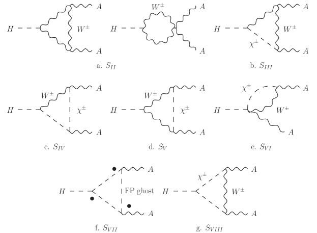
Figure 2: Feynman diagram representation of the effective action obtained from (2)

The second term of (101) contains, apart from (21), (22) and (23), two terms that are reformulated by the Ward identities (18); they are:

$$-iegM_{W}\int d^{4}x\int d^{4}y\int d^{4}zH(x){\cal A}^{\mu}(y)$$

$$G_{{\rm vec},\lambda\rho}(x,y)(-\delta^{\rho}\hskip 0.28453pt_{\mu}D^{\sigma}+\delta^{\sigma}\hskip 0.28453pt_{\mu}\stackrel{{\scriptstyle\leftarrow}}{{D}}^{\rho})G_{{\rm vec},\sigma\omega}(y,z)({\cal H}^{(1)})^{\omega\epsilon}(z)G_{{\rm vec},\epsilon}\hskip 0.28453pt^{\lambda}(z,x)$$

$$-iegM_{W}\int d^{4}x\int d^{4}y\int d^{4}zH(x){\cal A}^{\nu}(z)$$

$$G_{{\rm vec},\lambda\rho}(x,y)({\cal H}^{(1)})^{\rho\sigma}(y)G_{{\rm vec},\sigma\omega}(y,z)(-\delta^{\omega}\hskip 0.28453pt_{\nu}D^{\epsilon}+\delta^{\epsilon}\hskip 0.28453pt_{\nu}\stackrel{{\scriptstyle\leftarrow}}{{D}}^{\omega})G_{{\rm vec},\epsilon}\hskip 0.28453pt^{\lambda}(z,x)$$ (108)

and:

$$-e^{2}gM_{W}\int d^{4}x\int d^{4}y\int d^{4}zH(x){\cal A}^{\mu}(y){\cal A}^{\nu}(z)$$

$$G_{{\rm vec},\lambda\rho}(x,y)(-\delta^{\rho}\hskip 0.28453pt_{\mu}D^{\sigma}+\delta^{\sigma}\hskip 0.28453pt_{\mu}\stackrel{{\scriptstyle\leftarrow}}{{D}}^{\rho})G_{{\rm vec},\sigma\omega}(y,z)(-\delta^{\omega}\hskip 0.28453pt_{\nu}D^{\epsilon}+\delta^{\epsilon}\hskip 0.28453pt_{\nu}\stackrel{{\scriptstyle\leftarrow}}{{D}}^{\omega})G_{{\rm vec},\epsilon}\hskip 0.28453pt^{\lambda}(z,x).$$ (109)

(108) contains by (7):

$$-e^{2}gM_{W}\int d^{4}x\int d^{4}y\int d^{4}zH(x){\cal A}^{\mu}(y){\cal A}^{\nu}(z)$$

$$(G_{{\rm vec},\lambda\mu}(x,y)G_{{\rm sc}}(y,z)(\eta_{\nu\omega}D^{2}-2ieF_{\nu\omega}(z)-D_{\nu}D_{\omega})G_{{\rm vec}}\hskip 0.28453pt^{\omega\lambda}(z,x)$$

$$+G_{{\rm vec},\lambda}\hskip 0.28453pt^{\rho}(x,y)(\stackrel{{\scriptstyle\leftarrow}}{{D}}^{2}\eta_{\rho\mu}-2ieF_{\rho\mu}(y)-\stackrel{{\scriptstyle\leftarrow}}{{D}}_{\rho}\stackrel{{\scriptstyle\leftarrow}}{{D}}_{\ \mu})G_{{\rm sc}}(y,z)G_{{\rm vec},\nu}\hskip 0.28453pt^{\lambda}(z,x)).$$ (110)

The rest of (108) is added to (102), and the sum is by (7) and (18):

$$\frac{1}{2}e^{2}gM_{W}\int d^{4}x\int d^{4}y\int d^{4}zH(x)G_{{\rm sc}}(x,y){\cal A}^{\mu}(y)(\eta_{\mu\lambda}D^{2}-2ieF_{\mu\lambda}(y)-D_{\mu}D_{\lambda})$$

$$G_{{\rm vec}}\hskip 0.28453pt^{\lambda\nu}(y,z){\cal A}_{\nu}(z)G_{{\rm sc}}(z,x)$$

$$+\frac{1}{2}e^{2}gM_{W}\int d^{4}x\int d^{4}y\int d^{4}zH(x)G_{{\rm sc}}(x,y)$$

$${\cal A}_{\mu}(y)G_{{\rm vec}}\hskip 0.28453pt^{\mu\lambda}(y,z)(\eta_{\lambda\nu}\stackrel{{\scriptstyle\leftarrow}}{{D}}^{2}-2ieF_{\lambda\nu}(z)-\stackrel{{\scriptstyle\leftarrow}}{{D}}_{\lambda}\stackrel{{\scriptstyle\leftarrow}}{{D}}_{\nu}){\cal A}^{\nu}(z)G_{{\rm sc}}(z,x).$$ (111)

(110) is by (13) and (18) the sum of:

$$-2ie^{2}gM_{W}\int d^{4}x\int d^{4}yH(x){\cal A}^{\mu}(x)G_{{\rm vec},\mu\nu}(x,y){\cal A}^{\nu}(y)G_{{\rm sc}}(y,x)$$ (112)

and also:

$$2e^{2}gM_{W}^{3}\int d^{4}x\int d^{4}y\int d^{4}zH(x)G_{{\rm vec},\lambda\mu}(x,y){\cal A}^{\mu}(y)G_{{\rm sc}}(y,z){\cal A}^{\nu}(z)G_{{\rm vec},\nu}\hskip 0.28453pt^{\lambda}(z,x)$$ (113)

and:

$$e^{2}gM_{W}\int d^{4}x\int d^{4}y\int d^{4}zH(x){\cal A}^{\mu}(y){\cal A}^{\nu}(z)$$

$$(G_{{\rm vec},\lambda\mu}(x,y)G_{{\rm sc}}(y,z)D_{\nu}G_{{\rm sc}}(z,x)\stackrel{{\scriptstyle\leftarrow}}{{D}}^{\lambda}$$

$$+D_{\lambda}G_{{\rm sc}}(x,y)\stackrel{{\scriptstyle\leftarrow}}{{D}}_{\mu}G_{{\rm sc}}(y,z)G_{{\rm vec},\nu}\hskip 0.28453pt^{\lambda}(z,x)).$$ (114)

Also (111) contains the first term of (24), as well as:

$$-e^{2}gM_{W}^{3}\int d^{4}x\int d^{4}y\int d^{4}zH(x)G_{{\rm sc}}(x,y){\cal A}_{\mu}(y)G_{{\rm vec}}\hskip 0.28453pt^{\mu\nu}(y,z){\cal A}_{\nu}(z)G_{{\rm sc}}(z,x)$$ (115)

and also:

$$e^{2}gM_{W}\int d^{4}x\int d^{4}y\int d^{4}zH(x)G_{{\rm sc}}(x,y){\cal A}^{\mu}(y)D_{\mu}G_{{\rm sc}}(y,z){\cal A}^{\nu}(z)D_{\nu}G_{{\rm sc}}(z,x).$$ (116)

From (109) one gets, again by (18):

$$e^{2}gM_{W}\int d^{4}x\int d^{4}y\int d^{4}zH(x){\cal A}^{\mu}(y){\cal A}^{\nu}(z)$$

$$(G_{{\rm vec},\lambda\mu}(x,y)G_{{\rm sc}}(y,x)D_{\nu}G_{{\rm sc}}(z,x)\stackrel{{\scriptstyle\leftarrow}}{{D}}^{\lambda}$$

$$+D_{\lambda}G_{{\rm sc}}(x,y)\stackrel{{\scriptstyle\leftarrow}}{{D}}_{\mu}G_{{\rm sc}}(y,z)G_{{\rm vec},\nu}\hskip 0.28453pt^{\lambda}(z,x))$$ (117)

that is identical to (114), and:

$$e^{2}gM_{W}\int d^{4}x\int d^{4}y\int d^{4}zH(x)$$

$$D_{\lambda}G_{{\rm sc}}(x,y){\cal A}^{\mu}(y)G_{{\rm vec},\mu\nu}(y,z){\cal A}^{\nu}(z)G_{{\rm sc}}(z,x)\stackrel{{\scriptstyle\leftarrow}}{{D}}^{\lambda}$$ (118)

and also:

$$e^{2}gM_{W}\int d^{4}x\int d^{4}y\int d^{4}zH(x)$$

$$G_{{\rm vec},\lambda\mu}(x,y){\cal A}^{\mu}(y)D^{2}G_{{\rm sc}}(y,z){\cal A}^{\nu}(z)G_{{\rm vec},\nu}\hskip 0.28453pt^{\lambda}(z,x).$$ (119)

(114), (116) and (117) are added to (103) and (106); using again (18) one obtains the second term of (24). Also (118) is by the background Higgs boson field on-shell condition and (11) the sum of:

$$-2\lambda e^{2}M_{W}^{2}v\int d^{4}x\int d^{4}y\int d^{4}zH(x)G_{{\rm sc}}(x,y){\cal A}^{\mu}(y)G_{{\rm vec},\mu\nu}(y,z){\cal A}^{\nu}(z)G_{{\rm sc}}(z,x)$$ (120)

that cancels with (107), as well as:

$$ie^{2}gM_{W}\int d^{4}x\int d^{4}yH(x){\cal A}^{\mu}(x)G_{{\rm vec},\mu\nu}(x,y){\cal A}^{\nu}(y)G_{{\rm sc}}(y,x)$$ (121)

and:

$$e^{2}gM_{W}^{3}\int d^{4}x\int d^{4}y\int d^{4}zH(x)G_{{\rm sc}}(x,y){\cal A}^{\mu}(y)G_{{\rm vec},\mu\nu}(y,z){\cal A}^{\nu}(z)G_{{\rm sc}}(z,x)$$ (122)

that cancels with (115). Finally (119) is by (11) the sum of:

$$-ie^{2}gM_{W}\int d^{4}x\int d^{4}yH(x)G_{{\rm vec},\lambda\mu}(x,y){\cal A}^{\mu}(y){\cal A}^{\nu}(y)G_{{\rm vec},\nu}\hskip 0.28453pt^{\lambda}(y,x)$$ (123)

that cancels the remainder of the first term of (101), and:

$$-e^{2}gM_{W}^{3}\int d^{4}x\int d^{4}y\int d^{4}zH(x)G_{{\rm vec},\lambda\mu}(x,y){\cal A}^{\mu}(y)G_{{\rm sc}}(y,z){\cal A}^{\nu}(z)G_{{\rm vec},\nu}\hskip 0.28453pt^{\lambda}(z,x).$$ (124)

(112) and (121) cancel with (105), and (113) and (124) cancel with (104).

In summary (101), (102), (103), (104), (105), (107) and (106) have been reduced to (21), (22), (23) and (24) that are invariant under gauge transformations of the radiation field ${\cal A}_{\mu}$ as shown in app. C.

Using proper-time regularization one finds additional terms from (110) and (119) by the methods developed in [16]:

$$-ie^{2}gM_{W}\int_{0}^{\infty}d\tau\frac{\partial}{\partial\tau}\bigg{(}\tau^{2}\int_{0}^{1}d\alpha d\beta d\gamma\delta(1-\alpha-\beta-\gamma)$$

$$\int d^{4}x\int d^{4}y\int d^{4}zH(x)h_{{\rm vec},\lambda\mu}(x,y;\alpha\tau){\cal A}^{\mu}(y)h_{{\rm sc}}(y,z;\beta\tau){\cal A}_{\nu}(z)h_{{\rm vec},}\hskip 0.28453pt^{\nu\lambda}(z,x;\gamma\tau)\bigg{)}$$

$$\simeq\frac{1}{32\pi^{2}}e^{2}gM_{W}\int d^{4}xH(x){\cal A}^{\mu}(x){\cal A}_{\mu}(x)$$ (125)

while the corresponding additional terms from (111) and (118) cancel out. (125) is not invariant under a gauge transformation of the radiation field ${\cal A}_{\mu}(x)$ and should be discarded. It seems to be a general deficiency of the proper-time regularization method that such expressions occur and should be eliminated either by hand or by use of dimensional regularization [16].

Appendix B Propagators and kernels in a homogeneous background electromagnetic field

B.1 The scalar kernel in a homogeneous electromagnetic field

The starting point for finding propagators in a homogeneous background field is the scalar kernel determined by Schwinger [5]:

$$<x,\tau\mid x^{\prime},0>=<x\mid e^{-i\tau H}\mid x^{\prime}>;\ <x,\tau\mid=<x\mid e^{-i\tau H}$$ (126)

with the quasi-Hamiltonian:

$$H=-\Pi^{2}=-\eta^{\mu\nu}\Pi_{\mu}\Pi_{\nu}$$ (127)

where $\Pi_{\mu}=-iD_{\mu}=-i(\partial_{\mu}-ieA_{\mu})$. A position operator $X_{\mu}$ is introduced, with:

$$X_{\mu}\mid x>=x_{\mu}\mid x>$$ (128)

such that:

$$[\Pi_{\mu},X_{\nu}]=-i\eta_{\mu\nu},[X_{\mu},X_{\nu}]=0,\ [\Pi_{\mu},\Pi_{\nu}]=ieF_{\mu\nu}.$$ (129)

The field strength $F_{\mu\nu}$ is assumed homogeneous.

$X_{\mu}$ and $\Pi_{\mu}$ can be considered operators in a quasi-Heisenberg picture [5]. Thus their proper-time development is governed by:

$$\frac{dX_{\mu}}{d\tau}=-i[X_{\mu},H]=-2\Pi_{\mu}$$ (130)

and:

$$\frac{d\Pi_{\mu}}{d\tau}=-i[\Pi_{\mu},H]=-2eF_{\mu}^{\nu}\Pi_{\nu}$$ (131)

or in a matrix notation:

$$\frac{dX}{d\tau}=-2\Pi,\ \frac{d\Pi}{d\tau}=-2e{\bf F}\Pi$$ (132)

with solutions:

$$\Pi(\tau)=e^{-2\tau e{\bf F}}\Pi(0),\ X(\tau)=X(0)-{\bf D}(\tau)\Pi(0)$$ (133)

where:

$${\bf D}(\tau)=\frac{{\bf 1}-e^{-2\tau e{\bf F}}}{e{\bf F}}.$$ (134)

From (129) and (133) follows:

$$<x,\tau\mid\Pi_{\mu}\mid x,0>=0,\ <x,\tau\mid\Pi_{\mu}\Pi_{\nu}\mid x,0>=i({\bf D}^{-1}(\tau))_{\mu\nu}<x,\tau\mid x,0>.$$ (135)

The scalar and vector propagators in the Feynman gauge are, cf. (10) and (14):

$$G_{{\rm sc}}(x,x^{\prime})=\int_{0}^{\infty}d\tau e^{-i\tau M_{W}^{2}}<x,\tau\mid x^{\prime},0>,$$

$$G_{{\rm vec},\mu\nu}(x,x^{\prime})=-\int_{0}^{\infty}d\tau e^{-i\tau M_{W}^{2}}(\exp(-2\tau e{\bf F}))_{\mu\nu}<x,\tau\mid x^{\prime},0>$$ (136)

using a matrix notation for the background field strength. The kernel determined by Schwinger is at coinciding points:

$$<x,\tau\mid x,0>=-\frac{i}{16\pi^{2}\tau^{2}}\exp(-\frac{1}{2}{\rm tr}\log\frac{\sinh(\tau e{\bf F})}{\tau e{\bf F}}).$$ (137)

Also one finds from (133):

$$X(\alpha\tau)=({\bf 1}-{\bf D}(\alpha\tau){\bf D}^{-1}(\tau))X(0)+{\bf D}(\alpha\tau){\bf D}^{-1}(\tau)X(\tau)$$ (138)

The Baker-Campbell-Hausdorff identity:

$$e^{a+b}=e^{a}e^{b}e^{-\frac{1}{2}[a,b]},$$ (139)

which is valid when $[a,b]$ commutes with $a$ and $b$, combined with (138), implies [6], [7]:

$$\exp(ik\cdot X(\alpha\tau))=\exp(ik\cdot{\bf D}(\alpha\tau){\bf D}^{-1}(\tau)X(\tau))$$

$$\exp(ik\cdot(1-{\bf D}(\alpha\tau){\bf D}^{-1}(\tau))X(0))e^{\delta_{1}(\alpha,k)}$$ (140)

where:

$$\delta_{1}(\alpha,k)=\frac{1}{2}ik\cdot{\bf D}(\alpha\tau){\bf D}((1-\alpha)\tau){\bf D}^{-1}(\tau)k.$$ (141)

Using again (139) and (140) one gets:

$$\exp(ik\cdot X((1-\alpha)\tau)\exp(iq\cdot X(\gamma\tau))$$

$$=\exp(iQ\cdot X(\tau))\exp(i(k+q-Q)\cdot X(0))e^{\delta_{2}(k,q)}$$ (142)

with:

$$\delta_{2}(k,q)=\frac{1}{2}ik\cdot{\bf D}((1-\alpha)\tau){\bf D}(\alpha\tau){\bf D}^{-1}(\tau)k+\frac{1}{2}iq\cdot{\bf D}((1-\gamma)\tau){\bf D}(\gamma\tau){\bf D}^{-1}(\tau)q$$

$$+iq\cdot{\bf D}(\alpha\tau){\bf D}(\gamma\tau){\bf D}^{-1}(\tau)k$$ (143)

where:

$$\delta_{2}(k,q)\mid_{\gamma=1-\alpha}=\delta_{1}(\alpha,k+q).$$ (144)

For vanishing background field one gets:

$$\delta_{2}(k,q)=i\tau\alpha\gamma M_{H}^{2}$$ (145)

with $k^{2}=q^{2}=0,2kq=M_{H}^{2}$. Also we have defined:

$$Q=({\bf D}((1-\alpha)\tau){\bf D}^{-1}(\tau))^{T}k+({\bf D}(\gamma\tau){\bf D}^{-1}(\tau))^{T}q$$ (146)

where the superscript $T$ denotes transposed matrix, and with:

$$e^{2\alpha\tau e{\bf F}}Q=k-({\bf D}(\alpha\tau){\bf D}(\tau)^{-1})^{T}k+(({\bf D}((\alpha+\gamma)\tau)-{\bf D}(\alpha\tau)){\bf D}(\tau)^{-1})^{T}q$$ (147)

and:

$$e^{-2\gamma\tau e{\bf F}}(k+q-Q)=q-{\bf D}(\gamma\tau){\bf D}(\tau)^{-1}q+({\bf D}((\alpha+\gamma)\tau)-{\bf D}(\gamma\tau)){\bf D}(\tau)^{-1}k.$$ (148)

B.2 A pure magnetic field

In a pure homogeneous magnetic field $B$, which for simplicity is taken along the positive $1$-axis, one gets $F_{2}^{3}=-F_{3}^{2}=-B,\ {\bf F}=-iB{\bf\sigma}_{2}$, with ${\bf{\sigma}}_{2}$ the second Pauli matrix, and (137) is here [5]:

$$<x,\tau\mid x,0>=-\frac{i}{16\pi^{2}\tau^{2}}\frac{\tau eB}{\sin(\tau eB)}.$$ (149)

The apparent singularity at $\tau=\frac{n\pi}{eB},n\epsilon Z$ is spurious since $\tau$ is an integration variable and the integration path can be deformed to run below the real axis or along the negative imaginary axis.

Also one gets here:

$$e^{-2\tau e{\bf F}}=\left(\begin{array}[]{cc}{\bf 1}&{\bf 0}\\ {\bf 0}&\cos(2\tau eB){\bf 1}+i\sin(2\tau eB){\bf\sigma}_{2}\end{array}\right)$$ (152)

From (152) follows:

$${\bf D}(\tau)=\left(\begin{array}[]{cc}2\tau{\bf 1}&{\bf 0}\\ {\bf 0}&\frac{1}{eB}(\sin(2\tau eB){\bf 1}-i(\cos(2\tau eB)-1){\bf\sigma}_{2})\end{array}\right).$$ (155)

One also finds:

$$e^{-2(1-\alpha-\gamma)\tau e{\bf F}}{\bf D}^{-1}(\tau)=\left(\begin{array}[]{cc}\frac{1}{2\tau}{\bf 1}&{\bf 0}\\ {\bf 0}&\frac{eB}{2\sin(\tau eB)}(\cos((1-2(\alpha+\gamma)\tau eB){\bf 1}+i\sin((1-2(\alpha+\gamma))\tau eB)){\bf\sigma}_{2})\end{array}\right)$$ (156)

and:

$${\bf D}(\alpha\tau){\bf D}^{-1}(\tau)=\left(\begin{array}[]{cc}\alpha{\bf 1}&{\bf 0}\\ {\bf 0}&\frac{\sin(\alpha\tau eB)}{\sin(\tau eB)}(\cos((1-\alpha)\tau eB){\bf 1}-i\sin((1-\alpha)\tau eB){\bf\sigma}_{2}\end{array}\right)$$ (157)

and thus:

$${\bf D}(\gamma\tau){\bf D}(\alpha\tau){\bf D}^{-1}(\tau)=\left(\begin{array}[]{cc}2\alpha\gamma\tau{\bf 1}&{\bf 0}\\ {\bf 0}&{\bf X}\end{array}\right)$$ (160)

where:

$${\bf X}=\frac{2\sin(\alpha\tau eB)\sin(\gamma\tau eB)}{eB\sin(\tau eB)}(\cos((1-\alpha-\gamma)\tau eB){\bf 1}-i\sin((1-\alpha-\gamma)\tau eB){\bf\sigma}_{2}).$$ (161)

From (157) follows at $\tau\rightarrow-i\infty,\alpha\simeq\gamma\simeq\frac{1}{2}$:

$${\bf D}(\alpha\tau){\bf D}^{-1}(\tau)\simeq\frac{1}{2}({\bf 1}-\left(\begin{array}[]{cc}{\bf 0}&{\bf 0}\\ {\bf 0}&{\bf\sigma}_{2}\end{array}\right)),$$ (164)

$${\bf D}((\alpha+\gamma)\tau){\bf D}^{-1}(\tau)\simeq{\bf 1}-\frac{1}{2}(1-e^{-2i(1-\alpha-\gamma)\tau eB})\left(\begin{array}[]{cc}{\bf 0}&{\bf 0}\\ {\bf 0}&{\bf 1}+{\bf\sigma}_{2}\end{array}\right)$$ (167)

and (147) and (148) are in this limit for a pure magnetic field:

$$e^{2\alpha\tau e{\bf F}}Q\simeq\frac{1}{2}(k+q-i(0,0,\frac{1}{B}\vec{B}\times\vec{k})-(1-e^{-2i(1-\alpha-\gamma)\tau eB})(0,0,\vec{q}_{\perp})$$

$$-ie^{-2i(1-\alpha-\gamma)\tau eB}(0,0,\frac{1}{B}\vec{B}\times\vec{q}))$$ (168)

and:

$$e^{-2\gamma\tau e{\bf F}}(k+q-Q)\simeq\frac{1}{2}(k+q+i(0,0,\frac{1}{B}\vec{B}\times\vec{q})-(1-e^{-2i(1-\alpha-\gamma)\tau eB})(0,0,\vec{k}_{\perp})$$

$$+ie^{-2i(1-\alpha-\gamma)\tau eB}(0,0,\frac{1}{B}\vec{B}\times\vec{k})).$$ (169)

Here the exponentials are kept in their present form; they vanish at $\alpha+\gamma\neq 1,\tau\rightarrow-i\infty$, but are equal to 1 at $\alpha+\gamma=1$.

In the same limit one gets from (161):

$${\bf X}\simeq-\frac{i}{2eB}((1+e^{-2i(1-\alpha-\gamma)\tau eB}){\bf 1}+(e^{-2i(1-\alpha-\gamma)\tau eB}-1){\bf\sigma}_{2})$$ (170)

and thus from (143):

$$\delta_{2}(k,q)\simeq i\alpha\gamma\tau(M_{H}^{2}+(\vec{q}_{\perp}+\vec{k}_{\perp})^{2})+i(1-\alpha-\gamma)\tau(\alpha\vec{k}_{\perp}^{2}+\gamma\vec{q}_{\perp}^{2})$$

$$-\frac{1}{2eB}(\vec{q}_{\perp}+\vec{k}_{\perp})^{2}-\frac{e^{-i\theta}}{2eB}(e^{-2i(1-\alpha-\gamma)\tau eB}-1)\mid\vec{q}_{\perp}\mid\mid\vec{k}_{\perp}\mid$$ (171)

with $k^{2}=q^{2}=0,2q\cdot k=M_{H}^{2}$ and with:

$$\vec{q}_{\perp}\cdot\vec{k}_{\perp}=\mid\vec{q}_{\perp}\mid\mid\vec{k}_{\perp}\mid\cos\theta,\frac{1}{B}\vec{B}\cdot(\vec{q}\times\vec{k})=\mid\vec{q}_{\perp}\mid\mid\vec{k}_{\perp}\mid\sin\theta.$$ (172)

where $\vec{k}_{\perp}$ and $\vec{q}_{\perp}$ denote the spatial parts of $k$ and $q$ orthogonal to the magnetic field. With the applications in sec. 4 in mind one can in (168) and (169) take $\alpha=\gamma=\frac{1}{2}$ in the non-exponential terms in contrast to (171). Also (141) is in this limit:

$$\delta_{1}(\alpha,k)\simeq i\alpha(1-\alpha)\tau(k^{2}+\vec{k}_{\perp}^{2})-\frac{\vec{k}_{\perp}^{2}}{2eB}.$$ (173)

At $\tau\rightarrow-i\infty$ one gets from (149):

$$<x,\tau\mid x,0>\simeq\frac{1}{8\pi^{2}\tau}eBe^{-i\tau eB}$$ (174)

and (152) is for $\tau\rightarrow-i\infty$ approximately.

$$e^{-2\tau e{\bf F}}\simeq\left(\begin{array}[]{cc}{\bf 1}&{\bf 0}\\ {\bf 0}&{\bf 0}\end{array}\right)+\frac{1}{2}e^{2i\tau eB}\left(\begin{array}[]{cc}{\bf 0}&{\bf 0}\\ {\bf 0}&{\bf 1}+{\bf\sigma}_{2}\end{array}\right).$$ (175)

From (156) one finally gets in this approximation:

$$e^{-2(1-\alpha-\gamma)\tau e{\bf F}}{\bf D}^{-1}(\tau)\simeq\left(\begin{array}[]{cc}\frac{1}{2\tau}{\bf 1}&{\bf 0}\\ {\bf 0}&\frac{1}{2}ieBe^{-2i(1-\alpha-\gamma)\tau eB}({\bf 1}-{\bf\sigma}_{2})\end{array}\right).$$ (178)

Appendix C Invariance of the $H\rightarrow\gamma\gamma$ decay amplitude under gauge transformations of the radiation field

C.1 A general background field

After gauge fixing the radiation field ${\cal A}_{\mu}(x)$ has a residual gauge freedom under the gauge transformation ${\cal A}_{\mu}(x)\rightarrow{\cal A}_{\mu}(x)+\partial_{\mu}\Lambda(x),\ \partial^{2}\Lambda(x)=0$. Doing this gauge transformation on (20) one gets at first order in $\Lambda$:

$$-4i\lambda e^{2}v\int d^{4}x\int d^{4}yH(x)G_{{\rm sc}}(x,y)\partial_{\nu}({\cal A}^{\nu}(y)\Lambda(y))G_{\rm{sc}}(y,x)$$

$$-8\lambda e^{2}v\int d^{4}x\int d^{4}y\int d^{4}zH(x)G_{{\rm sc}}(x,y)(\partial^{\nu}\Lambda)(y)D_{\nu}G_{{\rm sc}}(y,z){\cal A}^{\rho}(z)D_{\rho}G_{{\rm sc}}(z,x)$$

$$-8\lambda e^{2}v\int d^{4}x\int d^{4}y\int d^{4}zH(x)G_{{\rm sc}}(x,y){\cal A}^{\nu}(y)D_{\nu}G_{{\rm sc}}(y,z)(\partial^{\rho}\Lambda)(z)D_{\rho}G_{{\rm sc}}(z,x)$$ (179)

that cancel by partial integration and use of (11). (21) and (24) are invariant under gauge transformations of the radiation field by the same argument. (22) is manifestly invariant. From (23) one gets by a gauge transformation:

$$2ie^{2}gM_{W}\int d^{4}x\int d^{4}y\int d^{4}z\int d^{4}pH(p)e^{ipx}\int d^{4}k{\cal A}^{\mu}(k)e^{iky}\int d^{4}q\Lambda(q)e^{iqz}$$

$$G_{{\rm vec},\lambda\rho}(x,y)(\delta^{\rho}\hskip 0.28453pt_{\mu}k^{\sigma}-\delta^{\sigma}\hskip 0.28453pt_{\mu}k^{\rho})G_{{\rm vec},\sigma\omega}(y,z)(D^{2}-\stackrel{{\scriptstyle\leftarrow}}{{D}}^{2})G_{{\rm vec},}\hskip 0.28453pt^{\omega\lambda}(z,x)$$

$$+2ie^{2}gM_{W}\int d^{4}x\int d^{4}y\int d^{4}z\int d^{4}pH(p)e^{ipx}\int d^{4}k\Lambda(k)e^{iky}\int d^{4}q{\cal A}^{\nu}(q)e^{iqz}$$

$$G_{{\rm vec},\lambda\rho}(x,y(D^{2}-\stackrel{{\scriptstyle\leftarrow}}{{D}}^{2})G_{{\rm vec},}\hskip 0.28453pt^{\rho}\hskip 0.28453pt{}_{\omega}(y,z)(\delta^{\omega}\hskip 0.28453pt_{\nu}q^{\epsilon}-\delta^{\epsilon}\hskip 0.28453pt_{\nu}q^{\omega})G_{{\rm vec},\epsilon}\hskip 0.28453pt^{\lambda}(z,x))$$

$$=0$$ (180)

by (13). Using a proper-time representation in the two last terms of (179) by (10) one finds that the additional term corresponding to (125) vanishes in this case. The additional term from (180) also vanishes.

C.2 Singular terms in a homogeneous magnetic field

It is not obvious that the sum of the singular terms of the amplitude (63), (66) and (67) and also the singular term (83) are invariant under gauge transformations of the photon polarization vectors, and the approximation procedure used to obtain these expressions means that the result of the preceeding subsection does not apply automatically. It is verified below that the approximation procedure indeed respects gauge invariance.

From (63) one first gets through $\varepsilon^{\mu}(k)\rightarrow ik^{\mu}\Lambda(k)$:

$$-\frac{ie^{2}gM_{W}}{4\pi}\Lambda(k)\varepsilon^{\nu}(q)\exp(-\frac{(\vec{k}_{\perp}+\vec{q}_{\perp})^{2}}{2eB})$$

$$\frac{eB}{\sqrt{(M_{H}^{2}+(\vec{k}_{\perp}+\vec{q}_{\perp})^{2})(M_{W}^{2}-eB-\frac{1}{4}(M_{H}^{2}+(\vec{k}_{\perp}+\vec{q}_{\perp})^{2}))}}$$

$$((0,0,\vec{k}_{\perp})_{\nu}+e^{-i\theta}\mid\vec{q}_{\perp}\mid\mid\vec{k}_{\perp}\mid F(1,\theta)((0,0,\vec{k}_{\perp})-i(0,0,\frac{1}{B}\vec{B}\times\vec{q}))_{\nu}$$

$$+e^{i\theta}\mid\vec{q}_{\perp}\mid\mid\vec{k}_{\perp}\mid F(1,-\theta)((0,0,\vec{k}_{\perp})+i(0,0,\frac{1}{B}\vec{B}\times\vec{q}))_{\nu})$$ (181)

by the following identity, which is a consequence of the definition (59):

$$(q\cdot k+\vec{q}_{\perp}\cdot\vec{k}_{\perp})F(j,\theta)=\frac{1}{2}+e^{-i\theta}\mid\vec{q}_{\perp}\mid\mid\vec{k}_{\perp}\mid F(j+1,\theta)-2jeBF(j,\theta)$$ (182)

and also:

$$\frac{ie^{2}gM_{W}}{4\pi}\Lambda(k)k_{\nu}\varepsilon^{\nu}(q)\vec{q}_{\perp}\cdot\vec{k}_{\perp}\exp(-\frac{(\vec{k}_{\perp}+\vec{q}_{\perp})^{2}}{2eB})$$

$$\frac{eB}{\sqrt{(M_{H}^{2}+(\vec{k}_{\perp}+\vec{q}_{\perp})^{2})(M_{W}^{2}-eB-\frac{1}{4}(M_{H}^{2}+(\vec{k}_{\perp}+\vec{q}_{\perp})^{2}))}}$$

$$(F(0,\theta)+F(0,-\theta)).$$ (183)

Using again (59) one also gets from (63):

$$\frac{ie^{2}gM_{W}eB}{4\pi}\Lambda(k)\varepsilon^{\nu}(q)\exp(-\frac{(\vec{k}_{\perp}+\vec{q}_{\perp})^{2}}{2eB})$$

$$\frac{1}{\sqrt{(M_{H}^{2}+(\vec{k}_{\perp}+\vec{q}_{\perp})^{2})(M_{W}^{2}-eB-\frac{1}{4}(M_{H}^{2}+(\vec{k}_{\perp}+\vec{q}_{\perp})^{2}))}}$$

$$((0,0,\vec{k}_{\perp})_{\nu}+e^{-i\theta}\mid\vec{q}_{\perp}\mid\mid\vec{k}_{\perp}\mid F(2,\theta)((0,0,\vec{k}_{\perp})+i(0,0,\frac{1}{B}\vec{B}\times\vec{k}))_{\nu}$$

$$+e^{i\theta}\mid\vec{q}_{\perp}\mid\mid\vec{k}_{\perp}\mid F(2,-\theta)((0,0,\vec{k}_{\perp})-i(0,0,\frac{1}{B}\vec{B}\times\vec{k}))_{\nu}$$

$$-2eBF(1,\theta)((0,0,\vec{k}_{\perp})+i(0,0,\frac{1}{B}\vec{B}\times\vec{k}))_{\nu}$$

$$-2eBF(1,-\theta)((0,0,\vec{k}_{\perp})-i(0,0,\frac{1}{B}\vec{B}\times\vec{k}))_{\nu}).$$ (184)

and the final terms obtained from (63) are:

$$-\frac{ie^{2}gM_{W}eB}{4\pi}\mid\vec{q}_{\perp}\mid\mid\vec{k}_{\perp}\mid\Lambda(k)\varepsilon^{\nu}(q)\exp(-\frac{(\vec{k}_{\perp}+\vec{q}_{\perp})^{2}}{2eB})$$

$$\frac{1}{\sqrt{(M_{H}^{2}+(\vec{k}_{\perp}+\vec{q}_{\perp})^{2})(M_{W}^{2}-eB-\frac{1}{4}(M_{H}^{2}+(\vec{k}_{\perp}+\vec{q}_{\perp})^{2}))}}$$

$$(e^{-i\theta}F(1,\theta)(k-(0,0,\vec{k}_{\perp})+i(0,0,\frac{1}{B}\vec{B}\times\vec{q}))_{\nu})$$

$$+e^{i\theta}F(1,-\theta)(k-(0,0,\vec{k}_{\perp})-i(0,0,\frac{1}{B}\vec{B}\times\vec{q}))_{\nu})\bigg{)}$$ (185)

and also:

$$-\frac{ie^{2}gM_{W}eB}{4\pi}\Lambda(k)\varepsilon^{\nu}(q)\mid\vec{q}_{\perp}\mid\mid\vec{k}_{\perp}\mid\exp(-\frac{(\vec{k}_{\perp}+\vec{q}_{\perp})^{2}}{2eB})$$

$$\frac{1}{\sqrt{(M_{H}^{2}+(\vec{k}_{\perp}+\vec{q}_{\perp})^{2})(M_{W}^{2}-eB-\frac{1}{4}(M_{H}^{2}+(\vec{k}_{\perp}+\vec{q}_{\perp})^{2}))}}$$

$$(e^{-i\theta}F(2,\theta)((0,0,\vec{k}_{\perp})+i(0,0,\frac{1}{B}\vec{B}\times\vec{k}))_{\nu}$$

$$+e^{i\theta}F(2,-\theta)((0,0,\vec{k}_{\perp})-i(0,0,\frac{1}{B}\vec{B}\times\vec{k}))_{\nu}\bigg{)}.$$ (186)

Also one gets from (66):

$$\frac{ie^{2}gM_{W}e^{2}B^{2}}{2\pi}\Lambda(k)\varepsilon^{\nu}(q)\exp(-\frac{(\vec{k}_{\perp}+\vec{q}_{\perp})^{2}}{2eB})$$

$$\frac{1}{\sqrt{(M_{H}^{2}+(\vec{k}_{\perp}+\vec{q}_{\perp})^{2})(M_{W}^{2}-eB-\frac{1}{4}(M_{H}^{2}+(\vec{k}_{\perp}+\vec{q}_{\perp})^{2}))}}$$

$$(F(1,\theta)((0,0,\vec{k}_{\perp})+i(0,0,\frac{1}{B}\vec{B}\times\vec{k}_{\perp}))_{\nu}$$

$$+F(1,-\theta)((0,0,\vec{k}_{\perp})-i(0,0,\frac{1}{B}\vec{B}\times\vec{k}_{\perp}))_{\nu})$$ (187)

and from (67):

$$-\frac{ie^{2}gM_{W}eB}{4\pi}\Lambda(k)k_{\nu}\varepsilon^{\nu}(q)\exp(-\frac{(\vec{k}_{\perp}+\vec{q}_{\perp})^{2}}{2eB})$$

$$\frac{1}{\sqrt{(M_{H}^{2}+(\vec{k}_{\perp}+\vec{q}_{\perp})^{2})(M_{W}^{2}-eB-\frac{1}{4}(M_{H}^{2}+(\vec{k}_{\perp}+\vec{q}_{\perp})^{2}))}}$$

$$(\vec{q}_{\perp}\cdot\vec{k}_{\perp}F(0,\theta)-\mid\vec{q}_{\perp}\mid\mid\vec{k}_{\perp}\mid e^{-i\theta}F(1,\theta)+\vec{q}_{\perp}\cdot\vec{k}_{\perp}F(0,-\theta)-\mid\vec{q}_{\perp}\mid\mid\vec{k}_{\perp}\mid e^{i\theta}F(1,-\theta)).$$

(188)

The sum of (181) and (183)-(188) vanishes.

From (83) one gets through $\varepsilon^{\mu}(k)\rightarrow ik^{\mu}\Lambda(k)$ by (182):

$$-\frac{ie^{2}gM_{W}}{4\pi}\Lambda(k)\varepsilon^{\nu}(q)\left(\begin{array}[]{cc}{\bf 0}&{\bf 0}\\ {\bf 0}&{\bf\sigma}_{2}\end{array}\right)_{\epsilon\omega}(\delta^{\omega}\hskip 0.28453pt_{\nu}q^{\epsilon}-\delta^{\epsilon}\hskip 0.28453pt_{\nu}q^{\omega})\exp(-\frac{(\vec{k}_{\perp}+\vec{q}_{\perp})^{2}}{2eB})$$ (191)

$$\frac{eB}{\sqrt{(M_{H}^{2}+(\vec{k}_{\perp}+\vec{q}_{\perp})^{2})(M_{W}^{2}-eB-\frac{1}{4}(M_{H}^{2}+(\vec{k}_{\perp}+\vec{q}_{\perp})^{2}))}}$$

$$((q\cdot k+\vec{q}_{\perp}\cdot\vec{k}_{\perp})F(0,\theta)-e^{-i\theta}\mid\vec{q}_{\perp}\mid\mid\vec{k}_{\perp}\mid F(1,\theta)$$

$$-(q\cdot k+\vec{q}_{\perp}\cdot\vec{k}_{\perp})F(0,-\theta)+e^{i\theta}\mid\vec{q}_{\perp}\mid\mid\vec{k}_{\perp}\mid F(1,-\theta))$$

$$=0.$$ (192)

Appendix D Heisenberg-Euler amplitude

The decay amplitude obtained from the Heisenberg-Euler effective action [15] and involving a $W^{\pm}$-loop can also be found from (2), (136) and (137):

$$gM_{W}<W^{-\mu}(x)W^{+}_{\mu}(x)>=\frac{igM_{W}}{16\pi^{2}}\int_{0}^{\infty}\frac{d\tau}{\tau^{2}}e^{-i\tau M_{W}^{2}}{\rm tr}(e^{-2e{\bf F}\tau})\exp(-\frac{1}{2}{\rm tr}\log\frac{\sinh(\tau e{\bf F})}{\tau e{\bf F}})$$ (193)

where the field strength F, which is assumed homogeneous, is split according to (4), with the momentum of the radiation field ${\cal A}$ going to zero, and only terms of second order in ${\cal A}$ are kept. Introducing [5]:

$${\cal F}=\frac{1}{4}F_{\mu\nu}F^{\mu\nu},{\cal G}=\frac{1}{8}\epsilon_{\mu\nu\lambda\rho}F_{\mu\nu}F^{\lambda\rho}$$ (194)

with $\epsilon_{\mu\nu\lambda\rho}$ the standard antisymmetric symbol, and the eigenvalues of the matrix ${\bf F}$:

$$(F^{(1)},F^{(2)})=\frac{i}{\sqrt{2}}(\sqrt{{\cal F}+i{\cal G}}\pm\sqrt{{\cal F}-i{\cal G}})$$ (195)

one finds:

$$\exp(-\frac{1}{2}{\rm tr}\log\frac{\sinh(\tau e{\bf F})}{\tau e{\bf F}})=\frac{\tau eF^{(1)}}{\sinh(\tau eF^{(1)})}\frac{\tau eF^{(2)}}{\sinh(\tau eF^{(2)})}$$ (196)

and:

$${\rm tr}(e^{-2e{\bf F}\tau})=2\cosh(2\tau eF^{(1)})+2\cosh(2\tau eF^{(2)})$$ (197)

With the background field a homogeneous magnetic field and with the photons emitted along the field lines the quantity ${\cal G}$ vanishes also after the splitting (4), and ${\cal F}$ will not contain terms where the radiation field multiplies the background field (this will not be the case for general directions of emission). Inserting (196) and (197) into (193) one gets:

$$\frac{igM_{W}}{4\pi^{2}}\int_{0}^{\infty}\frac{d\tau}{\tau^{2}}e^{-i\tau M_{W}^{2}}\frac{\tau e\sqrt{2{\cal F}}}{\sin(\tau e\sqrt{2{\cal F}})}(1-\sin^{2}(\tau e\sqrt{2{\cal F}})).$$ (198)

This expression gets through the splitting ${\cal F}\rightarrow{\cal F}+\delta{\cal F}$ the additional terms at first order in $\delta{\cal F}$:

$$\frac{igM_{W}}{8\pi^{2}}\frac{\delta{\cal F}}{{\cal F}}\int_{0}^{\infty}\frac{d\tau}{\tau^{2}}e^{-i\tau M_{W}^{2}}\frac{\tau e\sqrt{2{\cal F}}}{\sin(\tau e\sqrt{2{\cal F}})}(1-\tau e\sqrt{2{\cal F}}\cot(\tau e\sqrt{2{\cal F}})))$$ (199)

and also:

$$-\frac{igM_{W}}{8\pi^{2}}\frac{\delta{\cal F}}{{\cal F}}\int_{0}^{\infty}\frac{d\tau}{\tau^{2}}e^{-i\tau M_{W}^{2}}\tau e\sqrt{2{\cal F}}\sin(\tau e\sqrt{2{\cal F}})(1-\tau e\sqrt{2{\cal F}}\cot(\tau e\sqrt{2{\cal F}})))$$ (200)

and:

$$-\frac{igM_{W}}{4\pi^{2}}\frac{\delta{\cal F}}{{\cal F}}\int_{0}^{\infty}\frac{d\tau}{\tau^{2}}e^{-i\tau M_{W}^{2}}(\tau e\sqrt{2{\cal F}})^{2}\cos(\tau e\sqrt{2{\cal F}}).$$ (201)

Only (200) and (201) are affected by the quasi-tachyonic field component. They are compared with the relevant part of the decay amplitude determined previously in the limit where the photon momenta and thus the Higgs boson mass go to zero with the photons emitted along the field lines. The polarization vectors are orthogonal to the field lines in this case. Then it follows from (147) and (148) combined with (155) that (44) vanishes, while (45) is by (143) with (155) as well as (149), (152) and (156):

$$-\frac{e^{3}gM_{W}B}{\pi^{2}}\varepsilon^{\mu}(k)\varepsilon_{\mu}(q)\int_{0}^{\infty}\tau d\tau e^{-i\tau M_{W}^{2}}\sin(\tau eB)\int_{0}^{1}d\alpha d\beta d\gamma\delta(1-\alpha-\beta-\gamma)e^{i\tau\alpha\gamma M_{H}^{2}}$$

$$(\frac{eB\cos((1-2\beta)\tau eB)}{\sin(\tau eB)}-\frac{1}{\tau})$$ (202)

that at lowest nontrivial order in $M_{H}^{2}$ is:

$$-\frac{ie^{4}gM_{W}B^{2}}{\pi^{2}}M_{H}^{2}\varepsilon^{\mu}(k)\varepsilon_{\mu}(q)\int_{0}^{\infty}\tau^{2}d\tau e^{-i\tau M_{W}^{2}}$$

$$(\frac{1}{24}\frac{1}{\tau eB}\sin(\tau eB)+\frac{1}{8}\frac{1}{(\tau eB)^{3}}(\tau eB\cos(\tau eB)-\sin(\tau eB)))$$ (203)

which when added to (54) is precisely (200) for this particular case.

From (50) one gets in the same limit by (149) and (152):

$$\frac{ie^{2}gM_{W}}{4\pi^{2}}\int_{0}^{\infty}d\tau e^{-i\tau M_{W}^{2}}\frac{\tau eB}{\sin(\tau eB)}\int_{0}^{1}d\beta(1-\beta)$$

$$\bigg{(}\left(\begin{array}[]{cc}{\bf 1}&{\bf 0}\\ {\bf 0}&\cos(2(1-\beta)\tau eB){\bf 1}+i\sin(2(1-\beta)\tau eB){\bf\sigma}_{2}\end{array}\right)_{\epsilon\rho}{\cal F}^{\rho\sigma}(k)$$ (206)

$$\left(\begin{array}[]{cc}{\bf 1}&{\bf 0}\\ {\bf 0}&\cos(2(\beta\tau eB){\bf 1}+i\sin(2\beta\tau eB){\bf\sigma}_{2}\end{array}\right)_{\sigma\omega}{\cal F}^{\omega\epsilon}(q)$$ (209)

$$+\left(\begin{array}[]{cc}{\bf 1}&{\bf 0}\\ {\bf 0}&\cos(2(1-\beta)\tau eB){\bf 1}+i\sin(2(1-\beta)\tau eB){\bf\sigma}_{2}\end{array}\right)_{\epsilon\rho}{\cal F}^{\rho\sigma}(q)$$ (212)

$$\left(\begin{array}[]{cc}{\bf 1}&{\bf 0}\\ {\bf 0}&\cos(2(\beta\tau eB){\bf 1}+i\sin(2\beta\tau eB){\bf\sigma}_{2}\end{array}\right)_{\sigma\omega}{\cal F}^{\omega\epsilon}(k)\bigg{)}$$ (215)

using the Fourier transform of the radiation field strength (6). With the photons emitted along the field lines and their polarization vectors thus orthogonal to the field lines (215) reduces to:

$$\frac{ie^{2}gM_{W}}{4\pi^{2}}\int_{0}^{\infty}d\tau e^{-i\tau M_{W}^{2}}\cos(\tau eB)$$

$$\bigg{(}{\cal F}^{\omega\epsilon}(k)\left(\begin{array}[]{cc}{\bf 1}&{\bf 0}\\ {\bf 0}&{\bf 0}\end{array}\right)_{\epsilon\rho}{\cal F}^{\rho\sigma}(q)\left(\begin{array}[]{cc}{\bf 0}&{\bf 0}\\ {\bf 0}&{\bf 1}\end{array}\right)_{\sigma\omega}+{\cal F}^{\omega\epsilon}(q)\left(\begin{array}[]{cc}{\bf 1}&{\bf 0}\\ {\bf 0}&{\bf 0}\end{array}\right)_{\epsilon\rho}{\cal F}^{\rho\sigma}(k)\left(\begin{array}[]{cc}{\bf 0}&{\bf 0}\\ {\bf 0}&{\bf 1}\end{array}\right)_{\sigma\omega}\bigg{)}$$ (224)

(225)

which is a special case of (201).

The square-root singularity of (1) is not obtained from (200) or (201).