Deconfinement phase transition in the Hamiltonian approach to Yang–Mills theory in Coulomb gauge

Abstract

Recent results obtained for the deconfinement phase transition within the Hamiltonian approach to Yang–Mills theory are reviewed. Assuming a quasiparticle picture for the grand canonical gluon ensemble the thermal equilibrium state is found by minimizing the free energy with respect to the quasi-gluon energy. The deconfinement phase transition is accompanied by a drastic change of the infrared exponents of the ghost and gluon propagators. Above the phase transition the ghost form factor remains infrared divergent but its infrared exponent is approximately halved. The gluon energy being infrared divergent in the confined phase becomes infrared finite in the deconfined phase. Furthermore, the effective potential of the order parameter for confinement is calculated for SU$(N)$ Yang–Mills theory in the Hamiltonian approach by compactifying one spatial dimension and using a background gauge fixing. In the simplest truncation, neglecting the ghost and using the ultraviolet form of the gluon energy, we recover the Weiss potential. From the full non-perturbative potential (with the ghost included) we extract a critical temperature of the deconfinement phase transition of $269$ MeV for the gauge group SU$(2)$ and $283$ MeV for SU$(3)$.

1 Introduction

One of the most challenging problems in particle physics is the understanding of the phase diagram of strongly interacting matter. By means of ultra-relativistic heavy ion collisions the properties of hadronic matter at high temperature and/or density can be explored. From the theoretical point of view we have access to the finite-temperature behavior of QCD by means of lattice Monte-Carlo calculations. This method fails, however, to describe baryonic matter at high density or, more technically, QCD at large chemical baryon potential. Therefore alternative, non-perturbative approaches to QCD which do not rely on the lattice formulation and hence do not suffer from the notorious sign problem are desirable. In recent years much effort has been devoted to develop continuum non-perturbative approaches. Among these is a variational approach to the Hamilton formulation of QCD. In this talk I will summarize the basic results obtained within this approach on the finite-temperature behavior of Yang–Mills theory and, in particular, on the deconfinement phase transition. I will first summarize the basic ingredients of the Hamiltonian approach to Yang–Mills theory and review the essential results obtained at zero temperature. Then I will consider the grand canonical ensemble of Yang–Mills theory and study the deconfinement phase transition. Finally, I will review results obtained for the Polyakov loop, which is the order parameter of confinement. In particular, I will present the effective potential of this order parameter from which I extract the critical temperature of the deconfinement phase transition.

2 Hamiltonian approach to Yang–Mills theory

The Hamiltonian approach to Yang–Mills theory starts from Weyl gauge $A_{0}(x)=0$ and considers the spatial components of the gauge field $A_{i}^{a}(x)$ as coordinates. The momenta are introduced in the standard fashion $\pi^{a}_{i}(x)=\delta S_{\mathrm{YM}}[A]/\delta\dot{A}^{a}_{i}(x)=E^{a}_{i}(x)$ and turn out to be the color electric field ${\bm{\mathrm{E}}}^{a}(x)$. The classical Yang–Mills Hamiltonian is then obtained as

$$H=\frac{1}{2}\int d^{3}x\left(\bm{\mathrm{E}}^{2}(x)+{\bm{\mathrm{B}}}^{2}(x)\right)\,,$$ (1)

where ${\bm{\mathrm{B}}}^{a}(x)$ is the non-Abelian color magnetic field. The theory is quantized by replacing the classical momentum $\pi^{a}_{i}$ by the operator $\Pi^{a}_{i}(x)=-\mathrm{i}\delta/\delta A^{a}_{i}(x)$. The central issue is then to solve the Schrödinger equation $H\psi[A]=E\psi[A]$ for the vacuum wave functional $\psi[A]$. Due to the use of Weyl gauge Gauss’ law $D\Pi\psi[A]=0$ (with $D=\partial+gA$ being the covariant derivative in the adjoint representation) has to be put as a constraint on the wave functional, which ensures the gauge invariance of the latter. Instead of working with explicitly gauge invariant states it is more convenient to fix the gauge and explicitly resolve Gauss’ law in the gauge chosen. For this purpose Coulomb gauge $\bm{\mathrm{\partial}}\bm{\mathrm{A}}=0$ turns out to be particularly convenient. The prise one pays for the gauge-fixing is that the gauge fixed Hamiltonian gets more complicated. In Coulomb gauge it reads

$$H=\frac{1}{2}\int d^{3}x\left(J_{A}^{-1}\,\bm{\mathrm{\Pi}}^{\perp}J_{A}\,\bm{\mathrm{\Pi}}^{\perp}+{\bm{\mathrm{B}}}^{2}[A^{\perp}]\right)+H_{\mathrm{C}}\,,$$ (2)

where $J_{A}=\operatorname{Det}(-D\partial)$ is the Faddeev–Popov determinant and ${\bm{\mathrm{A}}}^{\perp}$ the transversal gauge field. Furthermore,

$$H_{\mathrm{C}}=\frac{g^{2}}{2}\int d^{3}xJ_{A}^{-1}\rho\,(-D\partial)^{-1}(-\partial^{2})(-D\partial)^{-1}J_{A}\,\rho$$ (3)

is the so-called Coulomb term with $\rho^{a}=-\hat{A}^{\perp\,{ab}}_{i}\Pi^{b}_{i}$ being the color charge density of the gauge field. When fermions are included the color charge density contains in addition the part of the quark field. The Faddeev–Popov determinant occurs also in the measure of the scalar product of wave functionals

$$\langle\Phi|\ldots|\Psi\rangle=\int{\cal D}A^{\perp}J_{A}\Phi^{*}[A^{\perp}]\ldots\Psi[A^{\perp}]\,.$$ (4)

Solving the Schrödinger equation within the familiar Rayleigh–Schrödinger perturbation theory yields in leading order the well known $\beta$-function of Yang–Mills theory Campagnari:2009km . Here we are interested in a non-perturbative solution of the Schrödinger equation, for which we use the variational principle with the following trial ansatz for the wave functional FeuRei04

$$\psi[A]=\frac{1}{\sqrt{J[A^{\perp}]}}\exp\left[-\frac{1}{2}\int dx\,dy\,A^{\perp}(x)\,\omega(x,y)\,A^{\perp}(y)\right]\,.$$ (5)

Here $\omega(x,y)$ is a variational kernel, which is determined from the minimization of the energy $\langle\psi|H|\psi\rangle\to min$. For this wave functional the static gluon propagator $D$ acquires the form

$$D(x,y)=\langle A^{\perp}(x)A^{\perp}(y)\rangle=\omega^{-1}(x,y)/2\,,$$ (6)

which defines the Fourier transform of $\omega(x,y)$ as the gluon energy. Minimization of $\langle H\rangle$ with respect to $\omega(x,y)$ yields the result shown in figure 1.

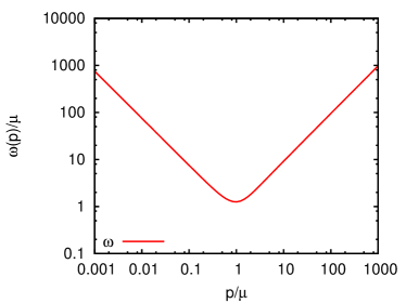
Figure 1: (a) The gluon energy $\omega(p)$ obtained from the minimization of the energy with the trial wave functional (5) Epple:2006hv . (b) Comparison of the static gluon propagator obtained in the variational approach with the lattice data.

At large momenta the gluon energy $\omega(p)$ raises linearly like the photon energy, however, in the infrared it diverges like $\omega_{\mathrm{IR}}(p)\sim 1/p$, which is a manifestation of confinement, i.e. the absence of gluons in the infrared. Figure 1 compares the result of the variational calculation with the lattice results for the gluon propagator. The lattice results can be nicely fitted by Gribov’s formula

$$\omega(p)=\sqrt{p^{2}+M^{4}/p^{2}}$$ (7)

with a mass scale of $M\simeq 880$ MeV. The gluon energy (dashed line) obtained with the Gaussian trial wave functional agrees quite well with the lattice data in the infrared and in the UV-regime but misses some strength in the mid-momentum regime. This missing strength is largely recovered when a non-Gaussian wave functional is used Campagnari:2010wc .

Figure 2: Static quark-antiquark potential Epple:2006hv .

Figure 2 shows the static quark-antiquark potential obtained from the vacuum expectation value of the Coulomb Hamiltonian (3) Epple:2006hv . It rises linearly at large distances, with a coefficient given by the so-called Coulomb string tension $\sigma_{c}$, which on the lattice is measured to be a factor of $2\ldots 3$ larger than the Wilsonian string tension. At small distances it behaves like the Coulomb potential as expected from asymptotic freedom. The Coulomb term (3) turns out to be irrelevant for the Yang–Mills sector. If one further ignores the so-called tadpole [fig. 3] the gap equation, which follows from the minimization of the energy with respect to $\omega$, has the simple form

$$\omega^{2}(p)=p^{2}+\chi^{2}(p)\,,$$ (8)

which is reminiscent to a dispersion relation of a relativistic particle with an effective mass given by the ghost loop $\chi=-\frac{1}{2}\left\langle\frac{\delta^{2}\ln J[A]}{\delta A\delta A}\right\rangle$ shown in fig. 3.

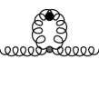
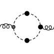
Figure 3: (a) Tadpole diagram, (b) Ghost loop $\chi$.

$$\parbox{56.9055pt}{\includegraphics[width=56.9055pt]{fullghost.ps}}^{-1}\,=\,\parbox{56.9055pt}{\includegraphics[width=56.9055pt]{bareghost.ps}}^{-1}\,-\,\parbox{56.9055pt}{\includegraphics[width=56.9055pt]{ghostgluonloop.ps}}$$

Figure 4: Dyson–Schwinger equation for ghost propagator.

The gap equation (8) has to be solved together with the Dyson–Schwinger equation for the ghost propagator [fig. 4]

$$\langle(-\hat{D}\partial)^{-1}\rangle=d(-\Delta)/(-\Delta)\,.$$ (9)

Here the ghost form factor $d(-\Delta)$ contains all the deviations of QCD from QED. (In QED the ghost propagator is given by $(-\Delta)^{-1}$ so that $d(p)=1$.) Figure 5 shows the solution of the Dyson–Schwinger equation for the ghost form factor. It diverges for $p\to 0$ and approaches asymptotically one in agreement with asymptotic freedom.

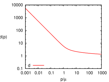
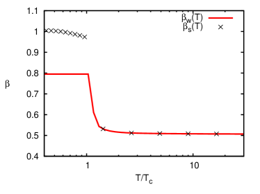
Figure 5: Ghost form factor $d$ at zero temperature (a) and the infrared exponent $\beta$ of the ghost form factor as a function of temperature (b) HefReiCam12 .

The inverse of the ghost form factor can be shown to represent the dielectric function of the Yang–Mills vacuum Reinhardt:2008ek and the so-called horizon condition, which is a necessary condition for confinement, guarantees that this function vanishes in the infrared $\varepsilon(p=0)$, which means that the Yang–Mills vacuum is a perfect color dielectricum, i.e. a dual superconductor. We obtain here precisely the picture which is behind the MIT bag model: At small distances inside the bag the dielectric constant is $1$ corresponding to trivial vacuum while outside the bag the dielectric constant vanishes, which guarantees by the classical Gauss’law $\partial(\varepsilon E)=\rho_{free}$, the absence of three color charges, which is nothing but confinement. Note also that in the whole momentum regime the dielectric function is smaller than $1$, which implies anti-screening.

3 Hamiltonian approach to Yang–Mills theory at finite temperature

The Hamiltonian approach can be straightforwardly extended to finite-temperature Yang–Mills theory by studying the grand canonical ensemble with vanishing gluon chemical potential and minimizing the free energy instead of the vacuum energy. For this purpose one constructs a complete basis of the gluonic Fock space by identifying the trial state (5) as the vacuum state of the gluonic Fock space. Furthermore, assumes a single-particle density operator. Variation of the free energy with respect to the kernel $\omega(p)$ yields the same gap equation (8) as in the zero temperature case except that the ghost loop $\chi(p)$ is now calculated with the finite-temperature ghost propagator, which is obtained from the same Dyson–Schwinger equation as before, see fig. 5, except that also the gluon propagator has to be replaced by its finite-temperature counter part, which is given by

$$D(p)=\frac{1}{2\omega(p)}\left(1+2n(p)\right)\,.$$ (10)

Here

$$n(p)=\left(\exp(\beta\omega(p))-1\right)^{-1}$$ (11)

are the finite-temperature gluon occupation numbers. The two coupled equations (ghost DSE and gap equation) can be solved analytically in the ultraviolet as well as in the infrared at zero and infinite temperature. For this purpose one makes the power law ansätze $\omega(p)=A/p^{\alpha}$, $d(p)=B/p^{\beta}$ for the gluon energy $\omega(p)$ and the ghost form factor $d(p)$. Assuming a bare ghost-gluon vertex one finds the following sum rule for the infrared exponents

$$\alpha=2\beta+2-d\,,$$ (12)

where $d$ is the number of spatial dimensions. From the equations of motion one finds in $d=3$ the following solutions for the infrared exponent of the ghost form factor

$$d=3 :\quad\quad\beta=1\,,\quad\quad\beta\approx 0.795\,,$$

$$d=2 :\quad\quad\beta=1/2\,,$$ (13)

for $d=3$ and $d=2$ spatial dimensions, respectively.

At arbitrary finite temperature an infrared analysis is impossible due to the fact that the gluon energy $\omega(p)$ enters the finite-temperatures occupation numbers $n(p)$ (11) exponentially. However, at infinitely high temperature these occupation numbers $n(p)$ (11) simplify to $n(p)\simeq 1/\beta\omega(p)$. For the infrared exponent one finds then still the same sum rule (12), however, the equations of motions yield now in $d=3$ spatial dimensions only a single solution with $\beta=1/2$, which is precisely the solution for two spatial dimensions at zero temperature, see eq. (3). By the sum rule (12) this implies an infrared finite gluon energy, which corresponds to a massive gluon propagator. Figure 5 shows the infrared exponent of the ghost form factor as function of the temperature as obtained from the numerical solution of the coupled gap equation (8) and ghost Dyson–Schwinger equation (9). As one observes, the two solutions existing at low temperatures merge at a critical temperature $T_{c}$ and eventually approach the high temperature value $\beta=1/2$. Figure 6 shows the numerical solution for the ghost form factor and the gluon energy for temperatures below and above $T_{c}$. The obtained results are in agreement with the analytically performed infrared analysis. Using the Gribov mass in the gluon energy (7) to fix the scale one finds a critical temperature in the range $T_{c}=275\ldots 290$ MeV, see ref. HefReiCam12 for more details.

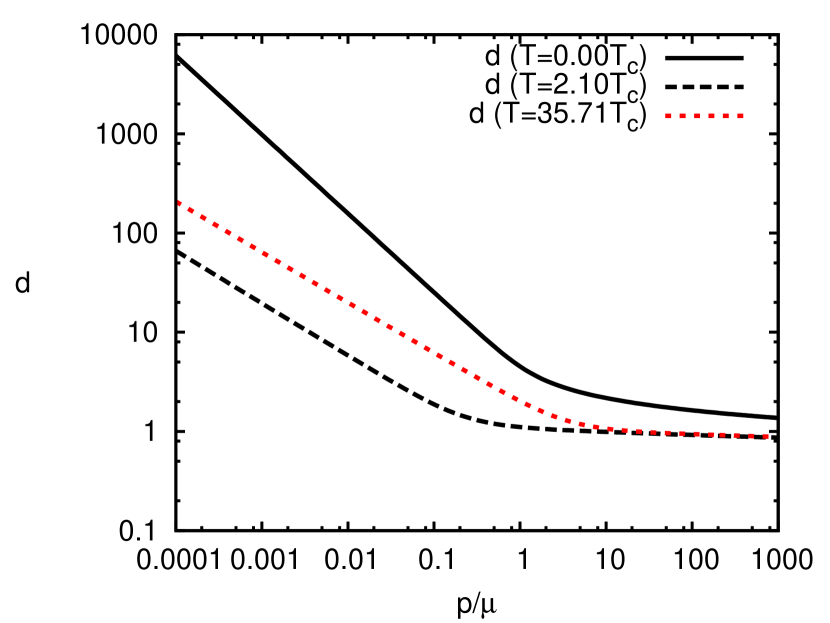
Figure 6: Zero- and finite-temperature solutions for the ghost form factor $d(p)$ (left panel) and the gluon kernel $\omega(p)$ (right panel).

4 The Polyakov loop potential

An alternative way to determine the critical temperature is by means of the Polyakov loop, which we will consider now.

In the standard path integral formulation of a quantum field theory temperature is introduced by continuing the time to purely imaginary values and compactifying the Euclidean time axis to a circle. The circumference $L$ of the circle defines the inverse temperature. The Polyakov loop is then defined by

$$P[A_{0}]({\bm{\mathrm{x}}})=\frac{1}{N}\operatorname{tr}{\cal P}\exp\left[\mathrm{i}\int^{L}_{0}dx_{0}A_{0}(x_{0},{\bm{\mathrm{x}}})\right]\,.$$ (14)

It is just the Wilson line along the compactified Euclidean time direction. The expectation value of this quantity can be shown be related to the free energy $F_{\infty}({\bm{\mathrm{x}}})$ of an isolated static quark by $\langle P[A_{0}]({\bm{\mathrm{x}}})\rangle\sim\exp\left(-LF_{\infty}({\bm{\mathrm{x}}})\right)$. In the confined phase $\langle P[A_{0}]({\bm{\mathrm{x}}})\rangle$ vanishes due to center symmetry while in the deconfined phase, where center symmetry is broken, $F_{\infty}({\bm{\mathrm{x}}})$ is finite and thus $\langle P[A_{0}]({\bm{\mathrm{x}}})\rangle$ is non-zero.

In the continuum theory the Polyakov loop can be most easily calculated in Polyakov gauge defined by $\partial_{0}A_{0}=0$, $A_{0}=\mbox{diagonal}$. In the fundamental modular region $0<A_{0}L/2<\pi$ of this gauge $P[A_{0}]$ is a unique function of $A_{0}$ at least for the gauge groups SU$(2)$ and SU$(3)$. Instead of $\langle P[A_{0}]\rangle$ one can also use $P[\langle A_{0}\rangle]$ and $\langle A_{0}\rangle$ as alternative order parameters of confinement Marhauser:2008fz ; Braun:2007bx . The easiest way to obtain the order parameter of confinement is therefore to do a background field calculation where the background field $a_{0}$ is chosen to agree with the expectation value of the gauge field $\langle A_{0}\rangle$ and furthermore to satisfy Polyakov gauge. From the minimum $a_{0}^{\mathrm{min}}$ of the corresponding effective potential one obtains the order parameter as $\langle P[A_{0}]\rangle\simeq P[a_{0}^{\mathrm{min}}]$. Such a background field calculation has been done long time ago in one-loop perturbation theory Gross:1980br ; Weiss:1980rj , which yields the potential shown in figure 8, which is referred nowadays as Weiss potential. From the minimum $a_{0}^{\mathrm{min}}=0$ of this potential one finds $P[a_{0}^{\mathrm{min}}=0]=1$ corresponding to the deconfined phase. Here we use the Hamiltonian approach to evaluate the effective potential $e[a_{0}]$ non-perturbatively Reinhardt:2012qe ; Reinhardt:2013iia .

Figure 7: The Weiss potential $e_{\text{UV}}$ (18).

Figure 8: The infrared potential $e_{\text{IR}}$ (19).

Since the Hamiltonian approach assumes Weyl gauge $A_{0}(x)=0$ one obviously faces a problem. However, one can exploit O$(4)$ invariance of Euclidean Yang–Mills theory and compactify instead of the time one spatial axis to a circle and interprete the circumference of the circle as the inverse temperature. I will compactify the $3$-axis and choose the background field in the form ${\bm{\mathrm{a}}}=a{\bm{\mathrm{e}}}_{3}$ The calculation of the effective potential $e(a,L)$ in the Hamiltonian approach was for the first time done in ref. Reinhardt:2012qe for the gauge group SU$(2)$ and in ref. Reinhardt:2013iia for SU$(3)$, where also details of the derivation can be found. One finds the following result

$$e(a,L)=\sum_{\sigma}\frac{1}{L}\sum^{\infty}_{n=-\infty}\int\frac{d^{2}p_{\perp}}{(2\pi)^{2}}(\omega(p^{\sigma})-\chi(p^{\sigma}))\,,$$ (15)

where $\omega(p)$ and $\chi(p)$ are the gluon energy and the ghost loop in Coulomb gauge at zero temperature, which, however, have to be taken here at the momentum argument shifted by the background field

$${\bm{\mathrm{p}}}^{\sigma}={\bm{\mathrm{p}}}_{\perp}+\left(p_{n}-{\bm{\mathrm{\sigma}}}\cdot{\bm{\mathrm{a}}}\right){\bm{\mathrm{e}}}_{3}\,,\quad\quad p_{n}=\frac{2\pi n}{L}\,.$$ (16)

Here $p_{n}$ is the Matsubara frequency of the compactified dimension and ${\bm{\mathrm{p}}}_{\perp}$ is the momentum perpendicular to the compactified direction. Furthermore, ${\bm{\mathrm{\sigma}}}$ are the root vectors of the algebra of the gauge group. This potential has the required periodicity property

$$e(a,L)=e(a+\mu_{k}/L,L)\,,$$ (17)

where $\mu_{k}$ denotes the co-weights of the gauge algebra. Its exponentials defines the center elements of the gauge group $\exp(\mathrm{i}\mu_{k})=z_{k}\in\mathrm{Z}(N)$.

Figure 9: The full effective potential for SU$(2)$ for different temperatures $L^{-1}$.

Figure 10: The Polyakov loop $P[a^{\text{min}}]$ calculated at the minimum $a=a^{\text{min}}$ of the effective potential for SU($2$) as a function of $T/T_{c}$.

The expression (15) for the effective potential is surprisingly simple and requires only the knowledge of the gluon energy $\omega(p)$ and the ghost loop $\chi(p)$ in Coulomb gauge at zero temperature.

Before I present the full potential let me first ignore the ghost loop $\chi(p)=0$. The potential (15) becomes then the energy density of a non-interacting Bose gas with single-particle energy $\omega(p)$, living, however, on the spatial manifold $\mathbbm{R}^{2}\times S^{1}$. With $\chi(p)=0$ and replacing the gluon energy $\omega(p)$ (7) by its ultraviolet part $\omega_{\mathrm{UV}}(p)=|{\bm{\mathrm{p}}}|$ one obtains precisely the Weiss potential Reinhardt:2012qe ; Reinhardt:2013iia

$$e_{\mathrm{UV}}(a,L)=\frac{8}{\pi^{2}}\frac{1}{L^{4}}\sum_{\sigma>0}\sum^{\infty}_{n=1}\frac{\sin^{2}\left(n{\bm{\mathrm{a}}}\bm{\mathrm{\sigma}}{L}/{2}\right)}{n^{4}}=\frac{4}{3}\frac{\pi^{2}}{L^{4}}\sum_{\sigma>0}\left(\frac{{\bm{\mathrm{a}}}\bm{\mathrm{\sigma}}L}{2\pi}\right)^{2}\left(\frac{{\bm{\mathrm{a}}}\bm{\mathrm{\sigma}}L}{2\pi}-1\right)^{2}\,,$$ (18)

corresponding to the deconfined phase. Here and in (19) the last expression holds only for $({\bm{\mathrm{a}}}\bm{\mathrm{\sigma}}L/(2\pi))\mod 1$. If on the other hand one chooses the infrared form of the gluon energy (7) $\omega_{\mathrm{IR}}(p)=\frac{M^{2}}{|{\bm{\mathrm{p}}}|}$ one obtains the potential

$$e_{\mathrm{IR}}(a,L)=-4\frac{M^{2}}{\pi^{2}}\frac{1}{L^{2}}\sum_{\sigma>0}\sum^{\infty}_{n=1}\frac{\sin^{2}\left(n{\bm{\mathrm{a}}}\bm{\mathrm{\sigma}}{L}/{2}\right)}{n^{2}}=2\frac{M^{2}}{L^{2}}\sum_{\sigma>0}\left(\left(\frac{{\bm{\mathrm{a}}}\bm{\mathrm{\sigma}}L}{2\pi}\right)^{2}-\frac{{\bm{\mathrm{a}}}\bm{\mathrm{\sigma}}L}{2\pi}\right)\,,$$ (19)

which is shown in figure 8, whose minimum occurs at the center symmetric configuration, which yields a vanishing Polyakov loop corresponding to the confined phase. Obviously, the deconfinement phase transition results from the interplay between the confining IR-potential and the deconfining UV-potentials. Choosing $\omega(p)=\omega_{\mathrm{IR}}(p)+\omega_{\mathrm{UV}}(p)$, which can be considered as an approximation to the Gribov formula (7), one has to add the UV- and IR-potentials, given by eqs. (18) and (19), respectively, and finds a phase transition at a critical temperature $T_{c}=\sqrt{3}M/\pi$. With the Gribov mass $M\simeq 880$ MeV this gives a critical temperature of $T_{c}\approx 485$ MeV, which is much too high. One can show analytically, see ref. Reinhardt:2012qe ; Reinhardt:2013iia , that the neglect of the ghost loop $\chi(p)=0$ shifts the critical temperature to higher values. If one uses eq. (7) for $\omega(p)$ and includes the ghost loop one finds the effective potential shown in fig. 10, which gives a transition temperature $T_{c}\approx 269$ MeV for SU$(2)$, which is in the right ballpark.

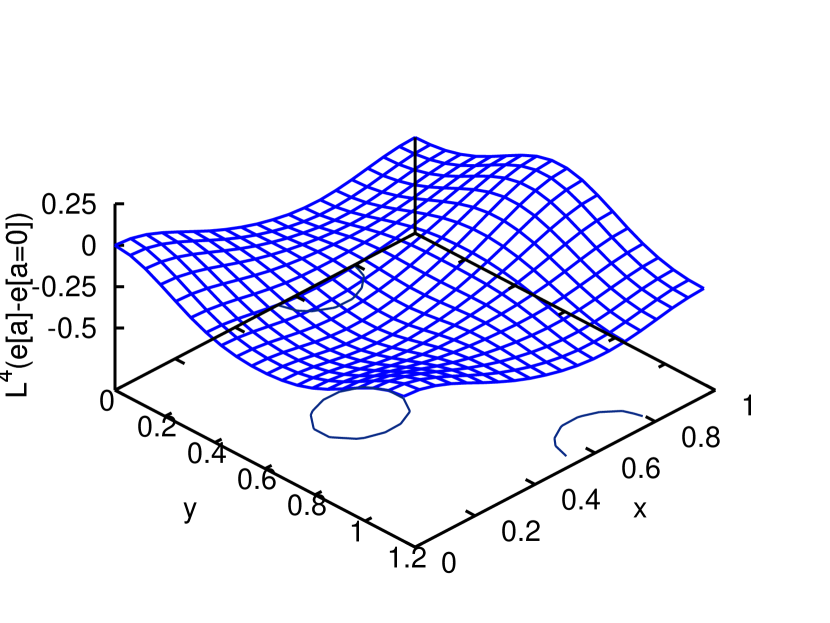
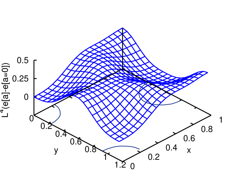
Figure 11: SU$(3)$ effective potential below (left panel) and above (right panel) $T_{c}$ as functions of $x=a_{3}L/(2\pi)$ and $y=a_{8}L/(2\pi)$.

The Polyakov loop $P[a^{\text{min}}]$ calculated from the minimum $a^{\text{min}}$ of the effective potential $e(a,L)$ is plotted in fig. 10 as a function of the temperature.

The effective potential for the gauge group SU$(3)$ can be reduced to that of the SU$(2)$ group by noticing that the SU$(3)$ algebra consist of three SU$(2)$ subalgebras characterized by the three positive roots ${\bm{\mathrm{\sigma}}}=(1,0),\,\left(\frac{1}{2},\frac{1}{2\sqrt{3}}\right),\,\left(\frac{1}{2},-\frac{1}{2\sqrt{3}}\right)$ resulting in

$$e_{\text{SU}(3)}(a)=\sum_{\sigma>0}e_{\text{SU}(2)}[\sigma](a)\,.$$ (20)

The effective potential for SU$(3)$ is shown in fig. 11 as a function of $a_{3}$, $a_{8}$. As one notices, above and below $T_{c}$ the minima of the potential occur in both cases for $a_{8}=0$. Cutting the $2$-dimensional surfaces at $a_{8}=0$ one finds the effective potential shown in fig. 13. This shows a first order phase transition, which occurs at a critical temperature of $T_{c}=283$ MeV. The first order nature of the SU($3$) phase transition is also seen in fig. 13 where the Polyakov loop $P[a^{\text{min}}]$ is shown. Finally let us also mention recent work on the Polyakov loop in alternative continuum approaches Fister:2013bh ; Haas:2013qwp ; Fischer:2013eca ; Smith:2013msa or on the lattice Langelage:2010yr ; Diakonov:2012dx ; Greensite:2012dy ; Greensite:2013yd .

Figure 12: SU($3$) effective potential, cut at $a_{8}=0$, for different temperatures $L^{-1}$.

Figure 13: The Polyakov loop $P[a^{\text{min}}]$ calculated at the minimum $a=a^{\text{min}}$ of the effective potential for SU($3$) as a function of $T/T_{c}$.

5 Conclusions

In my talk I have shown that the Hamiltonian approach in Coulomb gauge gives a decent description of the infrared properties of Yang–Mills theory and at the same time can be extended to finite temperatures where it yields critical temperatures for the deconfinement phase transition in the right ballpark. Furthermore, I have shown that the effective potential of the Polyakov loop can be obtained form the zero-temperature energy density by compactifying one spatial dimension. This potential yields also the correct order of the deconfinement phase transition for SU$(2)$ and SU$(3)$. Presently the Hamiltonian approach in Coulomb gauge is extended to full QCD Pak:2011wu ; Pak:2013uba . After extending the approach to full QCD we plan to consider the influence of an external magnetic field and to study the phase diagram at finite baryon density.

References

- (1) D. R. Campagnari, H. Reinhardt and A. Weber, Phys. Rev. D 80, 025005 (2009).
- (2) C. Feuchter and H. Reinhardt, Phys. Rev. D 70, 105021 (2004), hep-th/0402106.
- (3) D. R. Campagnari and H. Reinhardt, Phys. Rev. D 82, 105021 (2010).
- (4) D. Epple, H. Reinhardt and W. Schleifenbaum, Phys. Rev. D 75, 045011 (2007).
- (5) J. Heffner, H. Reinhardt and D. R. Campagnari, Phys. Rev. D 85, 125029 (2012).
- (6) H. Reinhardt, Phys. Rev. Lett. 101, 061602 (2008).
- (7) F. Marhauser and J. M. Pawlowski, arXiv:0812.1144 [hep-ph].
- (8) J. Braun, H. Gies and J. M. Pawlowski, Phys. Lett. B 684, 262 (2010).
- (9) D. J. Gross, R. D. Pisarski and L. G. Yaffe, Rev. Mod. Phys. 53, 43 (1981).
- (10) N. Weiss, Phys. Rev. D 24, 475 (1981).
- (11) H. Reinhardt and J. Heffner, Phys. Lett. B 718, 2 (2012).
- (12) H. Reinhardt and J. Heffner, Phys. Rev. D 88, 045024 (2013).
- (13) L. Fister and J. M. Pawlowski, Phys. Rev. D 88, 045010 (2013).
- (14) L. M. Haas, R. Stiele, J. Braun, J. M. Pawlowski and J. Schaffner-Bielich, Phys. Rev. D 87, 076004 (2013).
- (15) C. S. Fischer, L. Fister, J. Luecker and J. M. Pawlowski, arXiv:1306.6022 [hep-ph].
- (16) D. Smith, A. Dumitru, R. Pisarski and L. von Smekal, Phys. Rev. D 88, 054020 (2013).
- (17) J. Langelage, S. Lottini and O. Philipsen, JHEP 1102, 057 (2011).
- (18) D. Diakonov, C. Gattringer and H. -P. Schadler, JHEP 1208, 128 (2012).
- (19) J. Greensite, Phys. Rev. D 86, 114507 (2012).
- (20) J. Greensite and K. Langfeld, Phys. Rev. D 87, 094501 (2013).
- (21) M. Pak and H. Reinhardt, Phys. Lett. B 707, 566 (2012).
- (22) M. Pak and H. Reinhardt, arXiv:1310.1797 [hep-ph].