OverFeat:
Integrated Recognition, Localization and Detection
using Convolutional Networks

Abstract

We present an integrated framework for using Convolutional Networks for classification, localization and detection. We show how a multiscale and sliding window approach can be efficiently implemented within a ConvNet. We also introduce a novel deep learning approach to localization by learning to predict object boundaries. Bounding boxes are then accumulated rather than suppressed in order to increase detection confidence. We show that different tasks can be learned simultaneously using a single shared network. This integrated framework is the winner of the localization task of the ImageNet Large Scale Visual Recognition Challenge 2013 (ILSVRC2013) and obtained very competitive results for the detection and classifications tasks. In post-competition work, we establish a new state of the art for the detection task. Finally, we release a feature extractor from our best model called OverFeat.

1 Introduction

Recognizing the category of the dominant object in an image is a tasks to which Convolutional Networks (ConvNets) [17] have been applied for many years, whether the objects were handwritten characters [16], house numbers [24], textureless toys [18], traffic signs [3, 26], objects from the Caltech-101 dataset [14], or objects from the 1000-category ImageNet dataset [15]. The accuracy of ConvNets on small datasets such as Caltech-101, while decent, has not been record-breaking. However, the advent of larger datasets has enabled ConvNets to significantly advance the state of the art on datasets such as the 1000-category ImageNet [5].

The main advantage of ConvNets for many such tasks is that the entire system is trained end to end, from raw pixels to ultimate categories, thereby alleviating the requirement to manually design a suitable feature extractor. The main disadvantage is their ravenous appetite for labeled training samples.

The main point of this paper is to show that training a convolutional network to simultaneously classify, locate and detect objects in images can boost the classification accuracy and the detection and localization accuracy of all tasks. The paper proposes a new integrated approach to object detection, recognition, and localization with a single ConvNet. We also introduce a novel method for localization and detection by accumulating predicted bounding boxes. We suggest that by combining many localization predictions, detection can be performed without training on background samples and that it is possible to avoid the time-consuming and complicated bootstrapping training passes. Not training on background also lets the network focus solely on positive classes for higher accuracy. Experiments are conducted on the ImageNet ILSVRC 2012 and 2013 datasets and establish state of the art results on the ILSVRC 2013 localization and detection tasks.

While images from the ImageNet classification dataset are largely chosen to contain a roughly-centered object that fills much of the image, objects of interest sometimes vary significantly in size and position within the image. The first idea in addressing this is to apply a ConvNet at multiple locations in the image, in a sliding window fashion, and over multiple scales. Even with this, however, many viewing windows may contain a perfectly identifiable portion of the object (say, the head of a dog), but not the entire object, nor even the center of the object. This leads to decent classification but poor localization and detection. Thus, the second idea is to train the system to not only produce a distribution over categories for each window, but also to produce a prediction of the location and size of the bounding box containing the object relative to the window. The third idea is to accumulate the evidence for each category at each location and size.

Many authors have proposed to use ConvNets for detection and localization with a sliding window over multiple scales, going back to the early 1990’s for multi-character strings [20], faces [30], and hands [22]. More recently, ConvNets have been shown to yield state of the art performance on text detection in natural images [4], face detection [8, 23] and pedestrian detection [25].

Several authors have also proposed to train ConvNets to directly predict the instantiation parameters of the objects to be located, such as the position relative to the viewing window, or the pose of the object. For example Osadchy et al.  [23] describe a ConvNet for simultaneous face detection and pose estimation. Faces are represented by a 3D manifold in the nine-dimensional output space. Positions on the manifold indicate the pose (pitch, yaw, and roll). When the training image is a face, the network is trained to produce a point on the manifold at the location of the known pose. If the image is not a face, the output is pushed away from the manifold. At test time, the distance to the manifold indicate whether the image contains a face, and the position of the closest point on the manifold indicates pose. Taylor et al.  [27, 28] use a ConvNet to estimate the location of body parts (hands, head, etc) so as to derive the human body pose. They use a metric learning criterion to train the network to produce points on a body pose manifold. Hinton et al. have also proposed to train networks to compute explicit instantiation parameters of features as part of a recognition process [12].

Other authors have proposed to perform object localization via ConvNet-based segmentation. The simplest approach consists in training the ConvNet to classify the central pixel (or voxel for volumetric images) of its viewing window as a boundary between regions or not [13]. But when the regions must be categorized, it is preferable to perform semantic segmentation. The main idea is to train the ConvNet to classify the central pixel of the viewing window with the category of the object it belongs to, using the window as context for the decision. Applications range from biological image analysis [21], to obstacle tagging for mobile robots [10] to tagging of photos [7]. The advantage of this approach is that the bounding contours need not be rectangles, and the regions need not be well-circumscribed objects. The disadvantage is that it requires dense pixel-level labels for training. This segmentation pre-processing or object proposal step has recently gained popularity in traditional computer vision to reduce the search space of position, scale and aspect ratio for detection  [19, 2, 6, 29]. Hence an expensive classification method can be applied at the optimal location in the search space, thus increasing recognition accuracy. Additionally,  [29, 1] suggest that these methods improve accuracy by drastically reducing unlikely object regions, hence reducing potential false positives. Our dense sliding window method, however, is able to outperform object proposal methods on the ILSVRC13 detection dataset.

Krizhevsky et al. [15] recently demonstrated impressive classification performance using a large ConvNet. The authors also entered the ImageNet 2012 competition, winning both the classification and localization challenges. Although they demonstrated an impressive localization performance, there has been no published work describing how their approach. Our paper is thus the first to provide a clear explanation how ConvNets can be used for localization and detection for ImageNet data.

In this paper we use the terms localization and detection in a way that is consistent with their use in the ImageNet 2013 competition, namely that the only difference is the evaluation criterion used and both involve predicting the bounding box for each object in the image.

Figure 1: Localization (top) and detection tasks (bottom). The left images contains our predictions (ordered by decreasing confidence) while the right images show the groundtruth labels. The detection image (bottom) illustrates the higher difficulty of the detection dataset, which can contain many small objects while the classification and localization images typically contain a single large object.

2 Vision Tasks

In this paper, we explore three computer vision tasks in increasing order of difficulty: (i) classification, (ii) localization, and (iii) detection. Each task is a sub-task of the next. While all tasks are adressed using a single framework and a shared feature learning base, we will describe them separately in the following sections.

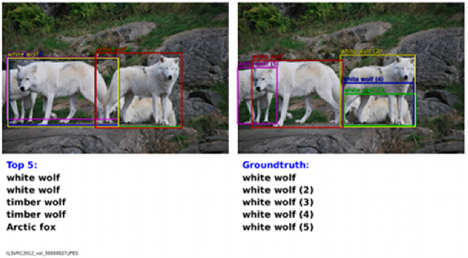
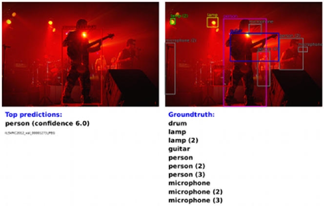
Throughout the paper, we report results on the 2013 ImageNet Large Scale Visual Recognition Challenge (ILSVRC2013). In the classification task of this challenge, each image is assigned a single label corresponding to the main object in the image. Five guesses are allowed to find the correct answer (this is because images can also contain multiple unlabeled objects). The localization task is similar in that 5 guesses are allowed per image, but in addition, a bounding box for the predicted object must be returned with each guess. To be considered correct, the predicted box must match the groundtruth by at least 50% (using the PASCAL criterion of union over intersection), as well as be labeled with the correct class (i.e. each prediction is a label and bounding box that are associated together). The detection task differs from localization in that there can be any number of objects in each image (including zero), and false positives are penalized by the mean average precision (mAP) measure. The localization task is a convenient intermediate step between classification and detection, and allows us to evaluate our localization method independently of challenges specific to detection (such as learning a background class). In Fig. 1, we show examples of images with our localization/detection predictions as well as corresponding groundtruth. Note that classification and localization share the same dataset, while detection also has additional data where objects can be smaller. The detection data also contain a set of images where certain objects are absent. This can be used for bootstrapping, but we have not made use of it in this work.

3 Classification

Our classification architecture is similar to the best ILSVRC12 architecture by Krizhevsky et al. [15]. However, we improve on the network design and the inference step. Because of time constraints, some of the training features in Krizhevsky’s model were not explored, and so we expect our results can be improved even further. These are discussed in the future work section 6

Figure 2: Layer 1 (top) and layer 2 filters (bottom).

3.1 Model Design and Training

We train the network on the ImageNet 2012 training set (1.2 million images and $C=1000$ classes) [5]. Our model uses the same fixed input size approach proposed by Krizhevsky et al. [15] during training but turns to multi-scale for classification as described in the next section. Each image is downsampled so that the smallest dimension is 256 pixels. We then extract 5 random crops (and their horizontal flips) of size 221x221 pixels and present these to the network in mini-batches of size 128. The weights in the network are initialized randomly with $(\mu,\sigma)=(0,1\times 10^{-2})$. They are then updated by stochastic gradient descent, accompanied by momentum term of $0.6$ and an $\ell_{2}$ weight decay of $1\times 10^{-5}$. The learning rate is initially $5\times 10^{-2}$ and is successively decreased by a factor of $0.5$ after $(30,50,60,70,80)$ epochs. DropOut [11] with a rate of $0.5$ is employed on the fully connected layers (6th and 7th) in the classifier.

								Output
Layer	1	2	3	4	5	6	7	8
Stage	conv + max	conv + max	conv	conv	conv + max	full	full	full
# channels	96	256	512	1024	1024	3072	4096	1000
Filter size	11x11	5x5	3x3	3x3	3x3	-	-	-
Conv. stride	4x4	1x1	1x1	1x1	1x1	-	-	-
Pooling size	2x2	2x2	-	-	2x2	-	-	-
Pooling stride	2x2	2x2	-	-	2x2	-	-	-
Zero-Padding size	-	-	1x1x1x1	1x1x1x1	1x1x1x1	-	-	-
Spatial input size	231x231	24x24	12x12	12x12	12x12	6x6	1x1	1x1

Table 1: Architecture specifics for fast model. The spatial size of the feature maps depends on the input image size, which varies during our inference step (see Table 5 in the Appendix). Here we show training spatial sizes. Layer 5 is the top convolutional layer. Subsequent layers are fully connected, and applied in sliding window fashion at test time. The fully-connected layers can also be seen as 1x1 convolutions in a spatial setting. Similar sizes for accurate model can be found in the Appendix.

We detail the architecture sizes in tables 1 and 3. Note that during training, we treat this architecture as non-spatial (output maps of size 1x1), as opposed to the inference step, which produces spatial outputs. Layers 1-5 are similar to Krizhevsky et al. [15], using rectification (“relu”) non-linearities and max pooling, but with the following differences: (i) no contrast normalization is used; (ii) pooling regions are non-overlapping and (iii) our model has larger 1st and 2nd layer feature maps, thanks to a smaller stride (2 instead of 4). A larger stride is beneficial for speed but will hurt accuracy.

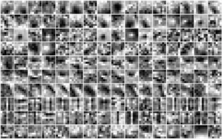
In Fig. 2, we show the filter coefficients from the first two convolutional layers. The first layer filters capture orientated edges, patterns and blobs. In the second layer, the filters have a variety of forms, some diffuse, others with strong line structures or oriented edges.

3.2 Feature Extractor

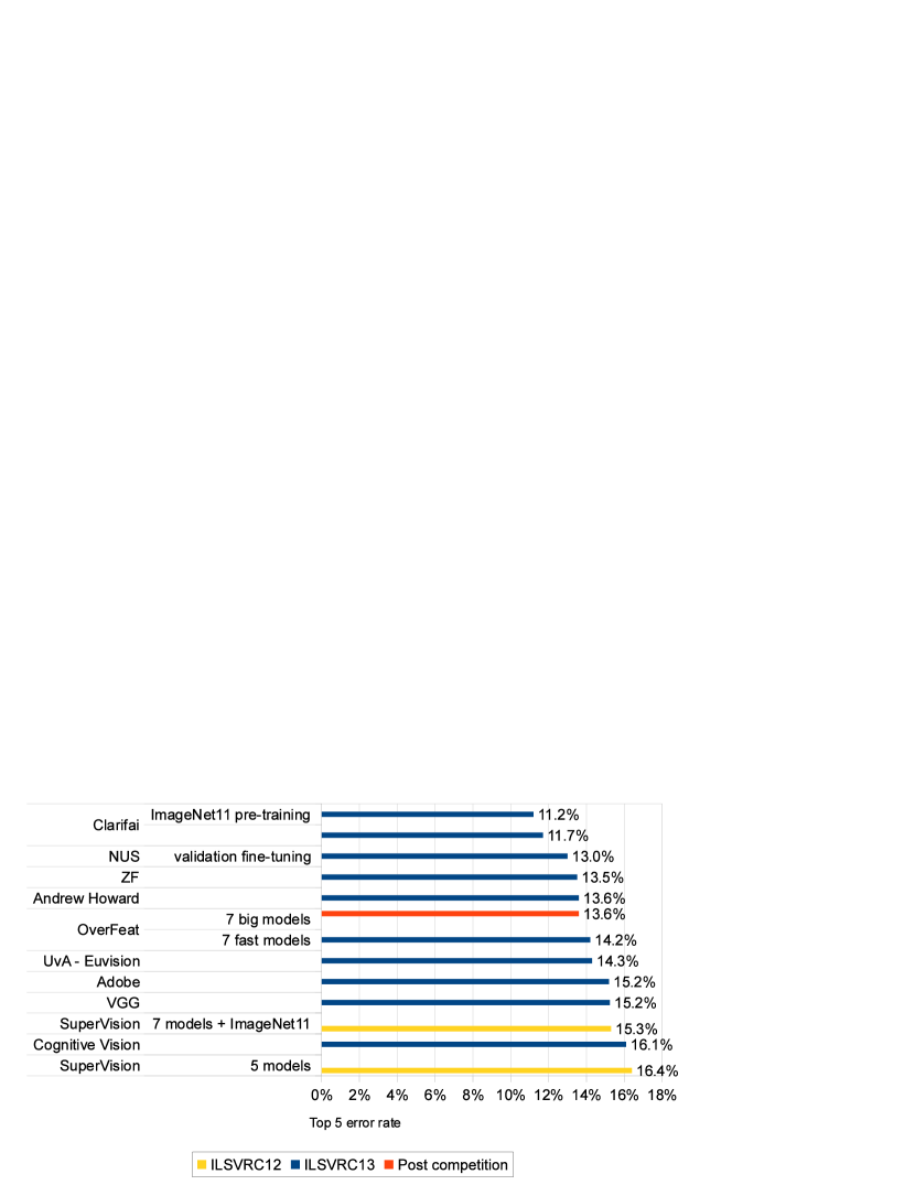
Along with this paper, we release a feature extractor named “OverFeat”  in order to provide powerful features for computer vision research. Two models are provided, a fast and accurate one. Each architecture is described in tables 1 and 3. We also compare their sizes in Table 4 in terms of parameters and connections. The accurate model is more accurate than the fast one (14.18% classification error as opposed to 16.39% in Table 2), however it requires nearly twice as many connections. Using a committee of 7 accurate models reaches 13.6% classification error as shown in Fig. 4.

3.3 Multi-Scale Classification

In [15], multi-view voting is used to boost performance: a fixed set of 10 views (4 corners and center, with horizontal flip) is averaged. However, this approach can ignore many regions of the image, and is computationally redundant when views overlap. Additionally, it is only applied at a single scale, which may not be the scale at which the ConvNet will respond with optimal confidence.

Instead, we explore the entire image by densely running the network at each location and at multiple scales. While the sliding window approach may be computationally prohibitive for certain types of model, it is inherently efficient in the case of ConvNets (see section 3.5). This approach yields significantly more views for voting, which increases robustness while remaining efficient. The result of convolving a ConvNet on an image of arbitrary size is a spatial map of $C$-dimensional vectors at each scale.

However, the total subsampling ratio in the network described above is 2x3x2x3, or 36. Hence when applied densely, this architecture can only produce a classification vector every 36 pixels in the input dimension along each axis. This coarse distribution of outputs decreases performance compared to the 10-view scheme because the network windows are not well aligned with the objects in the images. The better aligned the network window and the object, the strongest the confidence of the network response. To circumvent this problem, we take an approach similar to that introduced by Giusti et al. [9], and apply the last subsampling operation at every offset. This removes the loss of resolution from this layer, yielding a total subsampling ratio of x12 instead of x36.

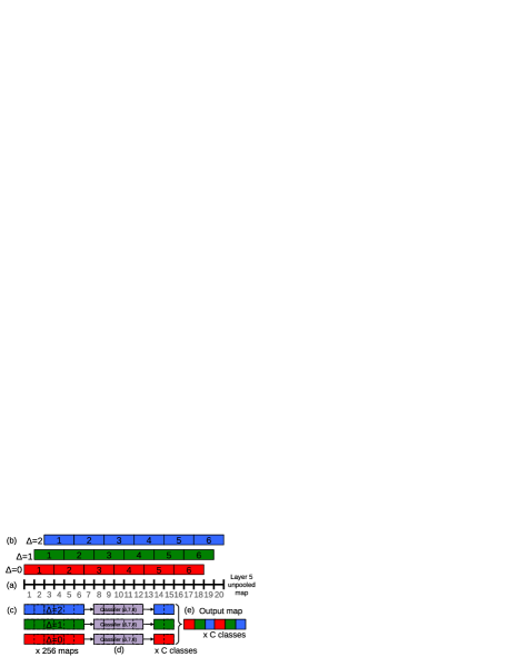
We now explain in detail how the resolution augmentation is performed. We use 6 scales of input which result in unpooled layer 5 maps of varying resolution (see Table 5 for details). These are then pooled and presented to the classifier using the following procedure, illustrated in Fig. 3:

1. For a single image, at a given scale, we start with the unpooled layer 5 feature maps.

2. Each of unpooled maps undergoes a 3x3 max pooling operation (non-overlapping regions), repeated 3x3 times for $(\Delta_{x},\Delta_{y})$ pixel offsets of $\{0,1,2\}$.

3. This produces a set of pooled feature maps, replicated (3x3) times for different $(\Delta_{x},\Delta_{y})$ combinations.

4. The classifier (layers 6,7,8) has a fixed input size of 5x5 and produces a $C$-dimensional output vector for each location within the pooled maps. The classifier is applied in sliding-window fashion to the pooled maps, yielding $C$-dimensional output maps (for a given $(\Delta_{x},\Delta_{y})$ combination).

5. The output maps for different $(\Delta_{x},\Delta_{y})$ combinations are reshaped into a single 3D output map (two spatial dimensions x $C$ classes).

Figure 3: 1D illustration (to scale) of output map computation for classification, using $y$-dimension from scale 2 as an example (see Table 5). (a): 20 pixel unpooled layer 5 feature map. (b): max pooling over non-overlapping 3 pixel groups, using offsets of $\Delta=\{0,1,2\}$ pixels (red, green, blue respectively). (c): The resulting 6 pixel pooled maps, for different $\Delta$. (d): 5 pixel classifier (layers 6,7) is applied in sliding window fashion to pooled maps, yielding 2 pixel by $C$ maps for each $\Delta$. (e): reshaped into 6 pixel by $C$ output maps.

These operations can be viewed as shifting the classifier’s viewing window by 1 pixel through pooling layers without subsampling and using skip-kernels in the following layer (where values in the neighborhood are non-adjacent). Or equivalently, as applying the final pooling layer and fully-connected stack at every possible offset, and assembling the results by interleaving the outputs.

The procedure above is repeated for the horizontally flipped version of each image. We then produce the final classification by (i) taking the spatial max for each class, at each scale and flip; (ii) averaging the resulting $C$-dimensional vectors from different scales and flips and (iii) taking the top-1 or top-5 elements (depending on the evaluation criterion) from the mean class vector.

At an intuitive level, the two halves of the network — i.e. feature extraction layers (1-5) and classifier layers (6-output) — are used in opposite ways. In the feature extraction portion, the filters are convolved across the entire image in one pass. From a computational perspective, this is far more efficient than sliding a fixed-size feature extractor over the image and then aggregating the results from different locations. However, these principles are reversed for the classifier portion of the network. Here, we want to hunt for a fixed-size representation in the layer 5 feature maps across different positions and scales. Thus the classifier has a fixed-size 5x5 input and is exhaustively applied to the layer 5 maps. The exhaustive pooling scheme (with single pixel shifts $(\Delta_{x},\Delta_{y})$) ensures that we can obtain fine alignment between the classifier and the representation of the object in the feature map.

3.4 Results

In Table 2, we experiment with different approaches, and compare them to the single network model of Krizhevsky et al. [15] for reference. The approach described above, with 6 scales, achieves a top-5 error rate of 13.6%. As might be expected, using fewer scales hurts performance: the single-scale model is worse with 16.97% top-5 error. The fine stride technique illustrated in Fig. 3 brings a relatively small improvement in the single scale regime, but is also of importance for the multi-scale gains shown here.

	Top-1	Top-5
Approach	error %	error %
Krizhevsky et al. [15]	40.7	18.2
OverFeat - 1 fast model, scale 1, coarse stride	39.28	17.12
OverFeat - 1 fast model, scale 1, fine stride	39.01	16.97
OverFeat - 1 fast model, 4 scales (1,2,4,6), fine stride	38.57	16.39
OverFeat - 1 fast model, 6 scales (1-6), fine stride	38.12	16.27
OverFeat - 1 accurate model, 4 corners + center + flip	35.60	14.71
OverFeat - 1 accurate model, 4 scales, fine stride	35.74	14.18
OverFeat - 7 fast models, 4 scales, fine stride	35.10	13.86
OverFeat - 7 accurate models, 4 scales, fine stride	33.96	13.24

Table 2: Classification experiments on validation set. Fine/coarse stride refers to the number of $\Delta$ values used when applying the classifier. Fine: $\Delta={0,1,2}$; coarse: $\Delta=0$.

We report the test set results of the 2013 competition in Fig. 4 where our model (OverFeat) obtained 14.2% accuracy by voting of 7 ConvNets (each trained with different initializations) and ranked 5th out of 18 teams. The best accuracy using only ILSVRC13 data was 11.7%. Pre-training with extra data from the ImageNet Fall11 dataset improved this number to 11.2%. In post-competition work, we improve the OverFeat results down to 13.6% error by using bigger models (more features and more layers). Due to time constraints, these bigger models are not fully trained, more improvements are expected to appear in time.

Figure 4: Test set classification results. During the competition, OverFeat yielded 14.2% top 5 error rate using an average of 7 fast models. In post-competition work, OverFeat ranks fifth with 13.6% error using bigger models (more features and more layers).

3.5 ConvNets and Sliding Window Efficiency

In contrast to many sliding-window approaches that compute an entire pipeline for each window of the input one at a time, ConvNets are inherently efficient when applied in a sliding fashion because they naturally share computations common to overlapping regions. When applying our network to larger images at test time, we simply apply each convolution over the extent of the full image. This extends the output of each layer to cover the new image size, eventually producing a map of output class predictions, with one spatial location for each “window” (field of view) of input. This is diagrammed in Fig. 5. Convolutions are applied bottom-up, so that the computations common to neighboring windows need only be done once.

Note that the last layers of our architecture are fully connected linear layers. At test time, these layers are effectively replaced by convolution operations with kernels of 1x1 spatial extent. The entire ConvNet is then simply a sequence of convolutions, max-pooling and thresholding operations exclusively.

Figure 5: The efficiency of ConvNets for detection. During training, a ConvNet produces only a single spatial output (top). But when applied at test time over a larger image, it produces a spatial output map, e.g. 2x2 (bottom). Since all layers are applied convolutionally, the extra computation required for the larger image is limited to the yellow regions. This diagram omits the feature dimension for simplicity.

4 Localization

Starting from our classification-trained network, we replace the classifier layers by a regression network and train it to predict object bounding boxes at each spatial location and scale. We then combine the regression predictions together, along with the classification results at each location, as we now describe.

4.1 Generating Predictions

To generate object bounding box predictions, we simultaneously run the classifier and regressor networks across all locations and scales. Since these share the same feature extraction layers, only the final regression layers need to be recomputed after computing the classification network. The output of the final softmax layer for a class $c$ at each location provides a score of confidence that an object of class $c$ is present (though not necessarily fully contained) in the corresponding field of view. Thus we can assign a confidence to each bounding box.

Figure 6: Localization/Detection pipeline. The raw classifier/detector outputs a class and a confidence for each location (1st diagram). The resolution of these predictions can be increased using the method described in section 3.3 (2nd diagram). The regression then predicts the location scale of the object with respect to each window (3rd diagram). These bounding boxes are then merge and accumulated to a small number of objects (4th diagram).

Figure 7: Examples of bounding boxes produced by the regression network, before being combined into final predictions. The examples shown here are at a single scale. Predictions may be more optimal at other scales depending on the objects. Here, most of the bounding boxes which are initially organized as a grid, converge to a single location and scale. This indicates that the network is very confident in the location of the object, as opposed to being spread out randomly. The top left image shows that it can also correctly identify multiple location if several objects are present. The various aspect ratios of the predicted bounding boxes shows that the network is able to cope with various object poses.

4.2 Regressor Training

The regression network takes as input the pooled feature maps from layer 5. It has 2 fully-connected hidden layers of size 4096 and 1024 channels, respectively. The final output layer has 4 units which specify the coordinates for the bounding box edges. As with classification, there are (3x3) copies throughout, resulting from the $\Delta_{x},\Delta_{y}$ shifts. The architecture is shown in Fig. 8.

Figure 8: Application of the regression network to layer 5 features, at scale 2, for example. (a) The input to the regressor at this scale are 6x7 pixels spatially by 256 channels for each of the (3x3) $\Delta_{x},\Delta_{y}$ shifts. (b) Each unit in the 1st layer of the regression net is connected to a 5x5 spatial neighborhood in the layer 5 maps, as well as all 256 channels. Shifting the 5x5 neighborhood around results in a map of 2x3 spatial extent, for each of the 4096 channels in the layer, and for each of the (3x3) $\Delta_{x},\Delta_{y}$ shifts. (c) The 2nd regression layer has 1024 units and is fully connected (i.e. the purple element only connects to the purple element in (b), across all 4096 channels). (d) The output of the regression network is a 4-vector (specifying the edges of the bounding box) for each location in the 2x3 map, and for each of the (3x3) $\Delta_{x},\Delta_{y}$ shifts.

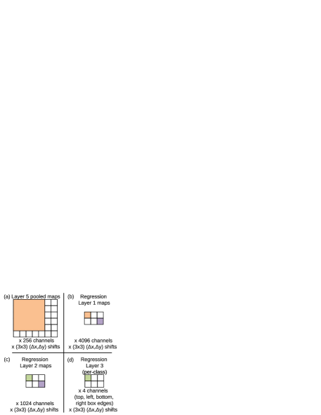
We fix the feature extraction layers (1-5) from the classification network and train the regression network using an $\ell_{2}$ loss between the predicted and true bounding box for each example. The final regressor layer is class-specific, having 1000 different versions, one for each class. We train this network using the same set of scales as described in Section 3. We compare the prediction of the regressor net at each spatial location with the ground-truth bounding box, shifted into the frame of reference of the regressor’s translation offset within the convolution (see Fig. 8). However, we do not train the regressor on bounding boxes with less than 50% overlap with the input field of view: since the object is mostly outside of these locations, it will be better handled by regression windows that do contain the object.

Training the regressors in a multi-scale manner is important for the across-scale prediction combination. Training on a single scale will perform well on that scale and still perform reasonably on other scales. However training multi-scale will make predictions match correctly across scales and exponentially increase the confidence of the merged predictions. In turn, this allows us to perform well with a few scales only, rather than many scales as is typically the case in detection. The typical ratio from one scale to another in pedestrian detection [25] is about 1.05 to 1.1, here however we use a large ratio of approximately 1.4 (this number differs for each scale since dimensions are adjusted to fit exactly the stride of our network) which allows us to run our system faster.

4.3 Combining Predictions

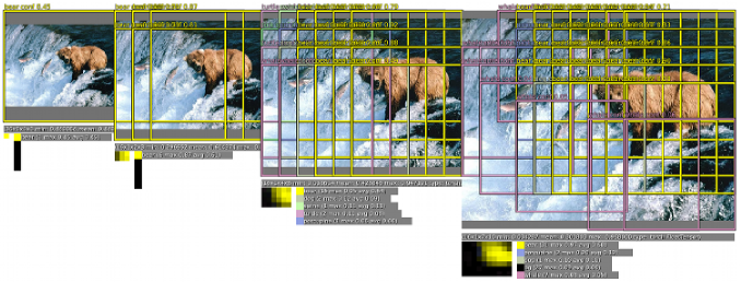
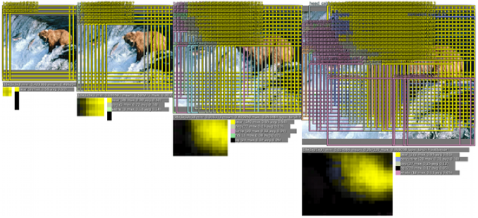
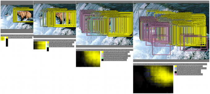
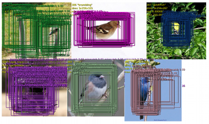
We combine the individual predictions (see Fig. 7) via a greedy merge strategy applied to the regressor bounding boxes, using the following algorithm.

1. Assign to $C_{s}$ the set of classes in the top $k$ for each scale $s\in 1\dots 6$, found by taking the maximum detection class outputs across spatial locations for that scale.

2. Assign to $B_{s}$ the set of bounding boxes predicted by the regressor network for each class in $C_{s}$, across all spatial locations at scale $s$.

3. Assign $B\leftarrow\bigcup_{s}B_{s}$

4. Repeat merging until done:

5. $(b_{1}^{*},b_{2}^{*})={\rm argmin}_{b_{1}\neq b_{2}\in B}{\tt match\_score(b_{1},b_{2})}$

6. If ${\tt match\_score}(b_{1}^{*},b_{2}^{*})>t$ , stop.

7. Otherwise, set $B\leftarrow B\backslash\{b_{1}^{*},b_{2}^{*}\}\cup{\tt box\_merge}(b_{1}^{*},b_{2}^{*})$

In the above, we compute match_score using the sum of the distance between centers of the two bounding boxes and the intersection area of the boxes. box_merge compute the average of the bounding boxes’ coordinates.

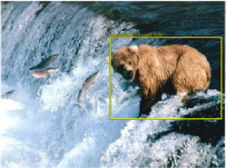
The final prediction is given by taking the merged bounding boxes with maximum class scores. This is computed by cumulatively adding the detection class outputs associated with the input windows from which each bounding box was predicted. See Fig. 6 for an example of bounding boxes merged into a single high-confidence bounding box. In that example, some turtle and whale bounding boxes appear in the intermediate multi-scale steps, but disappear in the final detection image. Not only do these bounding boxes have low classification confidence (at most 0.11 and 0.12 respectively), their collection is not as coherent as the bear bounding boxes to get a significant confidence boost. The bear boxes have a strong confidence (approximately 0.5 on average per scale) and high matching scores. Hence after merging, many bear bounding boxes are fused into a single very high confidence box, while false positives disappear below the detection threshold due their lack of bounding box coherence and confidence. This analysis suggest that our approach is naturally more robust to false positives coming from the pure-classification model than traditional non-maximum suppression, by rewarding bounding box coherence.

4.4 Experiments

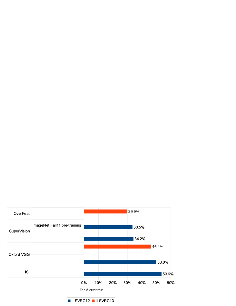
We apply our network to the Imagenet 2012 validation set using the localization criterion specified for the competition. The results for this are shown in Fig. 9. Fig. 10 shows the results of the 2012 and 2013 localization competitions (the train and test data are the same for both of these years). Our method is the winner of the 2013 competition with 29.9% error.

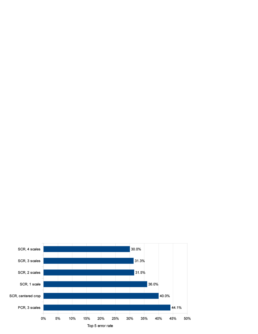
Our multiscale and multi-view approach was critical to obtaining good performance, as can be seen in Fig. 9: Using only a single centered crop, our regressor network achieves an error rate of 40%. By combining regressor predictions from all spatial locations at two scales, we achieve a vastly better error rate of 31.5%. Adding a third and fourth scale further improves performance to 30.0% error.

Using a different top layer for each class in the regressor network for each class (Per-Class Regressor (PCR) in Fig. 9) surprisingly did not outperform using only a single network shared among all classes (44.1% vs. 31.3%). This may be because there are relatively few examples per class annotated with bounding boxes in the training set, while the network has 1000 times more top-layer parameters, resulting in insufficient training. It is possible this approach may be improved by sharing parameters only among similar classes (e.g. training one network for all classes of dogs, another for vehicles, etc.).

Figure 9: Localization experiments on ILSVRC12 validation set. We experiment with different number of scales and with the use of single-class regression (SCR) or per-class regression (PCR).

Figure 10: ILSVRC12 and ILSVRC13 competitions results (test set). Our entry is the winner of the ILSVRC13 localization competition with 29.9% error (top 5). Note that training and testing data is the same for both years. The OverFeat entry uses 4 scales and a single-class regression approach.

5 Detection

Detection training is similar to classification training but in a spatial manner. Multiple location of an image may be trained simultaneously. Since the model is convolutional, all weights are shared among all locations. The main difference with the localization task, is the necessity to predict a background class when no object is present. Traditionally, negative examples are initially taken at random for training. Then the most offending negative errors are added to the training set in bootstrapping passes. Independent bootstrapping passes render training complicated and risk potential mismatches between the negative examples collection and training times. Additionally, the size of bootstrapping passes needs to be tuned to make sure training does not overfit on a small set. To circumvent all these problems, we perform negative training on the fly, by selecting a few interesting negative examples per image such as random ones or most offending ones. This approach is more computationally expensive, but renders the procedure much simpler. And since the feature extraction is initially trained with the classification task, the detection fine-tuning is not as long anyway.

Figure 11: ILSVRC13 test set Detection results. During the competition, UvA ranked first with 22.6% mAP. In post competition work, we establish a new state of the art with 24.3% mAP. Systems marked with * were pre-trained with the ILSVRC12 classification data.

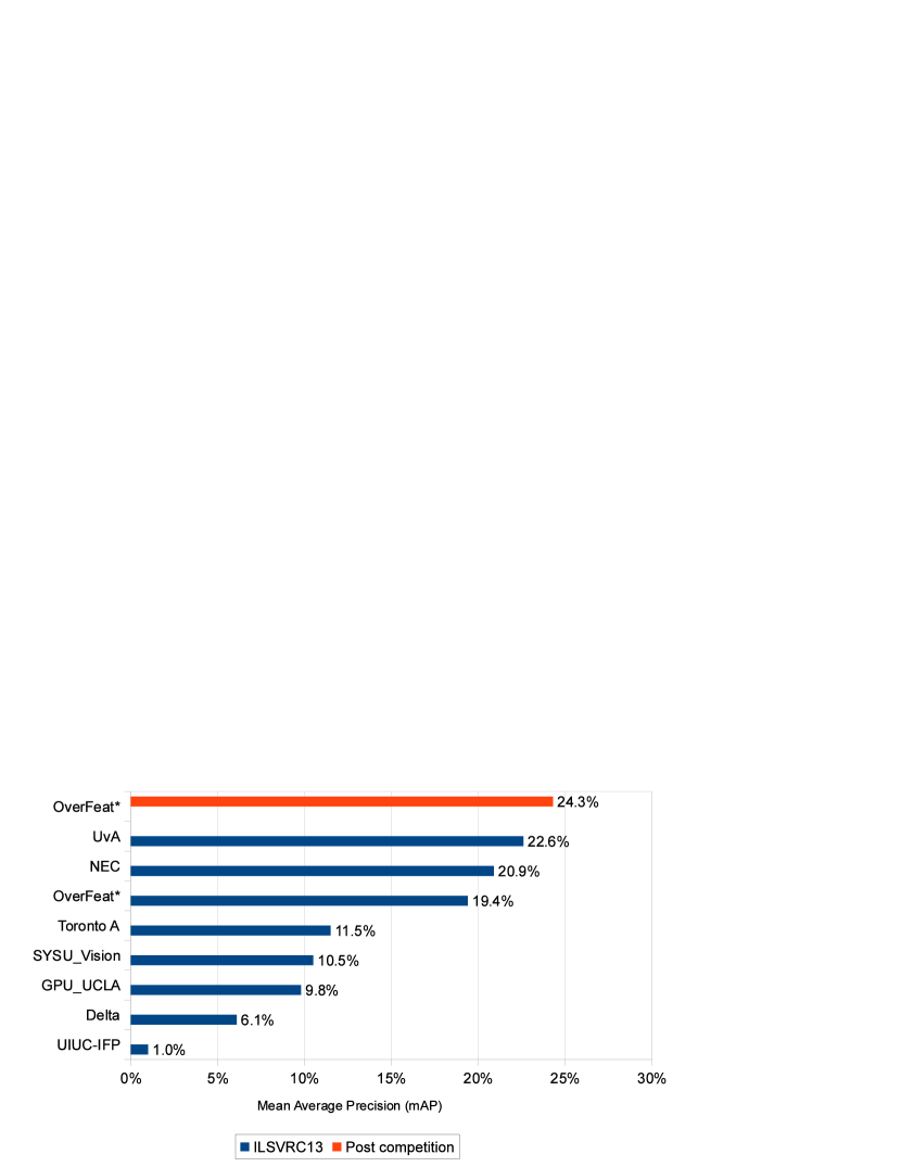
In Fig. 11, we report the results of the ILSVRC 2013 competition where our detection system ranked 3rd with 19.4% mean average precision (mAP). We later established a new detection state of the art with 24.3% mAP. Note that there is a large gap between the top 3 methods and other teams (the 4th method yields 11.5% mAP). Additionally, our approach is considerably different from the top 2 other systems which use an initial segmentation step to reduce candidate windows from approximately 200,000 to 2,000. This technique speeds up inference and substantially reduces the number of potential false positives. [29, 1] suggest that detection accuracy drops when using dense sliding window as opposed to selective search which discards unlikely object locations hence reducing false positives. Combined with our method, we may observe similar improvements as seen here between traditional dense methods and segmentation based methods. It should also be noted that we did not fine tune on the detection validation set as NEC and UvA did. The validation and test set distributions differ significantly enough from the training set that this alone improves results by approximately 1 point. The improvement between the two OverFeat results in Fig. 11 are due to longer training times and the use of context, i.e. each scale also uses lower resolution scales as input.

6 Discussion

We have presented a multi-scale, sliding window approach that can be used for classification, localization and detection. We applied it to the ILSVRC 2013 datasets, and it currently ranks 4^th in classification, 1^st in localization and 1^st in detection. A second important contribution of our paper is explaining how ConvNets can be effectively used for detection and localization tasks. These were never addressed in [15] and thus we are the first to explain how this can be done in the context of ImageNet 2012. The scheme we propose involves substantial modifications to networks designed for classification, but clearly demonstrate that ConvNets are capable of these more challenging tasks. Our localization approach won the 2013 ILSVRC competition and significantly outperformed all 2012 and 2013 approaches. The detection model was among the top performers during the competition, and ranks first in post-competition results. We have proposed an integrated pipeline that can perform different tasks while sharing a common feature extraction base, entirely learned directly from the pixels.

Our approach might still be improved in several ways. (i) For localization, we are not currently back-propping through the whole network; doing so is likely to improve performance. (ii) We are using $\ell_{2}$ loss, rather than directly optimizing the intersection-over-union (IOU) criterion on which performance is measured. Swapping the loss to this should be possible since IOU is still differentiable, provided there is some overlap. (iii) Alternate parameterizations of the bounding box may help to decorrelate the outputs, which will aid network training.

Appendix: Additional Model Details

									Output
Layer	1	2	3	4	5	6	7	8	9
Stage	conv + max	conv + max	conv	conv	conv	conv + max	full	full	full
# channels	96	256	512	512	1024	1024	4096	4096	1000
Filter size	7x7	7x7	3x3	3x3	3x3	3x3	-	-	-
Conv. stride	2x2	1x1	1x1	1x1	1x1	1x1	-	-	-
Pooling size	3x3	2x2	-	-	-	3x3	-	-	-
Pooling stride	3x3	2x2	-	-	-	3x3	-	-	-
Zero-Padding size	-	-	1x1x1x1	1x1x1x1	1x1x1x1	1x1x1x1	-	-	-
Spatial input size	221x221	36x36	15x15	15x15	15x15	15x15	5x5	1x1	1x1

Table 3: Architecture specifics for accurate model. It differs from the fast model mainly in the stride of the first convolution, the number of stages and the number of feature maps.

model	# parameters (in millions)	# connections (in millions)
Krizhevsky	60	-
fast	145	2810
accurate	144	5369

Table 4: Number of parameters and connections for different models.

	Input	Layer 5	Layer 5	Classifier	Classifier
Scale	size	pre-pool	post-pool	map (pre-reshape)	map size
1	245x245	17x17	(5x5)x(3x3)	(1x1)x(3x3)x$C$	3x3x$C$
2	281x317	20x23	(6x7)x(3x3)	(2x3)x(3x3)x$C$	6x9x$C$
3	317x389	23x29	(7x9)x(3x3)	(3x5)x(3x3)x$C$	9x15x$C$
4	389x461	29x35	(9x11)x(3x3)	(5x7)x(3x3)x$C$	15x21x$C$
5	425x497	32x35	(10x11)x(3x3)	(6x7)x(3x3)x$C$	18x24x$C$
6	461x569	35x44	(11x14)x(3x3)	(7x10)x(3x3)x$C$	21x30x$C$

Table 5: Spatial dimensions of our multi-scale approach. 6 different sizes of input images are used, resulting in layer 5 unpooled feature maps of differing spatial resolution (although not indicated in the table, all have 256 feature channels). The (3x3) results from our dense pooling operation with $(\Delta_{x},\Delta_{y})=\{0,1,2\}$. See text and Fig. 3 for details for how these are converted into output maps.

References

- [1] J. Carreira, F. Li, and C. Sminchisescu. Object recognition by sequential figure-ground ranking. International journal of computer vision, 98(3):243–262, 2012.
- [2] J. Carreira and C. Sminchisescu. Constrained parametric min-cuts for automatic object segmentation, release 1. http://sminchisescu.ins.uni-bonn.de/code/cpmc/.
- [3] D. C. Ciresan, J. Meier, and J. Schmidhuber. Multi-column deep neural networks for image classification. In CVPR, 2012.
- [4] M. Delakis and C. Garcia. Text detection with convolutional neural networks. In International Conference on Computer Vision Theory and Applications (VISAPP 2008), 2008.
- [5] J. Deng, W. Dong, R. Socher, L.-J. Li, K. Li, and L. Fei-Fei. ImageNet: A Large-Scale Hierarchical Image Database. In CVPR09, 2009.
- [6] I. Endres and D. Hoiem. Category independent object proposals. In Computer Vision–ECCV 2010, pages 575–588. Springer, 2010.
- [7] C. Farabet, C. Couprie, L. Najman, and Y. LeCun. Learning hierarchical features for scene labeling. IEEE Transactions on Pattern Analysis and Machine Intelligence, 2013. in press.
- [8] C. Garcia and M. Delakis. Convolutional face finder: A neural architecture for fast and robust face detection. IEEE Transactions on Pattern Analysis and Machine Intelligence, 2004.
- [9] A. Giusti, D. C. Ciresan, J. Masci, L. M. Gambardella, and J. Schmidhuber. Fast image scanning with deep max-pooling convolutional neural networks. In International Conference on Image Processing (ICIP), 2013.
- [10] R. Hadsell, P. Sermanet, M. Scoffier, A. Erkan, K. Kavackuoglu, U. Muller, and Y. LeCun. Learning long-range vision for autonomous off-road driving. Journal of Field Robotics, 26(2):120–144, February 2009.
- [11] G. Hinton, N. Srivastave, A. Krizhevsky, I. Sutskever, and R. R. Salakhutdinov. Improving neural networks by preventing co-adaptation of feature detectors. arXiv:1207.0580, 2012.
- [12] G. E. Hinton, A. Krizhevsky, and S. D. Wang. Transforming auto-encoders. In Artificial Neural Networks and Machine Learning–ICANN 2011, pages 44–51. Springer Berlin Heidelberg, 2011.
- [13] V. Jain, J. F. Murray, F. Roth, S. Turaga, V. Zhigulin, K. Briggman, M. Helmstaedter, W. Denk, and H. S. Seung. Supervised learning of image restoration with convolutional networks. In ICCV’07.
- [14] K. Jarrett, K. Kavukcuoglu, M. Ranzato, and Y. LeCun. What is the best multi-stage architecture for object recognition? In Proc. International Conference on Computer Vision (ICCV’09). IEEE, 2009.
- [15] A. Krizhevsky, I. Sutskever, and G. Hinton. Imagenet classification with deep convolutional neural networks. In NIPS, 2012.
- [16] Y. LeCun, B. Boser, J. S. Denker, D. Henderson, R. E. Howard, W. Hubbard, and L. D. Jackel. Handwritten digit recognition with a back-propagation network. In D. Touretzky, editor, Advances in Neural Information Processing Systems (NIPS 1989), volume 2, Denver, CO, 1990. Morgan Kaufman.
- [17] Y. LeCun, L. Bottou, Y. Bengio, and P. Haffner. Gradient-based learning applied to document recognition. Proceedings of the IEEE, 86(11):2278–2324, November 1998.
- [18] Y. LeCun, F.-J. Huang, and L. Bottou. Learning methods for generic object recognition with invariance to pose and lighting. In Proceedings of CVPR’04. IEEE Press, 2004.
- [19] S. Manen, M. Guillaumin, and L. Van Gool. Prime object proposals with randomized prim’s algorithm. In International Conference on Computer Vision (ICCV), 2013.
- [20] O. Matan, J. Bromley, C. Burges, J. Denker, L. Jackel, Y. LeCun, E. Pednault, W. Satterfield, C. Stenard, and T. Thompson. Reading handwritten digits: A zip code recognition system. IEEE Computer, 25(7):59–63, July 1992.
- [21] F. Ning, D. Delhomme, Y. LeCun, F. Piano, L. Bottou, and P. Barbano. Toward automatic phenotyping of developing embryos from videos. IEEE Transactions on Image Processing, 14(9):1360–1371, September 2005. Special issue on Molecular and Cellular Bioimaging.
- [22] S. Nowlan and J. Platt. A convolutional neural network hand tracker. pages 901–908, San Mateo, CA, 1995. Morgan Kaufmann.
- [23] M. Osadchy, Y. LeCun, and M. Miller. Synergistic face detection and pose estimation with energy-based models. Journal of Machine Learning Research, 8:1197–1215, May 2007.
- [24] P. Sermanet, S. Chintala, and Y. LeCun. Convolutional neural networks applied to house numbers digit classification. In International Conference on Pattern Recognition (ICPR 2012), 2012.
- [25] P. Sermanet, K. Kavukcuoglu, S. Chintala, and Y. LeCun. Pedestrian detection with unsupervised multi-stage feature learning. In Proc. International Conference on Computer Vision and Pattern Recognition (CVPR’13). IEEE, June 2013.
- [26] P. Sermanet and Y. LeCun. Traffic sign recognition with multi-scale convolutional networks. In Proceedings of International Joint Conference on Neural Networks (IJCNN’11), 2011.
- [27] G. Taylor, R. Fergus, G. Williams, I. Spiro, and C. Bregler. Pose-sensitive embedding by nonlinear nca regression. In NIPS, 2011.
- [28] G. Taylor, I. Spiro, C. Bregler, and R. Fergus. Learning invarance through imitation. In CVPR, 2011.
- [29] J. R. R. Uijlings, K. E. A. van de Sande, T. Gevers, and A. W. M. Smeulders. Selective search for object recognition. International Journal of Computer Vision, 104(2):154–171, 2013.
- [30] R. Vaillant, C. Monrocq, and Y. LeCun. Original approach for the localisation of objects in images. IEE Proc on Vision, Image, and Signal Processing, 141(4):245–250, August 1994.