The Cauchy-Schwarz divergence for Poisson point processes

Abstract

In this paper, we extend the notion of Cauchy-Schwarz divergence to point processes and establish that the Cauchy-Schwarz divergence between the probability densities of two Poisson point processes is half the squared ${L^{2}}$-distance between their intensity functions. Extension of this result to mixtures of Poisson point processes and, in the case where the intensity functions are Gaussian mixtures, closed form expressions for the Cauchy-Schwarz divergence are presented. Our result also implies that the Bhattacharyya distance between the probability distributions of two Poisson point processes is equal to the square of the Hellinger distance between their intensity measures. We illustrate the result via a sensor management application where the system states are modeled as point processes.

I Introduction

The Poisson point process, which models “no interaction” or “complete spatial randomness” in spatial point patterns, is arguably one of the best known and most tractable of point processes [2, 3, 4, 5, 6]. Point process theory is the study of random counting measures with applications spanning numerous disciplines, see for example [2, 3, 6, 7, 8]. The Poisson point process itself arises in forestry [9], geology [10], biology [11], particle physics [12], communication networks [13, 14, 15] and signal processing [16, 17, 18]. The role of the Poisson point process in point process theory, in most respects, is analogous to that of the normal distribution in random vectors [19].

Similarity measures between random variables are fundamental in information theory and statistical analysis [20]. Information theoretic divergences, for example Kullback-Leibler, Rényi (or $\alpha$-divergence) and their generalization Csiszár-Morimoto (or Ali-Silvey), Jensen-Rényi, Cauchy-Schwarz etc., measure the difference between the information content of the random variables. Similarity between random variables can also be measured via the statistical distance between their probability distributions, for example total variation, Bhattacharyya, Hellinger/Matusita, Wasserstein, etc. Some distances are actually special cases of $f$-divergences [21]. Note that statistical distances are not necessarily proper metrics.

For point processes or random finite sets, similarity measures have been studied extensively in various application areas such as sensor management [22, 23, 24, 25, 26, 27] and neuroscience [28]. However, so far except for trivial special cases, these similarity measures cannot be computed analytically and require expensive approximations such as Monte Carlo.

In this paper, we present results on similarity measures for Poisson point processes via the Cauchy-Schwarz divergence and its relationship to the Bhattacharyya and Hellinger distances. In particular, we show that the Cauchy-Schwarz divergence between two Poisson point processes is given by the square of the $L^{2}$-distance between their intensity functions. Geometrically, this result relates the angle subtended by the probability densities of the Poisson point processes to the $L^{2}$-distance between their corresponding intensity functions. For Gaussian mixture intensity functions, their $L^{2}$-distance, and hence the Cauchy-Schwarz divergence can be evaluated analytically. We also extend the result to the Cauchy-Schwarz divergence for mixtures of Poisson point processes. In addition, using our result on the Cauchy-Schwarz divergence, we show that the Bhattacharyya distance between the probability distributions of two Poisson point processes is the square of the Hellinger distance between their respective intensity measures. The Poisson point process enjoys a number of nice properties [2, 3, 4], and our results are useful additions. We illustrate the use of our result on the Cauchy-Schwarz divergence in a sensor management application for multi-target tracking involving the Probability Hypothesis Density (PHD) filter [16].

The organization of the paper is as follows. Background on point processes and the Cauchy-Schwarz divergence is provided in Section II. Section III presents the main results of the paper that establish the analytical formulation for the Cauchy-Schwarz divergence and Bhattacharyya distance between two Poisson point processes. In Section IV, the application of the Cauchy-Schwarz divergence to sensor management, including numerical examples, is studied. Finally, Section V concludes the paper.

II Background

In this work we consider a state space $\mathcal{X}\subseteq\mathbb{R}^{d}$, and adopt the inner product notation $\left\langle f,g\right\rangle\triangleq\int f(x)g(x)dx$; the $L^{2}$-norm notation $\left\|f\right\|\triangleq\sqrt{\left\langle f,f\right\rangle}$; the multi-target exponential notation $h^{X}\triangleq\prod_{x\in X}h(x)$, where $h$ is a real-valued function, with $h^{\emptyset}=1$ by convention; and the indicator function notation

$$1_{B}(x)\triangleq\left\{\begin{array}[]{l}1,\text{ if }x\in B\\ 0,\text{ otherwise}\end{array}\right..$$

The notation $\mathcal{N}(x;m,Q)$ is used to explicitly denote the probability density of a Gaussian random variable with mean $m$ and covariance $Q$, evaluated at $x$.

II-A Point processes

This section briefly summarizes concepts in point process theory needed for the exposition of our result. Point process theory, in general, is concerned with random counting measures. Our result is restricted to simple-finite point processes, which can be regarded as random finite sets. For simplicity, we omit the prefix “simple-finite” in the rest of the paper. For an introduction to the subject we refer the reader to the article [7], and for detailed treatments, books such as [2, 3, 5, 6].

A point process or random finite set $X$ on $\mathcal{X}$ is a random variable taking values in $\mathcal{F}(\mathcal{X})$, the space of finite subsets of $\mathcal{X}$. Let $|X|$ denotes the number of elements in a set $X$. A point process $X$ on $\mathcal{X}$ is said to be Poisson with a given intensity function $u$ (defined on $\mathcal{X}$) if [2, 3]:

1. for any $B\subseteq\mathcal{X}$ such that $\left\langle u,1_{B}\right\rangle<\infty$, the random variable $|X\cap B|$ is Poisson distributed with mean $\left\langle u,1_{B}\right\rangle$,

2. for any disjoint $B_{1},...,B_{i}\subseteq\mathcal{X}$, the random variables $|X\cap B_{1}|,...,|X\cap B_{i}|$ are independent.

Since $\left\langle u,1_{B}\right\rangle$ is the expected number of points of $X$ in the region $B$, the intensity value $u(x)$ can be interpreted as the instantaneous expected number of points per unit hyper-volume at $x$. Consequently, $u(x)$ is not dimensionless in general. If hyper-volume (on $\mathcal{X}$) is measured in units of $K$ (e.g. $m^{d}$, $cm^{d}$, in^d, etc.) then the intensity function $u$ has unit $K^{-1}$.

The number of points of a Poisson point process $X$ is Poisson distributed with mean $\left\langle u,1\right\rangle$, and conditional on the number of points the elements $x$ of $X$, are independently and identically distributed (i.i.d.) according to the probability density $u(\cdot)/\left\langle u,1\right\rangle$ [2, 3, 5, 6]. It is implicit that $\left\langle u,1\right\rangle$ is finite since we only consider simple-finite point processes.

The probability distribution of a Poisson point process $X$ with intensity function $u$ is given by [6, pp. 15]

$$\!\!\!\Pr(X\in\mathcal{T})=\\ \sum_{i=0}^{\infty}\!\frac{e^{-\left\langle u,1\right\rangle}}{i{!}}\!\int_{\mathcal{X}^{i}}\!1_{\mathcal{T}}(\{x_{1},...,x_{i}\})u^{\{x_{1},...,x_{i}\}}d(x_{1},...,x_{i}),$$ (1)

for any (measurable) subset $\mathcal{T}$ of $\mathcal{F}(\mathcal{X})$, where $\mathcal{X}^{i}$ denotes the $i^{\text{th}}$-fold Cartesian product of $\mathcal{X}$, with the convention $\mathcal{X}^{0}=\{\emptyset\}$, and the integral over $\mathcal{X}^{0}$ is $1_{\mathcal{T}}(\emptyset)$. A Poisson point process is completely characterized by its intensity function (or more generally the intensity measure).

Probability densities of point processes considered in this work are defined with respect to the reference measure $\mu$ given by

$$\mu(\mathcal{T})=\sum_{i=0}^{\infty}\frac{1}{i{!K}^{i}}\int_{\mathcal{X}^{i}}1_{\mathcal{T}}(\{x_{1},...,x_{i}\})d(x_{1},...,x_{i})$$ (2)

for any (measurable) subset $\mathcal{T}$ of $\mathcal{F}(\mathcal{X})$. The measure $\mu$ is analogous to the Lebesque measure on $\mathcal{X}$ (indeed it is the unnormalized distribution of a Poisson point process with unit intensity $u=1/K$ when the state space $\mathcal{X}$ is bounded). Moreover, it was shown in [29] that for this choice of reference measure, the integral of a function $f:\mathcal{F}(\mathcal{X})\rightarrow\mathbb{R}$, given by

$$\int\!\!f(X)\mu(dX)=\sum_{i=0}^{\infty}\frac{1}{i{!K}^{i}}\!\!\int_{\mathcal{X}^{i}}\!f(\{x_{1},...,x_{i}\})d(x_{1},...,x_{i}),$$ (3)

is equivalent to Mahler’s set integral [30]. Note that the reference measure $\mu$, and the integrand $f$ are all dimensionless.

Our main result involves Poisson point processes with probability densities of the form

$$f(X)=e^{-\left\langle u,1\right\rangle}\left[Ku\right]^{X}.$$ (4)

Note that for any (measurable) subset $\mathcal{T}$ of $\mathcal{F}(\mathcal{X})$

$$\!\!\!\!\!\!\!\!\!\!\!\!\!\!\!\!\!\!\!\int_{\mathcal{T}}f(X)\mu(dX)$$

$$= \!\!\!\int 1_{\mathcal{T}}(X)f(X)\mu(dX)$$

$$= \!\!\!\sum_{i=0}^{\infty}\!\frac{e^{-\left\langle u,\!1\right\rangle}}{i{!}}\!\!\int_{\mathcal{X}^{i}}\!\!1_{\mathcal{T}}(\{x_{1},...,x_{i}\})u^{\!\{x_{1},...,x_{i}\}\!}d(x_{1},...,x_{i}).$$

Thus, comparing with (1), $f$ is indeed a probability density (with respect to $\mu$) of a Poisson point process with intensity function $u$.

II-B The Cauchy-Schwarz divergence

The Cauchy-Schwarz divergence is based on the Cauchy-Schwarz inequality for inner products, and is defined for two random vectors with probability densities $f$ and $g$ by [31]

$$D_{CS}(f,g)=-\ln\frac{\left\langle f,g\right\rangle}{\left\|f\right\|\left\|g\right\|}.$$ (5)

The argument of the logarithm in (5) is non-negative (since probability densities are non-negative) and does not exceed one (by the Cauchy-Schwarz inequality). Moreover, this quantity can be interpreted as the cosine of the angle subtended by $f$ and $g$ in $L^{2}(\mathcal{X},\mathbb{R})$, the space of square integrable functions taking $\mathcal{X}$ to $\mathbb{R}$. Note that $D_{CS}(f,g)$ is symmetric and positive unless $f=g$, in which case $D_{CS}(f,g)=0$.

Geometrically, the Cauchy-Schwarz divergence determines the information “difference” between random vectors from the angle between their probability densities. The Cauchy-Schwarz divergence can also be interpreted as an approximation to the Kullback-Leibler divergence [31]. While the Kullback-Leibler divergence can be evaluated analytically for Gaussians (random vectors) [32, 33], for the more versatile class of Gaussian mixtures, only Jensen-Rényi and Cauchy-Schwarz divergences can be evaluated in closed form [34, 31]. Hence, the Cauchy-Schwarz divergence between two densities of random variables has been employed in many information theoretic applications, especially in machine learning and pattern recognition [35, 36, 37, 31, 38].

III The Cauchy-Schwarz divergence for Poisson point processes

This section presents the main theoretical results of the paper. Subsection III-A establishes the Cauchy-Schwarz divergence for general Poisson point processes. Subsection III-B presents analytical solution for Poisson point processes with Gaussian mixture intensities while subsection III-C details the solution for mixtures of Poisson point processes. Finally, subsection III-D presents a result on the Bhattacharyya distance between two Poisson processes.

III-A Cauchy-Schwarz divergence for Poisson point processes

For point processes, the Csiszár-Morimoto divergence, which includes the Kullback-Leibler and Rényi, were formulated in [23] by replacing the standard (Lebesque) integral with the set integral which is defined for a Finite Set Statistics (FISST) density $\phi$ as follows [30]

$$\int\phi(X)\delta{X}=\sum_{i=0}^{\infty}\frac{1}{i!}\int\phi(\{x_{1},...,x_{i}\})d(x_{1},...,x_{i}).$$

The FISST density $\phi$ is not a probability density, but is closely related to a probability density, see [29] for further details. Note that $\phi(\{x_{1},...,x_{i}\})$ has unit $K^{-i}$, since the infinitesimal hyper-volume $d(x_{1},...,x_{i})$ has unit $K^{i}$. Thus, $\phi(X)$ has different units for different cardinalities of $X$.

Unlike the Csiszár-Morimoto divergence, the Cauchy-Schwarz divergence, however, cannot be extended to point processes by simply replacing the standard integral with the set integral. To see this, consider the naïve inner product between two FISST densities $\phi$ and $\varphi$ via the set integral:

$$\left\langle\phi,\varphi\right\rangle =\int\phi(X)\varphi(X)\delta{X}$$

$$=\sum_{i=0}^{\infty}\frac{1}{i!}\int\phi(\{x_{1},...,x_{i}\})\varphi(\{x_{1},...,x_{i}\})d(x_{1},...,x_{i});$$

since the $i$-th term in the above sum has units of $K^{-i}$, the sum itself is meaningless because the terms cannot be added together due to unit mismatch, e.g. if $K=m^{3}$, then the first term is unitless, the second term is in $m^{-3}$, the third term is in $m^{-6}$, etc. Indeed such naïve inner product has been used incorrectly in [39].

Using the standard notion of density and integration summarized in subsection II-A, we can define the inner product

$$\left\langle f,g\right\rangle_{\!\mu}=\int f(X)g(X)\mu(dX),$$

and corresponding norm

$$\left\|f\right\|_{\mu}\triangleq\sqrt{\left\langle f,f\right\rangle_{\!\mu}}$$

on $L^{2}(\mathcal{F}(\mathcal{X}),\mathbb{R})$. Such forms for the inner product and norm are well-defined because the densities $f$, $g$ and reference measure $\mu$ are all unitless.

Interestingly, the inner product between multi-object exponentials is given by the following result.

Lemma 1.

Let $f(X)=r^{X}$ and $g(X)=s^{X}$ with $r$, $s\in L^{2}(\mathcal{X},\mathbb{R})$. Then $\left\langle f,g\right\rangle_{\!\mu}=$ $e^{K^{-1}\left\langle r,s\right\rangle}$.

Proof:

$$\left\langle f,g\right\rangle_{\!\mu} =\int\left[rs\right]^{X}\mu(dX)$$

$$=\sum_{i=0}^{\infty}\frac{1}{i{!}K^{i}}\left[\int_{\mathcal{X}}r(x)s(x)dx\right]^{i}\text{ \ (using \eqref{eq:integral})}$$

$$=\sum_{i=0}^{\infty}\frac{\left\langle r,s\right\rangle^{i}}{i!K^{i}}=e^{K^{-1}\left\langle r,s\right\rangle}.\IEEEQEDclosed$$

In the spirit of using the angle between probability densities to determine the information “difference”, the Cauchy-Schwarz divergence can be extended to point processes as follows.

Definition 1.

The Cauchy-Schwarz divergence between the probability densities $f$ and $g$ of two point processes with respect to the reference measure $\mu$ is defined by

$$D_{CS}(f,g)=-\ln\frac{\left\langle f,g\right\rangle_{\!\mu}}{\left\|f\right\|_{\mu}\left\|g\right\|_{\mu}}.$$ (6)

The above definition of the Cauchy-Schwarz divergence can be equivalently expressed in terms of set integrals as follows. Let $\phi$ and $\varphi$ denote the FISST densities of the respective point processes. Using the relationship between the FISST density and the Radon-Nikodym derivative in [29], the corresponding probability densities relative to $\mu$ are given by $f(X)=K^{|X|}\phi(X)$ and $g(X)=K^{|X|}\varphi(X)$. Since

$$\left\langle f,g\right\rangle_{\!\mu} =\sum_{i=0}^{\infty}\frac{1}{i{!}K^{i}}\!\!\int_{\mathcal{X}^{i}}\!K^{i}\phi(\{x_{1},...,x_{i}\})\times$$

$$\qquad\qquad\qquad\;\;K^{i}\varphi(\{x_{1},...,x_{i}\})d(x_{1},...,x_{i})$$

$$=\int K^{|X|}\phi(X)\varphi(X)\delta{X}$$

the Cauchy-Schwarz divergence can be written as

$$D_{CS}(\phi,\varphi)=-\ln\frac{\int K^{|X|}\phi(X)\varphi(X)\delta{X}}{\sqrt{\int K^{|X|}\phi^{2}(X)\delta{X}\int K^{|X|}\varphi^{2}(X)\delta{X}}}.$$

The following proposition asserts that the Cauchy-Schwarz divergence between two Poisson point processes is half the squared distance between their intensity functions.

Proposition 1.

The Cauchy-Schwarz divergence between the probability densities $f$ and $g$ of two Poisson point processes with respective intensity functions $u$ and $v\in L^{2}(\mathcal{X},\mathbb{R})$ (measured in units of $K^{-1}$), is given by

$$D_{CS}(f,g)=\frac{K}{2}\left\|u-v\right\|^{2}.$$ (7)

Proof: Substituting $f(X)=e^{-\left\langle u,1\right\rangle}\left[Ku\right]^{X}$, $g(X)=e^{-\left\langle v,1\right\rangle}\left[Kv\right]^{X}$ into (6) and canceling out the constants $e^{-\langle u,1\rangle}$, $e^{-\langle v,1\rangle}$ we have

$$D_{CS}(f,g)=-\ln\left(\frac{\left\langle[Ku]^{(\cdot)},[Kv]^{(\cdot)}\right\rangle_{\!\mu}}{\left\langle[Ku]^{(\cdot)},[Ku]^{(\cdot)}\right\rangle_{\!\mu}^{\frac{1}{2}}\left\langle[Kv]^{(\cdot)},[Kv]^{(\cdot)}\right\rangle_{\!\mu}^{\frac{1}{2}}}\right)$$

Applying Lemma 1 to the above equation gives

$$D_{CS}(f,g) =-\ln\left(e^{K\left\langle u,v\right\rangle-\frac{K}{2}\left\langle u,u\right\rangle-\frac{K}{2}\left\langle v,v\right\rangle}\right)$$

$$=-\ln\left(e^{-\frac{K}{2}\left(\left\langle u,u\right\rangle-2\left\langle u,v\right\rangle+\left\langle v,v\right\rangle\right)}\right)$$

$$=\frac{K}{2}\left\|u-v\right\|^{2}.\IEEEQEDclosed$$

Note that since the intensity functions have units of $K^{-1}$, $\left\|u-v\right\|^{2}$ also has unit of $K^{-1}$ and hence $K\left\|u-v\right\|^{2}$ is unitless. Moreover, $K\left\|u-v\right\|^{2}$, referred to as the squared distance between the intensity functions $u$ and $v$, takes on the same value regardless of the choice of measurement unit. Suppose that the unit of the hyper-volume in the state space $\mathcal{X}$ has been changed from $K$ to $\rho{K}$ (for example, from $dm^{3}$ to $m^{3}=10^{3}dm^{3}$) as illustrated in Fig. 1. The change of unit inevitably leads to the change in numerical values of the two intensity functions (for example, the intensity measured in $m^{-3}$, which is the expected number of points per cubic meter, is one thousand times the intensity measured in $dm^{-3}$). However, these changes cancel each other in the product $\frac{\rho{K}}{2}\left\|u_{\rho}-v_{\rho}\right\|^{2}$ such that the squared distance remains unchanged.

\begin{overpic}[scale={0.5}]{unitchange} \footnotesize\put(13.0,92.0){$u$ [${K}^{-1}$]} \put(6.0,83.0){${u_{0}}$} \put(30.0,60.0){${x}_{0}$} \put(86.0,60.0){${x}[K]$} \put(13.0,49.0){$u^{\;\prime}$ [$\rho^{-1}K^{-1}$]} \put(3.5,40.0){$\rho{u_{0}}$} \put(57.0,4.0){${x^{\;\prime}}$ [$\rho{}K$]} \put(16.0,3.0){$\rho^{-1}{x}_{0}$} \end{overpic}

Figure 1: Change of unit in the state space

Proposition 1 has a nice geometric interpretation that relates the angle subtended by the probability densities in $L^{2}(\mathcal{F}(\mathcal{X}),\mathbb{R})$ to the distance between the corresponding intensity functions in $L^{2}(\mathcal{X},\mathbb{R})$ as depicted in Fig. 2. More concisely: the secant of the angle between the probability densities of two Poisson point processes equals the exponential of half the squared distance between their intensity functions.

\begin{overpic}[scale={0.46}]{mapping_new_eps} \footnotesize\put(10.0,37.0){$L^{2}(\mathcal{F}(\mathcal{X}),\mathbb{R})$} \put(77.0,37.0){$L^{2}(\mathcal{X},\mathbb{R})$} \put(23.0,18.0){$\theta$} \put(15.0,15.0){$0$} \put(76.5,16.0){$0$} \put(19.0,22.0){$f$} \put(23.0,13.5){$g$} \put(80.5,23.0){$u$} \put(82.0,12.0){$v$} \put(88.5,23.0){\rotatebox{290.0}{$\left\|u-v\right\|$}} \put(32.5,24.0){$\ln(\sec\theta)=\frac{K}{2}\left\|u-v\right\|^{2}$} \end{overpic}

Figure 2: Geometric interpretation of Proposition 1

The above result has important implications in the approximation of Poisson point processes through their intensity functions. It is intuitive that the “difference” between the Poisson distributions vanishes as the distance between their intensity functions tends to zero. However, it was not clear that a reduction in the error between the intensity functions necessarily implies a reduction in the “difference” between the corresponding distributions. Our result not only verifies that the “difference” between the distributions is reduced, it also quantifies the reduction.

III-B Gaussian Mixture Intensities

In general, the $L^{2}$-distance between the intensity functions, and hence the Cauchy-Schwarz divergence, cannot be numerically evaluated in closed form. However, for Poisson point processes with Gaussian mixture intensity functions, applying the following identity for Gaussian probability density functions [40, pp. 200]

$$\left\langle\mathcal{N}(\cdot;\mu_{0},\Sigma_{0}),\mathcal{N}(\cdot;\mu_{1},\Sigma_{1})\right\rangle=\mathcal{N}(\mu_{0};\mu_{1},\Sigma_{0}+\Sigma_{1}),$$

to (7) yields an analytic expression for the Cauchy-Schwarz divergence. This is stated more concisely in the following result.

Corollary 1.

The Cauchy-Schwarz divergence between two Poisson point processes with Gaussian mixture intensities:

$$u(x) =\sum_{i=1}^{N_{u}}w_{u}^{(i)}\mathcal{N}(x;m_{u}^{(i)},P_{u}^{(i)}),$$ (8a)

$$v(x) =\sum_{i=1}^{N_{v}}w_{v}^{(i)}\mathcal{N}(x;m_{v}^{(i)},P_{v}^{(i)})$$ (8b)

(measured in units of $$K^{-1}$$) is given by

$$D_{CS}(f,g)=\\ \hfill\frac{1}{2}\sum_{i=1}^{N_{u}}\sum_{j=1}^{N_{u}}w_{u}^{(i)}w_{u}^{(j)}\mathcal{N}\left(m_{u}^{(i)};m_{u}^{(j)},P_{u}^{(i)}+P_{u}^{(j)}\right)+\\ \hfill\frac{1}{2}\sum_{i=1}^{N_{v}}\sum_{j=1}^{N_{v}}w_{v}^{(i)}w_{v}^{(j)}\mathcal{N}\left(m_{v}^{(i)};m_{v}^{(j)},P_{v}^{(i)}+P_{v}^{(j)}\right)-\\ \hfill\sum_{i=1}^{N_{u}}\sum_{j=1}^{N_{v}}w_{u}^{(i)}w_{v}^{(j)}\mathcal{N}\left(m_{u}^{(i)};m_{v}^{(j)},P_{u}^{(i)}+P_{v}^{(j)}\right)$$ (9)

In terms of computational complexity, each term in (9) involves evaluations of a Gaussian probability density function within a double sum. Hence, if we use the standard Gauss-Jordan elimination for matrix inversions, computing $D_{CS}(f,g)$ is quadratic in the number of Gaussian components and cubic in the state dimension (i.e. $O(N_{v}^{2}d^{3})$, assuming $N_{v}\geq N_{u}$). The complexity can be reduced to $O(N_{v}^{2}d^{2.373})$ if the optimized Coppersmith-Winograd algorithm [41] was employed in place of the Gauss-Jordan elimination.

This Corollary has important implications in Gaussian mixture reduction for intensity functions. The result provides mathematical justification for Gaussian mixture reduction for intensity functions based on $L^{2}$-error. Furthermore, since Gaussian mixtures can approximate any density to any desired accuracy [42], Corollary 1 enables the Cauchy-Schwarz divergence between two Poisson point processes to be approximated to any desired accuracy.

III-C Mixture of Poisson point processes

Proposition 1 can be easily extended to mixtures of Poisson point processes, i.e. those whose probability densities can be written as a weighted sum of Poisson point process densities:

$$f(X) =\sum_{i=1}^{N_{f}}w_{f}^{(i)}e^{-\left\langle u_{i},1\right\rangle}\left[K{u_{i}}\right]^{X},$$ (10a)

$$g(X) =\sum_{i=1}^{N_{g}}w_{g}^{(i)}e^{-\left\langle v_{i},1\right\rangle}\left[K{v_{i}}\right]^{X},$$ (10b)

where $\sum_{i=1}^{N_{f}}w_{f}^{(i)}=\sum_{i=1}^{N_{g}}w_{g}^{(i)}=1$. Such point processes have applications in immunology [43], neural data analysis [44], criminology [45], and machine learning [46].

Substituting (10) into (6) and applying Lemma 1, the Cauchy-Schwarz divergence between two mixtures of Poisson point processes is stated as follows.

Corollary 2.

The Cauchy-Schwarz divergence between two mixtures of Poisson point processes given in (10) is

$$D_{CS}(f,g)= -\ln\left(\sum_{i=1}^{N_{f}}\sum_{j=1}^{N_{g}}w_{f}^{(i)}w_{g}^{(j)}\frac{e^{K\langle u_{i},v_{j}\rangle}}{e^{\langle u_{i}+v_{j},1\rangle}}\right)+$$

$$\;\frac{1}{2}\ln\left(\sum_{i=1}^{N_{f}}\sum_{j=1}^{N_{f}}w_{f}^{(i)}w_{f}^{(j)}\frac{e^{K\langle u_{i},u_{j}\rangle}}{e^{\langle u_{i}+u_{j},1\rangle}}\right)+$$

$$\;\frac{1}{2}\ln\left(\sum_{i=1}^{N_{g}}\sum_{j=1}^{N_{g}}w_{g}^{(i)}w_{g}^{(j)}\frac{e^{K\langle v_{i},v_{j}\rangle}}{e^{\langle v_{i}+v_{j},1\rangle}}\right).$$ (11)

Furthermore, if the intensity function of each Poisson point process component is a Gaussian mixture (in units of $K^{-1}$):

$$u_{i}(x) =\sum_{\ell=1}^{N_{u_{i}}}\omega_{u_{i}}^{(\ell)}\mathcal{N}(x;m_{u_{i}}^{(\ell)},P_{u_{i}}^{(\ell)}),$$

$$v_{j}(x) =\sum_{\ell=1}^{N_{v_{j}}}\omega_{v_{j}}^{(\ell)}\mathcal{N}(x;m_{v_{j}}^{(\ell)},P_{v_{j}}^{(\ell)}),$$

then $D_{CS}(f,g)$ can be evaluated analytically by substituting the following equations into (2)

$$K\langle u_{i},u_{j}\rangle =\sum_{\ell=1}^{N_{u_{i}}}\sum_{k=1}^{N_{u_{j}}}\omega_{u_{i}}^{(\ell)}\omega_{u_{j}}^{(k)}\mathcal{N}\left(m_{u_{i}}^{(\ell)};m_{u_{j}}^{(k)},P_{u_{i}}^{(\ell)}+P_{u_{j}}^{(k)}\right),$$

$$K\langle v_{i},v_{j}\rangle =\sum_{\ell=1}^{N_{v_{i}}}\sum_{k=1}^{N_{v_{j}}}\omega_{v_{i}}^{(\ell)}\omega_{v_{j}}^{(k)}\mathcal{N}\left(m_{v_{i}}^{(\ell)};m_{v_{j}}^{(k)},P_{v_{i}}^{(\ell)}+P_{v_{j}}^{(k)}\right),$$

$$K\langle u_{i},v_{j}\rangle =\sum_{\ell=1}^{N_{u_{i}}}\sum_{k=1}^{N_{v_{j}}}\omega_{u_{i}}^{(\ell)}\omega_{v_{j}}^{(k)}\mathcal{N}\left(m_{u_{i}}^{(\ell)};m_{v_{j}}^{(k)},P_{u_{i}}^{(\ell)}+P_{v_{j}}^{(k)}\right),$$

$$\langle u_{i}+v_{j},1\rangle =\sum_{\ell=1}^{N_{u_{i}}}\sum_{k=1}^{N_{v_{j}}}\omega_{u_{i}}^{(\ell)}+\omega_{v_{j}}^{(k)},$$

$$\langle u_{i}+u_{j},1\rangle =\sum_{\ell=1}^{N_{u_{i}}}\sum_{k=1}^{N_{u_{j}}}\omega_{u_{i}}^{(\ell)}+\omega_{u_{j}}^{(k)},$$

$$\langle v_{i}+v_{j},1\rangle =\sum_{\ell=1}^{N_{v_{i}}}\sum_{k=1}^{N_{v_{j}}}\omega_{v_{i}}^{(\ell)}+\omega_{v_{j}}^{(k)}.$$

III-D Bhattacharyya distance for Poisson point processes

The Cauchy-Schwarz divergence is based on the angle between two probability densities (with respect to a reference measure), and is not necessarily invariant to the choice of reference measure. Closely related to the Cauchy-Schwarz divergence is the Bhattacharyya distance between two probability measures [47].

Definition 2.

The Bhattacharyya distance between to probability measures $F$ and $G$, is defined by

$$D_{B}(F,G)=-\ln\left\langle\sqrt{\frac{dF}{d\mu}},\sqrt{\frac{dG}{d\mu}}\right\rangle_{\mu}$$ (12)

where $\mu$ is any measure dominating $F$ and $G$. The inner product in the above definition, denoted by $C_{B}(F,G)$, is called the Bhattacharyya coefficient and is invariant to the choice of reference measure $\mu$ [47].

Unlike the Cauchy-Schwarz divergence, the Bhattacharyya distance avoids the requirement of square integrable probability densities since square roots of probability densities are always square integrable. Note also that the Bhattacharyya distance can be expressed as the Cauchy-Schwarz divergence between the square roots of the probability densities, i.e. for any $\mu$ that dominates $F$ and $G$

$$D_{B}(F,G)=D_{CS}\left(\sqrt{\frac{dF}{d\mu}},\sqrt{\frac{dG}{d\mu}}\right)$$ (13)

Hence, Proposition 1 can be applied to relate the Bhattacharyya distance between the probability distributions of Poisson point processes to their intensity functions.

Corollary 3.

The Bhattacharyya distance between the probability distributions $F$ and $G$ of two Poisson point processes with respective intensity measures $U$ and $V$ (assumed to have densities with respect to the Lebesque measure), is given by

$$D_{B}(F,G)=D_{H}^{2}(U,V),$$ (14)

where

$$D_{H}(U,V)=\frac{1}{\sqrt{2}}\left\|\sqrt{\frac{dU}{d\lambda}}-\sqrt{\frac{dV}{d\lambda}}\right\|,$$

is the Hellinger distance between the measures $U,$ and $V$, (which is invariant to the choice of reference measure).

Proof: Let $u$ and $v$ be densities (measured in units of $K^{-1}$) of $U$ and $V$ relative to the Lebesque measure $\lambda$. Then the densities of $F$ and $G$ relative to $\mu$, are given by $f(X)=e^{-\left\langle u,1\right\rangle}\left[Ku\right]^{X}$, $g(X)=e^{-\left\langle v,1\right\rangle}\left[Kv\right]^{X}$. From Proposition 1 the Cauchy-Schwarz divergence between $\sqrt{f(X)}\propto\left[K\sqrt{u/K}\right]^{X}$, and $\sqrt{g(X)}\propto\left[K\sqrt{v/K}\right]^{X}$ is given by

$$D_{CS}\left(\sqrt{f},\sqrt{g}\right) =\frac{K}{2}\left\|\sqrt{\frac{u}{K}}-\sqrt{\frac{v}{K}}\right\|^{2},$$

$$=\frac{1}{2}\left\|\sqrt{u}-\sqrt{v}\right\|^{2},$$

$$=D_{H}^{2}(U,V).\IEEEQEDclosed$$

The above Corollary asserts that the Bhattacharyya distance between two Poisson point processes is the squared Hellinger distance between their intensity measures. Moreover, the square of the Hellinger distance can be expanded as

$$D_{H}^{2}(U,V) = \frac{\left\|\sqrt{\frac{dU}{d\lambda}}\right\|^{2}+\left\|\sqrt{\frac{dV}{d\lambda}}\right\|^{2}-2\left\langle\sqrt{\frac{dU}{d\lambda}},\sqrt{\frac{dV}{d\lambda}}\right\rangle}{2}$$

$$= \frac{U(\mathcal{X})+V(\mathcal{X})}{2}-C_{B}(U,V).$$

The intensity masses $U(\mathcal{X})$ and $V(\mathcal{X})$ are the expected number of points of the respective Poisson point processes. Thus, Corollary 3 provides another interesting interpretation: the Bhattacharyya distance between two Poisson point processes is the difference between the expected number of points per process and the Bhattacharyya coefficient of their intensity measures.

In general, the Hellinger distance cannot be numerically evaluated in closed form. However, for Poisson point processes with Gaussian intensity function, using the Bhattacharyya coefficient for Gaussians [48]

$$C_{B}\left(\mathcal{N}(\cdot;\mu_{0},\Sigma_{0}),\mathcal{N}(\cdot;\mu_{1},\Sigma_{1})\right)=\\ \sqrt{(2\pi)^{d}\sqrt{\left|\Sigma_{0}\right|\left|\Sigma_{1}\right|}}\mathcal{N}\left(\frac{\mu_{0}}{2};\frac{\mu_{1}}{2},\frac{\Sigma_{0}+\Sigma_{1}}{2}\right)$$

yields an analytic expression for the Hellinger distance between the Gaussian intensity functions, stated as follows.

Corollary 4.

The Bhattacharyya distance between two Poisson point processes with Gaussian intensities:

$$u(x) =w_{u}\mathcal{N}(x;m_{u},P_{u}),$$ (15a)

$$v(x) =w_{v}\mathcal{N}(x;m_{v},P_{v})$$ (15b)

(measured in units of $$K^{-1}$$) is given by

$$D_{B}(F,G)=\frac{w_{u}+w_{v}}{2}-\sqrt{(2\pi)^{d}w_{u}w_{v}\sqrt{\left|P_{u}\right|\left|P_{v}\right|}}\times\\ \mathcal{N}\left(\frac{m_{u}}{2};\frac{m_{v}}{2},\frac{P_{u}+P_{v}}{2}\right).$$ (16)

Remark.

For point processes, the Bhattacharyya distance can be defined by replacing the standard (Lebesque) integral with the set integral. Again let $\phi$ and $\varphi$ denote the FISST densities of the respective point processes. Then it follows from [29] that the corresponding probability densities relative to $\mu$ are given by $f(X)=K^{|X|}\phi(X)$ and $g(X)=K^{|X|}\varphi(X)$. Hence,

$$\left\langle\sqrt{f},\sqrt{g}\right\rangle_{\mu} =\sum_{i=0}^{\infty}\frac{1}{i{!}K^{i}}\!\!\int_{\mathcal{X}^{i}}\!\sqrt{K^{i}\phi(\{x_{1},...,x_{i}\}})\times$$

$$\qquad\qquad\qquad\;\sqrt{K^{i}\varphi(\{x_{1},...,x_{i}\})}d(x_{1},...,x_{i})$$

$$=\int\sqrt{\phi(X)}\sqrt{\varphi(X)}\delta{X}$$

and the Bhattacharyya distance can be written in terms of FISST densities and set integral as

$$D_{B}(\phi,\varphi)=-\ln\int\sqrt{\phi(X)}\sqrt{\varphi(X)}\delta{X}.$$

IV Application to multi-target sensor management

In this section, we present an application of our result to a sensor management (a.k.a. sensor control) problem for multi-target systems, where system states are modeled as point processes or random finite sets (RFS) [49, 16, 29, 30]. A multi-target system is fundamentally different from a single-target system in that the number of states changes with time due to births and deaths of targets.

For the purpose of illustrating the result in the previous section, we assume a linear Gaussian multi-target model [50], where the hidden multi-target state at time $k$ is a finite set $X_{k}$, which is partially observed as another finite set $Z_{k}$. All aspects of the system dynamics as well as sensor detection and false alarms are described in details in Appendix A.

Multi-target sensor management is a stochastic control problem which involves the following steps

1. Propagating the multi-target posterior density, or alternatively a tractable approximation, recursively in time;

2. At each time, determining the action of the sensor by optimizing an objective function over a set of admissible actions.

In step $1$, propagating the full posterior is generally intractable. However, for linear Gaussian multi-target systems, the first moment of the posterior (a.k.a. the intensity function) can be propagated efficiently via the Gaussian Mixture Probability Hypothesis Density (GM-PHD) filter [50] as documented in Appendix B. The sensor action in step $2$ is executed by applying a control command/signal to the sensor, usually in order to either minimize a cost or maximize a reward. In the rest of this section, we demonstrate that the Cauchy-Schwarz divergence is a useful reward function for multi-target sensor management.

IV-A Cauchy-Schwarz divergence based reward

Denote by $\mathcal{R}(a_{k-1},Z_{k:k+p})$ the value of a reward function if the control command $a_{k-1}$ were applied to the sensor at time $k-1$ and subsequently the measurement sequence $Z_{k:k+p}=[Z_{k},Z_{k+1},...,Z_{k+p}]$ is observed for $p+1$ time steps in the future. For illustration purpose, we only focus on the single step look-ahead (i.e. $p=0$) policy. Naturally, given the reward function $\mathcal{R}(a_{k-1},Z_{k:k+p})$, the optimal control command $a_{k-1}^{\ast}$ is chosen to maximize the expected reward $\mathbb{E}\big{[}\mathcal{R}(a_{k-1},Z_{k})\big{]}$, where the expectation is taken over all possible values of the future measurement $Z_{k}$. A computationally cheaper approach is to maximize the ideal predicted reward $\mathcal{R}(a_{k-1},Z_{k}^{\ast})$ [51, 26, 52], where $Z_{k}^{\ast}$ is the ideal predicted measurement from the predicted intensity $v_{k|k-1}$, that is, assuming no false alarms (zero clutter) and perfect target measurements (unity detection probability and negligible measurement noise). Other choices of objective functions are discussed in [51, 53, 26, 52].

A common class of reward functions for sensor control is that of information theoretic divergences between the predicted and posterior probability densities. For example, in [53, 26, 52] the Rényi divergence is employed to quantify the information gain from the future measurements for a chosen control action. The main drawback of the Rényi divergence based approach is that it involves computation of integrals in infinite dimensional spaces which is generally intractable.

As an alternative to the Rényi divergence, we propose the use of the Cauchy-Schwarz divergence for multi-target sensor control. According to Proposition 1, computing the Cauchy-Schwarz reward function for Poisson multi-target densities reduces to calculating the squared $L^{2}$-distance between the predicted and posterior intensities:

$$\mathcal{R}(a_{k-1},Z_{k})=\frac{K}{2}\left\|v_{k|k-1}(\cdot)-v_{k}(\cdot;a_{k-1},Z_{k})\right\|^{2}$$ (17)

This strategy effectively replaces the evaluation of the Rényi divergence, via integrals in the infinite dimensional space $\mathcal{F}(\mathcal{X}),$ with the Cauchy-Schwarz divergence, which can be computed via standard integrals on the finite dimensional space $\mathcal{X}$. Moreover, when the GM-PHD filter is used for the propagation of the Gaussian mixture posterior intensity, the reward function $\mathcal{R}(a_{k-1},Z_{k})$ can be evaluated in closed form using Corollary 1.

In this section, our control policy is to select the control command $a_{k-1}$ so as to maximize the ideal reward $\mathcal{R}(a_{k-1},Z^{\ast}_{k-1})$.

IV-B Numerical example

This example is based on a scenario adapted from [26] in which a mobile robot is tracking a varying number of moving targets. The surveillance area is a square of dimensions $1000m\times 1000m$. Each target at time $k-1$ is characterized by a single-target state of the form $x_{k-1}=[{p}_{k-1}^{T},{\dot{p}_{k-1}}^{T}]^{T}$ where ${p}_{k-1}$ is the 2D position vector and $\dot{p}_{k-1}$ is the 2D velocity vector. If the control command $a_{k-1}$ is applied at time $k-1$, the sensor will move from its current position $s_{k-1}$ to a new position ${s}_{k}(a_{k-1})$, where a target with state $x_{k}$ can be detected with probability

$$p_{D,k}({x}_{k};a_{k-1})=\frac{\mathcal{N}(s_{k}({a}_{k});Hx_{k},{S})}{\mathcal{N}(0;0,{S})}$$ (18)

where

$${H}=\begin{bmatrix}1&0&0&0\\ 0&1&0&0\end{bmatrix},\,{S}=10^{6}\begin{bmatrix}3&-2.4\\ -2.4&3.6\end{bmatrix}.$$

The detection profile is illustrated in Fig. 3.

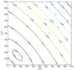
Figure 3: Initial positions of the sensor ($\diamondsuit$) and targets ($\square$). The contours depict the sensor’s detection profile presented in (18), in which the detection probability decreases with distance from the sensor.

The single-target transition density is $f({x}_{k}|{x}_{k-1})=\mathcal{N}({x}_{k};{F}{x}_{k-1},{Q})$, where

$${F}=\begin{bmatrix}1&0&T&0\\ 0&1&0&T\\ 0&0&1&0\\ 0&0&0&1\end{bmatrix},\;{Q}=27\begin{bmatrix}T^{3}&0&\frac{T^{2}}{54}&0\\ 0&T^{3}&0&\frac{T^{2}}{54}\\ \frac{T^{2}}{54}&0&\frac{T}{81}&0\\ 0&\frac{T^{2}}{54}&0&\frac{T}{81}\end{bmatrix}$$

with $T=1s$.

Measurements are noisy position returns according to the single-target likelihood

$$g({z}_{k}|{x}_{k})=\mathcal{N}({z}_{k};{H}{x}_{k},{R}_{k}),$$

where

$${R}_{k}=\sigma_{\epsilon,k}^{2}\begin{bmatrix}1&0\\ 0&1\end{bmatrix}$$

with $\sigma_{\epsilon,k}=3m$.

Clutter is modeled by a Poisson RFS with intensity $\kappa({z})=\lambda c({z})$ where $\lambda=2\!\times\!10^{\!-\!5}m^{\!-\!2}$ and $c({z})=U([0,1000m]\times[0,1000m])$ is the uniform density over the surveillance area.

At time $k-1$, the set $\mathbb{A}_{k-1}$ contains all admissible control command that drive the sensor from the current position $s_{k-1}=\left[s_{k-1}^{(x)},s_{k-1}^{(y)}\right]^{T}$ to one of the following locations

$$\mathbb{S}_{k}\!=\!\left\{\!\left[s_{k\!-\!1}^{(x)}\!+\!j_{\!}\Delta_{R}\!\cos(_{\!}\ell\Delta_{\theta\!}),s_{k\!-\!1}^{(y)}\!+\!j_{\!}\Delta_{R}\!\sin(_{\!}\ell\Delta_{\theta\!})_{\!}\right]^{\!T\!}\right\}_{\!(j,\ell)=(0,0)}^{\!(N_{R},N_{\theta})},$$

where $\Delta_{\theta}=\frac{2\pi}{N_{\theta}}{rad}$ and $\Delta_{R}=50{m}$ are the angular and radial step sizes respectively. The number of angular and radial steps are $N_{R}=2$ and $N_{\theta}=8$. The set $\mathbb{S}_{k}$, thus, has $17$ options in total which discretize the angular and radial region around the current sensor position. The sensor is always kept inside the surveillance area by setting the value of the objective function corresponding to positions outside the surveillance area to $-\infty$.

With these settings, it is expected that our control policy should, intuitively speaking, move the sensor towards the targets, and remain in their vicinity in order to obtain a high detection probability. Fig. 4 depicts a typical sensor trajectory which appears to be consistent with this intuitive expectation.

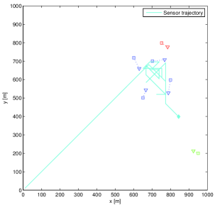
Figure 4: A typical sensor trajectory. Target start and stop positions are marked by $\square$ and $\nabla$, respectively. The red target died at $k=19$ whereas the green target was born at $k=27$. The sensor initially moved towards the targets and remained in their vicinity, then moved again to the middle of the existing targets and the new born target for optimal detection of all targets.

We proceed to illustrate the performance of the proposed strategy. First, we compare the performance of the Cauchy-Schwarz divergence based control strategy to that of an existing Rényi divergence based control strategy proposed in [26]. Since the Rényi divergence in general has no closed form solution and thus must be approximated by Sequential Monte Carlo (SMC), we also have to implement the Cauchy-Schwarz divergence using SMC approximation in order to enable a fair comparison. Second, the proposed GM implementation performance is then benchmarked against that of the SMC-based approach. When the objective function is approximated by SMC, the corresponding SMC-PHD filter [29] is used for recursive propagation of the posterior intensity function. All algorithms were implemented in MATLAB R2010b on a laptop with an Intel Core i5-3360 CPU and 8GB of RAM. The average run time for the Rényi divergence based strategy is 10.62 seconds (SMC-PHD filter implementation) while those for the Cauchy-Schwarz based strategies are 10.68 seconds (SMC-PHD filter implementation) and 3.21 seconds (GM-PHD filter implementation). It is evident that the closed form Cauchy-Schwarz divergence based strategy is the fastest.

Fig. 5 shows the Optimal SubPattern Assignment (OSPA) metric or miss distance [54] (with parameters $p=2$, $c=100m$) averaged over 200 Monte Carlo runs for each of the considered control strategies. The OSPA curves in Figure 5 suggest that the closed form GM-PHD filter based strategy outperforms its approximate SMC-PHD filter based counterparts, while the performance of the two approximate SMC-PHD filter based strategies are virtually identical.

These numerical results suggest that the Cauchy-Schwarz divergence can be at least as effective as the Rényi divergence when used as a reward function for multi-target sensor control. The results further suggest that the former has the distinct advantage of the GM implementation which leads to superior performance due to closed form solution and better filtering capability.

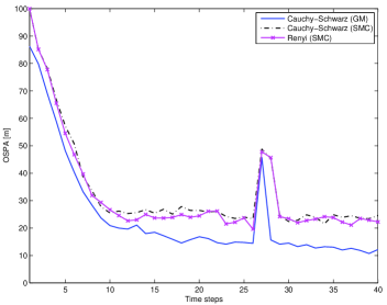
Figure 5: Comparison of the averaged OSPA distance generated by different control strategies. While SMC-PHD implementations for the Rényi divergence (dashed line) and the Cauchy-Schwarz divergence (starred line) yield similar results, they are outperformed by the GM-PHD implementation (solid line) due to closed form solution for the Cauchy-Schwarz divergence and better filtering performance.

V Conclusions

In this paper, we have extended the notion of the Cauchy-Schwarz divergence to point processes, and have shown that for an appropriate choice of reference measure, the Cauchy-Schwarz divergence between the probability densities of two Poisson point processes is half the squared distance between their intensity functions. We have extended this result to mixtures of Poisson point process and derived closed form expressions for the Cauchy-Schwarz divergence when the intensity functions are Gaussian mixtures. The Cauchy-Schwarz divergence for probability densities is not necessarily invariant to the choice of reference measure. Nonetheless the Cauchy-Schwarz divergence for the square roots of probability densities, or equivalently, the Bhattacharyya distance for probability measures, importantly is invariant to the choice of reference measure. For Poisson point processes, our result implies that the Bhattacharyya distance between the probability distributions is equal to the square of the Hellinger distance between the intensity measures, which in turn is the difference between the expected number of points per process and the Bhattacharyya coefficient of their intensity measures. We have illustrated an application of our result on a sensor control problem for multi-target tracking where the system state is modeled as a point process. Our result is an addition to the list of interesting properties of Poisson point processes and has important implications in the approximation of point processes.

Appendix A Linear Gaussian system model

In a linear Gaussian multi-target model, each constituent element $x_{k-1}$ of the multi-target state $X_{k-1}$ at time $k-1$ either continues to exist at time $k$ with probability $p_{S,k}$ or dies with probability $1-p_{S,k}$, and conditional on its existence at time $k$, transitions from $x_{k-1}$ to $x_{k}$ with probability density

$$f(x_{k}|x_{k-1})=\mathcal{N}(x_{k};F_{k-1}x_{k-1},Q_{k-1}).$$ (19)

The surviving targets at time $k$ is thus a Multi-Bernoulli point process or RFS [51, 53, 26, 52]. New targets can arise at time $k$ either by spontaneous births, or by spawning from targets at time $k-1$. The set of birth targets and spawned targets are modeled as Poisson point processes with respective Gaussian mixture intensity functions

$$\gamma_{k}(x) =\sum_{i=1}^{J_{\gamma,k}}w_{\gamma,k}^{(i)}\mathcal{N}\left(x;m_{\gamma,k}^{(i)},P_{\gamma,k}^{(i)}\right),$$

$$\beta_{k|k-1}(x|\zeta) =\sum_{i=1}^{J_{\beta,k}}w_{\beta,k}^{(i)}\mathcal{N}\left(x;F_{\beta,k-1}^{(i)}\zeta+d_{\beta,k-1}^{(i)},Q_{\beta,k-1}^{(i)}\right),$$

The multi-target state is hidden and is partially observed by a sensor driven by the control vector $a_{k-1}$ at time $k-1$. Each target evolves and generates observations independently of one another. A target with state $x_{k}$ is detected by the sensor with probability:

$$p_{D,k}(x;a_{k-1})=\sum_{j=0}^{J_{D,k}}w_{D,k}^{(j)}\mathcal{N}\left(x;m_{D,k}^{(j)}(a_{k-1}),P_{D,k}^{(j)}\right)$$

(or missed with probability $1-p_{D,k}(x_{k};a_{k-1})$) and conditional on detection generates a measurement $z_{k}$ according to the probability density

$$g_{k}(z_{k}|x_{k})=\mathcal{N}(z_{k};H_{k}x_{k},R_{k}).$$ (20)

The detections corresponding to targets is thus a Multi-Bernoulli point process [51, 53, 26, 52]. The sensor also registers a set of spurious measurements (clutter), independent of the detections, modeled as a Poisson point process with intensity $\kappa_{k}$. Thus, at each time step the measurement is a collection of detections $Z_{k}$, only some of which are generated by targets.

Appendix B Posterior intensity propagation

In general, posterior intensity function is propagated recursively in time via the Probability Hypothesis Density (PHD) filter [16]. For the linear Gaussian multi-target system described in Appendix A, the posterior intensity function is propagated via the Gaussian Mixture PHD (GM-PHD) filter [50] as follows.

Prediction: If the posterior intensity at time $k-1$ is a Gaussian mixture of the form

$$v_{k-1}(x)=\sum_{i=1}^{J_{k-1}}w_{k-1}^{(i)}\mathcal{N}(x;m_{k-1}^{(i)},P_{k-1}^{(i)})$$

then the predicted intensity at time $k$ is also a Gaussian mixture and is given by

$$v_{k|k-1}(x)=v_{S,k|k-1}(x)+v_{\beta,k|k-1}(x)+\gamma_{k}(x)$$

where

$$v_{S,k|k-1}(x) =p_{S,k}\sum_{i=1}^{J_{k-1}}w_{k-1}^{(i)}\mathcal{N}\left(x;m_{S,k|k-1}^{(i)},P_{S,k|k-1}^{(i)}\right)$$

$$v_{\beta,k|k-1}(x) =\sum_{i=1}^{J_{k-1}}\sum_{j=1}^{J_{\beta,k}}w_{k-1}^{(i)}w_{\beta,k}^{(j)}\mathcal{N}\left(x;m_{\beta,k|k-1}^{(i,j)},P_{\beta,k|k-1}^{(i,j)}\right)$$

$$m_{S,k|k-1}^{(i)} =F_{k-1}m_{k-1}^{(i)}$$

$$P_{S,k|k-1}^{(i)} =Q_{k-1}+F_{k-1}P_{k-1}^{(i)}\left[F_{k-1}\right]^{T}$$

$$m_{\beta,k|k-1}^{(i,j)} =F_{\beta,k-1}^{(j)}m_{k-1}^{(i)}+d_{\beta,k-1}^{(j)}$$

$$P_{\beta,k|-1}^{(i,j)} =Q_{\beta,k-1}^{(j)}+F_{\beta,k-1}^{(j)}P_{\beta,k-1}^{(i)}\left[F_{\beta,k-1}^{(j)}\right]^{T}.$$

Update: If predicted intensity and detection probability are Gaussian mixtures of the form

$$v_{k|k-1}(x)=\sum_{i=1}^{J_{k|k-1}}w_{k|k-1}^{(i)}\mathcal{N}\left(x;m_{k|k-1}^{(i)},P_{k|k-1}^{(i)}\right),$$

then, the posterior intensity at time $k$ is given by

$$v_{k}(x;Z_{k}(a_{k-1}))=v_{M,k}(x;a_{k-1})+\sum_{z\in Z_{k}(a_{k-1})}v_{D,k}(x;z)$$

where

$$v_{M,k}(x;a_{k-1}) =\sum_{i=1}^{J_{k|k-1}}w_{M,k}^{(i)}(a_{k-1})\mathcal{N}\left(x;m_{k|k-1}^{(i)},P_{k|k-1}^{(i)}\right)$$

$$w_{M,k}^{(i)}(a_{k-1}) =\frac{w_{\mu,k}^{(i)}(a_{k-1})T_{k}(a_{k-1})}{\displaystyle\sum_{i=1}^{J_{k|k-1}}w_{\mu,k}^{(i)}(a_{k-1})}$$

$$w_{\mu,k}^{(i)}(a_{k-1}) =\left[1-p_{D,k}\left(m_{k|k-1}^{(i)};a_{k-1}\right)\right]w_{k|k-1}^{(i)}$$

$$T_{k}(a_{k-1}) =\sum_{i=1}^{J_{k|k-1}}w_{k|k-1}^{(i)}-\sum_{i=1}^{J_{k|k-1}}\sum_{j=0}^{J_{D,k}}w_{k|k-1}^{(i,j)}(a_{k-1})$$

$$w_{k|k-1}^{(i,j)}(a_{k-1}) =w_{k|k-1}^{(i)}w_{D,k}^{(j)}q_{k|k-1}^{(i,j)}(a_{k-1}),$$

$$q_{k|k-1}^{(i,j)}(a_{k-1}) =\mathcal{N}\left(m_{D,k}^{(j)}(a_{k-1});m_{k|k-1}^{(i)},P_{k|k-1}^{(i)}+P_{D,k}^{(j)}\right),$$

and

$$v_{D,k}(x;z) =\sum_{i=1}^{J_{k|k-1}}\sum_{j=0}^{J_{D,k}}w_{k}^{(i,j)}(z)\mathcal{N}\left(x;m_{k|k}^{(i,j)}(z),P_{k|k}^{(i,j)}\right),$$

$$w_{k}^{(i,j)}(z) =\frac{w_{k|k-1}^{(i,j)}(a_{k-1})q_{k}^{(i,j)}(z)}{\kappa_{k}(z)+\displaystyle\sum_{i=1}^{J_{k|k-1}}\sum_{j=0}^{J_{D,k}}w_{k|k-1}^{(i,j)}(a_{k-1})q_{k}^{(i,j)}(z)},$$

$$q_{k}^{(i,j)}(z) =\mathcal{N}\left(z;H_{k}m_{k|k-1}^{(i,j)},R_{k}+H_{k}P_{k|k-1}^{(i,j)}H_{k}^{T}\right),$$

$$m_{k|k-1}^{(i,j)} =m_{k|k-1}^{(i)}+K_{k|k-1}^{(i,j)}\left[m_{D,k}^{(j)}(a_{k-1})-m_{k|k-1}^{(i)}\right],$$

$$P_{k|k-1}^{(i,j)} =\left[I-K_{k|k-1}^{(i,j)}\right]P_{k|k-1}^{(i)},$$

$$K_{k|k-1}^{(i,j)} =P_{k|k-1}^{(i)}\left[P_{k|k-1}^{(i)}+P_{D,k}^{(j)}\right]^{-1},$$

$$m_{k|k}^{(i,j)}(z) =m_{k|k-1}^{(i,j)}+K_{k}^{(i,j)}\left[z-H_{k}m_{k|k-1}^{(i,j)}\right],$$

$$P_{k|k}^{(i,j)} =\left[I-K_{k}^{(i,j)}H_{k}\right]P_{k|k-1}^{(i,j)},$$

$$K_{k}^{(i,j)} =P_{k|k-1}^{(i,j)}H_{k}^{T}\left(H_{k}P_{k|k-1}^{(i,j)}H_{k}^{T}+R_{k}\right)^{-1},$$

and by convention $q_{k|k-1}^{(i,0)}=1$, $m_{k|k-1}^{(i,0)}=m_{k|k-1}^{(i)}$, and $P_{k|k-1}^{(i,0)}=P_{k|k-1}^{(i)}$.

Hung Gia Hoang was born in Ha Noi, Viet Nam, in 1978. He received the B.E. degree in Electronic Engineering and Telecommunications in 2000 from Vietnam National University (VNU Hanoi) and the Ph.D. degree in Electrical Engineering in 2009 from the University of New South Wales, Australia. He is currently a Research Fellow in the Department of Electrical and Computer Engineering at Curtin University. His research interests are probabilistic methods in signal processing, control, and information theory.

Ba-Ngu Vo received his Bachelor degrees jointly in Science and Electrical Engineering with first class honors in 1994, and PhD in 1997. He had held various research positions before joining the department of Electrical and Electronic Engineering at the University of Melbourne in 2000. In 2010, he joined the School of Electrical Electronic and Computer Engineering at the University of Western Australia as Winthrop Professor and Chair of Signal Processing. Since 2012 he is Professor and Chair of Signals and Systems in the Department of Electrical and Computer Engineering at Curtin University. Prof. Vo is a recipient of the Australian Research Council’s inaugural Future Fellowship and the 2010 Australian Museum Eureka Prize for Outstanding Science in support of Defence or National Security. His research interests are Signal Processing, Systems Theory and Stochastic Geometry with emphasis on target tracking, robotics, computer vision and space situational awareness.

Ba-Tuong Vo was born in Perth, Australia, in 1982. He received the B.Sc. degree in applied mathematics and B.E. degree in electrical and electronic engineering (with first-class honors) in 2004 and the Ph.D. degree in engineering (with Distinction) in 2008, all from the University of Western Australia. He is currently an Associate Professor in the Department of Electrical and Computer Engineering at Curtin University and a recipient of an Australian Research Council Fellowship. His primary research interests are in point process theory, filtering and estimation, and multiple object filtering. Dr. Vo is a recipient of the 2010 Australian Museum DSTO Eureka Prize for ”Outstanding Science in Support of Defence or National Security”.

Ronald Mahler Ronald Mahler was born in Great Falls, MT, in 1948. He received the B.A. degree in mathematics from the University of Chicago, Chicago, IL, in 1970; the Ph.D. in mathematics from Brandeis University, Waltham, MA, in 1974; and the B.E.E. in electrical engineering from the University of Minnesota, Minneapolis, in 1980. He was an Assistant Professor of Mathematics at the University of Minnesota from 1974 to 1979. He was employed at Lockheed Martin Corp. from 1980 through 2014, where he received the 2004 and 2008 MS2 Author of the Year awards. Currently he is an independent consultant (Random Sets LLC). His research interests include information fusion, expert systems theory, multitarget tracking, and sensor management. He has authored two books and coauthored a third. Two of his papers are the first and fourth most-cited papers published in IEEE Trans. Aerospace & Electronic Systems over the last decade. He has received the 2007 Mignogna Data Fusion Award, the 2005 IEEE AESS Harry Rowe Mimno Award, and the 2007 IEEE AESS M. Barry Carlton Award.

References

- [1] H. G. Hoang, B.-N. Vo, B. T. Vo, and R. Mahler, “The Cauchy-Schwarz divergence for poisson point processes,” in Proc. IEEE Workshop on Statistical Signal Processing (SSP 2014), June 2014, pp. 240–243.
- [2] D. Daley and D. Vere-Jones, An introduction to the theory of point processes. Springer-Verlag, 1988.
- [3] D. Stoyan, D. Kendall, and J. Mecke, Stochastic Geometry and its Applications. John Wiley & Sons, 1995.
- [4] J. Kingman, Poisson Processes. Oxford University Press, 1993.
- [5] N. Van Lieshout, Markov Point Processes and Their Applications. Imperial College Press, 2000.
- [6] J. Moller and R. Waagepetersen, Statistical Inference and Simulation for Spatial Point Processes. Chapman & Hall CRC, 2004.
- [7] A. Baddeley, I. Bárány, R. Schneider, and W. Weil, Stochastic Geometry: Lectures Given at the C.I.M.E. Summer School Held in Martina Franca, Italy, September 13-18, 2004. Springer, 2007.
- [8] F. Baccelli and B. Bllaszczyszyn, “Stochastic geometry and wireless networks: Volume I Theory,” Foundation and Trends in Networking, vol. 3, no. 3-4, pp. 249–449, Mar. 2009.
- [9] D. Stoyan and A. Penttinen, “Recent applications of point process methods in forestry statistics,” Statistical Science, vol. 15, no. 1, pp. 61–78, 2000.
- [10] Y. Ogata, “Seismicity analysis through point-process modeling: A review,” Pure and applied geophysics, vol. 155, no. 2-4, pp. 471–507, 1999.
- [11] V. Marmarelis and T. Berger, “General methodology for nonlinear modeling of neural systems with Poisson point-process inputs,” Mathematical Biosciences, vol. 196, no. 1, pp. 1 – 13, 2005.
- [12] D. L. Snyder, L. J. Thomas, and M. M. Ter-Pogossian, “A mathematical model for positron-emission tomography systems having time-of-flight measurements,” IEEE Trans. Nucl. Sci., vol. 28, no. 3, pp. 3575–3583, 1981.
- [13] F. Baccelli, M. Klein, M. Lebourges, and S. A. Zuyev, “Stochastic geometry and architecture of communication networks,” Telecommunication Systems, vol. 7, no. 1-3, pp. 209–227, 1997.
- [14] M. Haenggi, “On distances in uniformly random networks,” IEEE Trans. Inf. Theory, vol. 51, no. 10, pp. 3584–3586, 2005.
- [15] M. Haenggi, J. Andrews, F. Baccelli, O. Dousse, and M. Franceschetti, “Stochastic geometry and random graphs for the analysis and design of wireless networks,” IEEE J. Sel. Areas Commun., vol. 27, no. 7, pp. 1029–1046, 2009.
- [16] R. Mahler, “Multitarget Bayes filtering via first-order multitarget moments,” IEEE Trans. Aerosp. Electron. Syst., vol. 39, no. 4, pp. 1152–1178, Oct 2003.
- [17] S. S. Singh, B.-N. Vo, A. J. Baddeley, and S. A. Zuyev, “Filters for spatial point processes.” SIAM J. Control and Optimization, vol. 48, no. 4, pp. 2275–2295, 2009.
- [18] F. Caron, P. Del Moral, A. Doucet, and M. Pace, “On the conditional distributions of spatial point processes.” Advances in Applied Probability, vol. 43, no. 2, pp. 301–307, 2011.
- [19] D. R. Cox and V. Isham, Point processes. Chapman & Hall, 1980.
- [20] T. M. Cover and J. A. Thomas, Elements of Information Theory. New York, NY, USA: Wiley-Interscience, 1991.
- [21] S. M. Ali and S. D. Silvey, “A General Class of Coefficients of Divergence of One Distribution from Another,” Journal of the Royal Statistical Society. Series B (Methodological), vol. 28, no. 1, pp. 131–142, 1966.
- [22] W. Schmaedeke, “Information based sensor management,” in Proc. SPIE Signal Processing, Sensor Fusion, and Target Recognition II, vol. 155, 1993, pp. 156–164.
- [23] R. P. S. Mahler, “Global posterior densities for sensor management,” in Proc. SPIE, vol. 3365, 1998, pp. 252–263.
- [24] S. Singh, N. Kantas, B.-N. Vo, A. Doucet, and R. Evans, “Simulation based optimal sensor scheduling with application to observer trajectory planning,” Automatica, vol. 43, no. 5, pp. 817–830, 2007.
- [25] A. O. Hero, C. M. Kreucher, and D. Blatt, “Information theoretic approaches to sensor management,” in Foundations and applications of sensor management, A. O. Hero, D. A. Castanón, D. Cochran, and K. Kastella, Eds. Springer, 2008, ch. 3, pp. 33–57.
- [26] B. Ristic, B.-N. Vo, and D. Clark, “A note on the reward function for PHD filters with sensor control,” IEEE Trans. Aerosp. Electron. Syst., vol. 47, no. 2, pp. 1521–1529, 2011.
- [27] H. G. Hoang, “Control of a mobile sensor for multi-target tracking using Multi-Target/Object Multi-Bernoulli filter,” in Proc. International Conference on Control, Automation and Information Sciences (ICCAIS 2012), Ho Chi Minh City, Vietnam, 2012, pp. 7–12.
- [28] J. D. Victor, “Spike train metrics,” Current Opinion in Neurobiology, vol. 15, no. 5, pp. 585–592, 2005.
- [29] B.-N. Vo, S. Singh, and A. Doucet, “Sequential Monte Carlo methods for multi-target filtering with random finite sets,” IEEE Trans. Aerosp. Electron. Syst., vol. 41, no. 4, pp. 1224–1245, 2005.
- [30] R. Mahler, Statistical Multisource-Multitarget Information Fusion. Artech House, 2007.
- [31] K. Kampa, E. Hasanbelliu, and J. C. Principe, “Closed-form Cauchy-Schwarz PDF divergence for mixture of Gaussians,” in Proc. International joint conference on Neural Networks (IJCNN 2011). IEEE, 2011, pp. 2578–2585.
- [32] S. Kullback and R. A. Leibler, “On information and sufficiency,” The Annals of Mathematical Statistics, vol. 22, no. 1, pp. pp. 79–86, 1951.
- [33] J. Lin, “Divergence measures based on the Shannon entropy,” IEEE Trans. Inf. Theory, vol. 37, no. 1, pp. 145–151, 1991.
- [34] F. Wang, T. Syeda-Mahmood, B. Vemuri, D. Beymer, and A. Rangarajan, “Closed-form Jensen-Rényi divergence for mixture of Gaussians and applications to group-wise shape registration,” in Medical Image Computing and Computer-Assisted Intervention MICCAI 2009. Springer, 2009, vol. 5761, pp. 648–655.
- [35] R. Jenssen, D. Erdogmus, K. E. Hild, J. C. Principe, and T. Eltoft, “Optimizing the Cauchy-Schwarz PDF distance for information theoretic, non-parametric clustering,” in Proc. 5th international conference on Energy Minimization Methods in Computer Vision and Pattern Recognition, 2005.
- [36] T. Villmann, B. Hammer, F.-M. Schleif, T. Geweniger, T. Fischer, and M. Cottrell, “Prototype based classification using information theoretic learning,” in Neural Information Processing, I. King, J. Wang, L.-W. Chan, and D. Wang, Eds. Springer Berlin Heidelberg, 2006, vol. 4233, pp. 40–49.
- [37] R. Jenssen, J. C. Principe, D. Erdogmus, and T. Eltoft, “The Cauchy-Schwarz divergence and Parzen windowing: Connections to graph theory and Mercer kernels,” Journal of the Franklin Institute, vol. 343, no. 6, pp. 614 – 629, 2006.
- [38] E. Hasanbelliu, L. Sanchez-Giraldo, and J. Principe, “A robust point matching algorithm for non-rigid registration using the Cauchy-Schwarz divergence,” in Proc. IEEE International Workshop on Machine Learning for Signal Processing (MLSP 2011), 2011, pp. 1–6.
- [39] K. DeMars, I. Hussein, M. Jah, and R. Erwin, “The Cauchy-Schwarz divergence for assessing situational information gain,” in Proc. International Conference on Information Fusion (FUSION2012), 2012, pp. 1126–1133.
- [40] C. E. Rasmussen and C. K. I. Williams, Gaussian Processes for Machine Learning. The MIT Press, 2005.
- [41] F. Le Gall, “Powers of tensors and fast matrix multiplication,” in Proc. 39th International Symposium on Symbolic and Algebraic Computation, ser. ISSAC ’14, 2014, pp. 296–303.
- [42] J.-H. Lo, “Finite-dimensional sensor orbits and optimal nonlinear filtering,” IEEE Trans. Inf. Theory, vol. 18, no. 5, pp. 583–588, 1972.
- [43] C. Ji, D. Merl, T. B. Kepler, and M. West, “Spatial mixture modelling for unobserved point processes: Examples in immunofluorescence histology,” Bayesian Analysis, vol. 4, pp. 297–316, 2009.
- [44] A. Kostas and S. Behseta, “Bayesian nonparametric modeling for comparison of single-neuron firing intensities,” Biometrics, vol. 66, pp. 277–286, 2010.
- [45] M. Taddy, “Autoregressive mixture models for dynamic spatial Poisson processes: Application to tracking intensity of violent crime,” Journal of the American Statistical Association, vol. 105, pp. 1403–1417, 2010.
- [46] D. Phung and B.-N. Vo, “A random finite set model for data clustering,” in Proc. International Conference on Information Fusion (FUSION 2014), July 2014, pp. 1–8.
- [47] A. Bhattacharyya, “On a measure of divergence between two statistical populations defined by their probability distribution,” Bulletin of the Calcutta Mathematical Society, vol. 35, pp. 99–110, 1943.
- [48] T. Kailath, “The divergence and Bhattacharyya distance measures in signal selection,” IEEE Trans. Inf. Theory, vol. 15, no. 1, pp. 52–60, 1967.
- [49] I. R. Goodman, R. Mahler, and H. T. Nguyen, Mathematics of Data Fusion. Kluwer Academic Publishers, 1997.
- [50] B.-N. Vo and W.-K. Ma, “The Gaussian mixture probability hypothesis density filter,” IEEE Trans. Signal Process., vol. 54, no. 11, pp. 4091–4104, 2006.
- [51] R. Mahler, “Multitarget sensor management of dispersed mobile sensors,” in Theory and algorithms for cooperative systems, D. Grundel, R. Murphey, and P. Pardalos, Eds. World Scientific Books, 2004, ch. 12, pp. 239–310.
- [52] H. G. Hoang and B. T. Vo, “Sensor management for multi-target tracking via multi-Bernoulli filtering,” Automatica, vol. 50, no. 4, pp. 1135–1142, 2014.
- [53] B. Ristic and B.-N. Vo, “Sensor control for multi-object state-space estimation using random finite sets,” Automatica, vol. 46, no. 11, pp. 1812–1818, 2010.
- [54] D. Schumacher, B.-T. Vo, and B.-N. Vo, “A consistent metric for performance evaluation of multi-object filters,” IEEE Trans. Signal Process., vol. 56, no. 8, pp. 3447–3457, 2008.
- [55] M. Ulmke, O. Erdinc, and P. Willett, “GMTI tracking via the Gaussian Mixture Cardinalized Probability Hypothesis Density filter,” IEEE Trans. Aerosp. Electron. Syst., vol. 46, no. 4, pp. 1821–1833, 2010.