Laser Doppler Imaging of Microflow
Abstract
We report a pilot study with a wide-field laser Doppler detection scheme used to perform laser Doppler anemometry and imaging of particle seeded microflow. The optical field carrying the local scatterers (particles) dynamic state, as a consequence of momentum transfer at each scattering event, is analyzed in the temporal frequencies domain. The setup is based on heterodyne digital holography, which is used to map the scattered field in the object plane at a tunable frequency with a multipixel detector. We show that wide-field heterodyne laser Doppler imaging can be used for quantitative microflow diagnosis; in the presented study, maps of the first-order moment of the Doppler frequency shift are used as a quantitative and directional estimator of the Doppler signature of particles velocity.
1Laboratoire Kastler-Brossel, Ecole Normale Supérieure, UMR 8552 (ENS, CNRS, UMPC), 24 rue Lhomond 75231 Paris cedex 05. France
2Laboratoire Microfluidique, MEMS, Nanostructures, ESPCI, CNRS UPR A0005, Université Pierre et Marie Curie, 10 rue Vauquelin 75005 Paris. France.
Keywords: Laser Doppler anemometry, microflow, Doppler imaging
Citation:
M. Atlan, M. Gross and J. Leng. ”Laser Doppler imaging of microflow” Journal of the European Optical Society - Rapid publications, 1, 06025 (2006)
[DOI: 10.2971/jeos.2006.06025]
1 Introduction: Velocimetry and microfluidics
Microfluidics has emerged as an important tool for engineering, fundamental science, biology, etc. [1]. The ability to control flow patterns at a typical scale of a micrometer through advanced microfabrication techniques [2] offers a neat and powerful guide for the development of analytical microfluidics chips. Of primary importance is the charaterization of flow patterns in microsystems [3] and much of the technological effort has focused on direct determination of flow profiles of liquids inside micro-capillaries. The size reduction indeed precludes the use of external probes and therefore dismisses most of traditional macroscopic techniques for velocimetry (eg. hot-wire anemometry [4]). Particle-based flow visualization techniques (particle image velocimetry (PIV) [5], that often use fluorescent microspheres of a size of order of 100 nm in dilute suspensions at volume fraction of order of 10.5) are popular as little intrusive tools that offer high spatial resolution in the characterization of local flow properties (especially -PIV, for biological or complex fluids [6] [8] and biphasic flows [9]). Holographic configurations have been used for particle field diagnosis [10] and velocimetry [11, 12]. Digital holographic PIV (HPIV) constitutes an active field of research, where off-axis HPIV appears to be a better configuration than inline HPIV in terms of signal-to-noise ratio (SNR) [13, 14]. Other visualisation techniques, based on fluorescence bleaching [15], correlation spectroscopy [16], caged fluorescence [17], molecular tagging velocimetry [18], total internal reflection fluorescence [19, 20], etc., are also used to investigate local flow properties.
In conventional laser Doppler velocimetry (LDV), the scattered laser light coming from a focus point onto a sample is detected by a single detector and analyzed by a spectrum analyzer. The power spectrum of coherent monochromatic light scattered by moving particles is broadened as a result of momentum transfer. The resulting broadening of light is linked to the velocity distribution of scatterers [21, 22]. Doppler maps can be realized by scanning the focus point on the sample surface, which constitutes the principle of scanning Laser Doppler Imaging (LDI) [23] [25], for which spatial resolution is typically low. Although LDV is a standard technique for macroflow studies, several difficulties limit its use in microflow: The focusing point of the laser beam has to be very accurately controlled, its micron-scale extension limits the accuracy of the velocity measurements, and the temporal resolution diminishes with the spatial scale of the sample [3, 26].
We designed a parallel imager aimed at LDI [27], alleviating the issue of spatial scanning. Our technique involves a frequency selective heterodyne detection of the light on a multi pixel CCD detector which records digital holograms in an off axis configuration. The image is reconstructed numerically by using standard numerical holography algorithms. By sweeping the optical frequency of heterodyne detection local oscillator (reference arm), we record the spatial distribution of tunable frequency components of the object field sequentially.We demonstrate here that the technique can be employed as a tool for in-plane flow analysis in microfluidic networks and is especially well-suited for building up Doppler maps (absolute values along with gradient measurements) on intermediate scale ( 1 cm) microfluidics webs.
Our technique can be interpreted as a Doppler global (or planar) velocimetry (DGV) measurement, but on a very different temporal frequency scale than molecular absorption-based DGV [28, 29]. Molecular absorption DGV relies on the absorption characteristics of iodine vapor to convert a Doppler shift to a recordable intensity. Because of the characteristics of the absorption curve of the iodine and the finite stability of laser cavities, the frequency resolution is 1 MHz (velocity resolution of 1 m/s) [30], and is therefore not suitable for microflow analysis. In our case, the measurement relies on a heterodyne detection extremely selective in frequency. the detection bandwidth is the reciprocal of the measurement time, hence a frequency resolution of a few Hz, compatible with microflow analysis. Our method also differentiates itself from scanning LDI and HPIV methods. Whereas scanning LDI performs sequential measurements in space and parallel measurements in the temporal frequency domain, our instrument does parallel measurements in space and sequential measurements in frequency. And unlike HPIV and its refinements (e.g. [31]), our technique does not rely on the localization of the seeding particles onto an image. Like in DGV, Doppler maps are the result of a direct selective measurement of frequency-shifted components of the scattered light. The advantages of our heterodyne holography method for wide field laser Doppler measurements are the sensitivity (heterodyne gain), the selectivity in the temporal frequency domain (coherent detection) and the large optical étendue (product of the detector area by the detection solid angle) of multi pixel coherent detection [32, 33].
2 Optical Setup
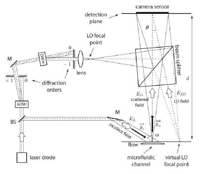
The experimental setup [27, 34] is based on an optical interferometer sketched in Figure 1.A CW, 80mW, = 658 nm diode (Mitsubishi ML120G21) provides the main laser beam, split by a prism into a reference (local oscillator, LO) and an object arm. The dimensionless scalar amplitudes of the fields are noted (incident field), (scattered, object field) and (LO field). The object is illuminated by the laser beam with an incidence angle a. Scattered light is mixed with the reference beam and detected by a PCO PixelFly 1.3 Mpix CCD camera (1280 1024 square pixels, pixel size: 6.7 m, framerate = 4 Hz, exposure time = 125 ms), set at a distance cm from the object. Two Bragg cells (acousto-optic modulators, AOM, Crystal Technology) are used to shift the LO by a tunable frequency (the difference of their driving frequencies). A 10 mm focal length lens is placed in the reference arm in order to create an off-axis ( tilt angle) virtual point source in the object plane (see Figure 1). This configuration constitutes a lensless Fourier holography setup [35].
To perform a heterodyne detection of a frequency component of the object field, the LO field frequency is detuned by with respect to the main laser beam frequency . The shift allows the LO field to match the part of the object field shifted by . The additional shift at the n-submultiple of the camera sampling frequency provokes a modulation of the interference pattern sampled by the detector at .
The measured power spectrum S associated to the field EO is [27]:
| (1) |
Where A is a positive constant. The Dw spectral point is readout from a sequence of n images recorded by the camera [27]. EO is recorded in the detector plane by the frequencyshifting technique [32] which is the dynamic equivalent of the phase-shifting digital holography technique [36]. The lensless Fourier holographic setup [35] used here is less demanding in numerical calculations than the general Fresnel holography configuration. The numerical reconstruction algorithm of the image is limited to one discrete Fourier transform [37, 38]. Artefacts due to the finite size of the sensor and the spatial discrete Fourier transform are negligible [39] (narrower than one pixel in the reconstructed image).
We define the signal represented on spectra profiles and maps:
| (2) |
where is the quantity assessed in a region of the reconstructed hologram where the object light contribution is null. It was reported to be shot-noise dominated [33].
To map the projection of velocities with the in-plane component of the incident field wavevector (according to Eq. 4), we compute the first moment of the frequency shift :
| (3) |
where is the zeroth-order moment. These sums are calculated over the full range of measured shifts.
3 Microfluidic devices with velocity gradients
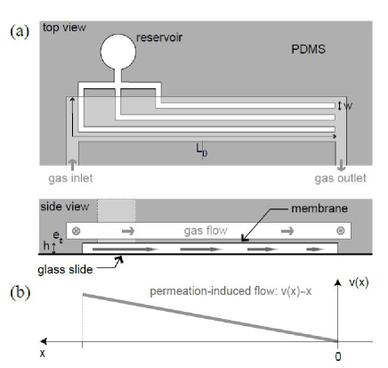
In this study, we designed a fluidic network made using standard microfabrication techniques [2]: a circuit is patterned onto a silicon substrate using micro-photolithography (spincoating of a photoresist exposed to UV s through a mask and developped to obtain hard patterns resolved at ), molded into a transparent elastomer poly-dimethylsiloxane (PDMS) and stuck on a glass substrate. We thus obtain closed circuits for liquid transport of typical dimensions 10 50 5000 . The actual devices we use are special (Figure 2) as they generate a flow via evaporation in a dead end microchannel [40], with a flow field which varies in space. Details for fabrication of these 2-layer systems (one layer for liquid transport, one layer for gas transport for evaporation) are given elsewhere [41] and the main feature we shall retain is the linear dependence of mean velocity in a channel as a function of position (while by design [40], these devices are used to concentrate a solute near the dead end of the channels, an effect we shall also evidence here). Such a heterogeneous flow field is a specificity of permeation-induced flows [42], and we will exploit it for testing the construction of velocity maps.
The microsystems are filled with a solution of pure water seeded with 1.0 m diameter latex spheres (with carboxylate stabilizing surface groups, by Molecular Probes). Evaporation induces a permanent flow that drives the liquid from the reservoir towards the dead end of the channel, with a velocity slowing down linearly from m/s down to 0 (see Figure 2). This result holds for the mean velocity; two effects alter this simple view: the flow field actually shows a parabolic profile (Poiseuille flow) and the particles undergo Brownian dynamics.
4 Wide field Laser Doppler mapping of microfluidic webs
A volumic concentration suspension of latex beads is perfused through the microfluidic web. This concentration of latex corresponds to particles per cubic micron, which was the lowest seeding for which those particles would lead to an acceptable SNR, in our configuration. A Mie algorithm 111from C. Maetzler, iapmw.unibe.ch was used to assess its optical parameters : the resultant mean free path is mm, and the anisotropy coefficient is . This suspension of latex beads was perfused in the microfluidic device, composed of 6 channels of cross section, which optical thickness (defined as the thickness of the channel in mean free path units) is much smaller than unity. The incidence angle a of the laser beam (see Figure 1) is . In this experiment, Doppler shift maps were measured in the -64 Hz +64 Hz range (spacing interval : 2 Hz). was calculated with a image demodulation and averaged over a image sequence. Here : , . The total measurement time of the spectral cube took 8 minutes and 30 seconds (= 16 images 65 frequency shifts 1/4 second exposure time). Nevertheless, in these conditions, the measurement of one complete spectral map at an arbitrary frequency shift took only 16 1/4 = 4 seconds.
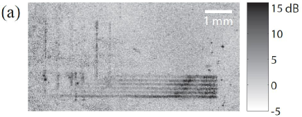
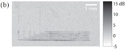
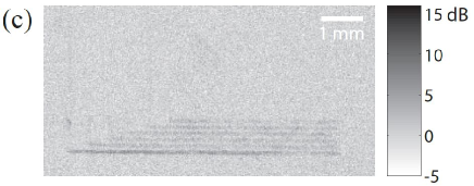
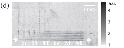
Three maps, measured at = 0, -22 and -44 Hz are represented on Figures 3a to c. The whole microfluidic web appears to respond at each arbitrary frequency. Such maps are difficult to interpret, since they represent a signal which combines both scatterers density and Doppler signature. Additionally, these results reveal an averaged response over the height of the channel. The zeroth-order moment map of the frequency shift, represented on Figure 3d, displays a signal allegedly proportional to the moving particles concentration [43] (under the approximation of a small scatterers densities), which shows the expected increase in density at the end of the channels, in region (vi).
The Doppler shift for one scattering event by a particle in translation with velocity v is [44] :
| (4) |
where is the momentum transfer, is the incident wave vector, ks the scattered wave vector and v the scatterer instant velocity. In the chosen optical configuration (Figure 1), = 0. Hence the Doppler shift in a region where the average speed of the particles is :
| (5) |
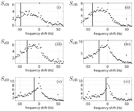
At the entrance of the longest canal (canal (1) in Figure 5a) the particles translation speed is . According to the linear behaviour [40] of , the expected flow-induced Doppler shift for each region of interest (ROI) defined in Figure 3b is represented by a vertical marker in Figures 4i to vi, at values ranging linearly from 49.2 Hz (i) to 4.4 Hz (vi), superimposed on each corresponding spectrum.
In diluted samples (in very good approximation the ones which optical thickness is much lower than 1), the root mean square (RMS) Doppler shift of light scattered by a particle undergoing brownian motion is whereis the spatial diffusion coefficient of the brownian particle; in the particular case of a spherical particle of radius , its expression is : , where is the Boltzmann constant and the absolute temperature. For our latex beads in suspension in water (of viscosity Pa.s), at room temperature ( J), we have . The average value of , for a scattering angle ( is [45]:
| (6) |
which gives, in the chosen optical configuration (Figure 1):
| (7) |
where is the incidence angle of light in water of refractive index , and is the optical wavelength in water. The numerical value of is Hz.
This value of the RMS brownian motion-induced Doppler shift is compatible with the width observed, in Figure 4vi, where the fluid velocity is nearly zero. In other regions : (i) to (v), the observed spectrum corresponds to the convolution of the brownian spectrum with the spectrum associated to the distribution of velocities in the flow (Poiseuille flow). The narrow peak, observed on the spectra near zero frequency, is a parasitic signal not related to the flow (light scattered by the PDMS substrate…).
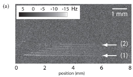
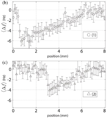
Figure 5 represents the first moment of the Doppler shift with respect to the measured Doppler linewidths on each pixel, mapped and plotted versus the longitudinal position along two microfluidic channels. Figure 5b and 5c show a linear decrease of with the position along channels (1) and (2), highlighted in Figure 5a. This corresponds to the expected linear decrease of the average velocity along the channels.
5 Conclusion
We have presented a wide field laser Doppler measurement in a microfluidic device, and demonstrated that the velocity resolution is compatible with microflow diagnosis. In the reported pilot study, the setup, based on off-axis heterodyne holography, performs a parallel measurement of the power spectrum of the light scattered by a microfluidic device on a CCD camera. The scheme is different from conventional laser Doppler time-domain measurements : each frequency point of the spectrum is acquired at a time, by tuning the LO frequency at the desired shift. Since the spectrum is processed optically, by an interferometric scheme between scattered light and a detuned local oscillator, the span of the measurable spectrum is not limited by the detector bandwidth. Furthermore, the optical configuration allows to measure algebraic Doppler shifts since the hologram records the optical field in quadrature, rather than its intensity.
In this paper, the stress was put on the potential of the wide field laser Doppler instrument in terms of frequency (and hence velocity) diagnosis : high frequency resolution, high SNR, high dynamic range of restituable frequencies on the same image, and directional discrimination. The scope of the presented study was to provide measurements in large scale microfluidic devices into which large velocity gradients can be created at the same time.
The spatial resolution of the digital holography-based apparatus is about the extent of 1 pixel on the reconstructed image [37]. Much better resolution (at the expense of the field of view) can be obtained by using an holographic microscopy configuration, which enables theoretically sub-micronic lateral resolution [46] (up to the diffraction limit). Nevertheless, time-averaged measurements of rarefied seeds at low spatial scales, might become noisy and reduce the spatial resolution of velocity maps.
The frequency resolution is given by the heterodyne bandwidth of the detection (the inverse of the total acquisition time of the image sequence). Although measured spectra are stained by the Doppler linewidth contribution of Brownian movement, the setup has an intrinsic ability to map small velocities (up to 10 micron per second, but the actual limit should be even lower, thanks to the heterodyne selectivity). Since these (and lower) flow velocities are commonly encountered in microfluidic webs, our frequency-domain wide-field laser Doppler imager appears to be a valuable candidate for microflow visualization and analysis.
The authors acknowledge support from the French ANR.
References
- [1]
[1] H. A. Stone, A. D. Stroock, and A. Ajdari, Engineering flows in small devices: Microfluidics toward a lab-on-a-chip Annual Review Of Fluid Mechanics 36, 381 411 (2004).
[2] G. M. Whitesides, E. Ostuni, S. Takayama, X. Y. Jiang, and D. E. Ingber, Soft lithography in biology and biochemistry Annual Review Of Biomedical Engineering 3, 335 373 (2001).
[3] D. Sinton, Microscale flow visualization Microfluidics and Nanofluidics 1, 2 21 (2004).
[4] G. Comte-Bellot, Hot-wire anemometry Annual Review Of Fluid Mechanics 8, 209 231 (1976).
[5] S. Kurada, G. W. Rankin, and K. Sridhar, Particle-imaging techniques for quantitative flow visualization - a review Optics And Laser Technology 25(4), 219 233 (1993).
[6] H. Muller-mohnssen, D. Weiss, and A. Tippe, Concentration dependent changes of apparent slip in polymer-solution flow Journal Of Rheology 34(2), 223 244 (1990).
[7] J. G. Santiago, S. T. Wereley, C. D. Meinhart, D. J. Beebe, and R. J. Adrian, A particle image velocimetry system for microfluidics Experiments In Fluids 25(4), 316 319 (1998).
[8] A. F. Mendez-Sanchez, J. Perez-Gonzalez, L. de Vargas, J. R. Castrejon-Pita, A. A. Castrejon-Pita, and G. Huelsz, Particle image velocimetry of the unstable capillary flow of a micellar solution Journal Of Rheology 47(6), 1455 1466 (2003).
[9] F. Innings and C. Tragardh, Visualization of the drop deformation and break-up process in a high pressure homogenizer Chemical Engineering & Technology 28(8), 882 891 (2005).
[10] BJ Thompson, JH Ward, and WR Zinky, Application of holographic techniques for particle sizing analysis Applied Optics 6(3), 519 (1967).
[11] JD Trolinger, RA Belz, and WM Farmer, Holographic techniques for the study of dynamic particle fields Applied Optics 8(5), 957 (1969).
[12] LM Weinstein, GB Beeler, and AM Lindemann, High-speed holocinematographic velocimeter for studying turbulent flow control physics American Institute of Aeronautics and Astronautics AIAA- 526 (1985).
[13] H. Meng, W.L. Anderson, F. Hussain, and D. D. Liu, Intrinsic speckle noise in in-line particle holography Optical Society of America Journal A 10, 2046 2058 (1993).
[14] H Meng and F Hussain, In-line recording and off-axis viewing technique for holographic particle velocimetry Applied Optics 34, 1827 (1995).
[15] B. P. Mosier, J. I. Molho, and Santiago J. G, Photobleachedfluorescence imaging of microflows Experiments In Fluids 33(4), 545 554 (2002).
[16] C. Ybert, F. Nadal, R. Salome, F. Argoul, and L. Bourdieu, Electrically induced microflows probed by fluorescence correlation spectroscopy European Physical Journal E 16(3), 259 266 (2005).
[17] W. R. Lempert, K. Magee, P. Ronney, K. R. Gee, and R. P. Haugland, Flow tagging velocimetry in incompressible-flow using photoactivated nonintrusive tracking of molecular-motion (phantomm) Experiments In Fluids 18(4), 249 (1995).
[18] B. Stier and M. M. Koochesfahani, Molecular tagging velocimetry (mtv) measurements in gas phase flows Experiments in Fluids V26(4), 297 304 (1999).
[19] C. Zettner and M. Yoda, Particle velocity field measurements in a near-wall flow using evanescent wave illumination Experiments in Fluids V34(1), 115 121 (2003).
[20] K. D. Kihm, A. Banerjee, C. K. Choi, and T. Takagi, Near-wall hindered brownian diffusion of nanoparticles examined by threedimensional ratiometric total internal reflection fluorescence microscopy (3-d r-tirfm) Experiments in Fluids V37(6), 811 824 (2004).
[21] R. Bonner and R. Nossal, Model for laser doppler measurements of blood flow in tissue Applied Optics 20, 2097 2107 (1981).
[22] J. D. Briers, Laser doppler and time-varying speckle: a reconciliation Optical Society of America Journal A 13, 345 (1996).
[23] H Nakase, OS Kempski, A Heimann, T Takeshima, and J. Tintera, Microcirculation after cerebral venous occlusions as assessed by laser doppler scanning J. Neurosurg. 87(2), 307 314 (1997).
[24] Beau M. Ances, Joel H. Greenberg, and John A. Detre, Laser doppler imaging of activation-flow coupling in the rat somatosensory cortex NeuroImage, 10(6), 716 723 (1999). [25] Ralf Steinmeier, Imre Bondar, Christian Bauhuf, and Rudolf Fahlbusch, Laser doppler flowmetry mapping of cerebrocortical microflow: Characteristics and limitations NeuroImage 15(1), 107 119 (2002).
[26] C.D. Meinhart, S.T. Wereley, and J.G. Santiago, Micron-Resolution Velocimetry Techniques, in Developments in Laser Techniques and Applications to Fluid Mechanics, (Springer, 1998).
[27] M. Atlan and M. Gross, Laser doppler imaging, revisited Review of Scientific Instruments 77(11), 2006.
[28] H. Komine and S. J. Brosnan, Instantaneous, three-component, doppler global velocimetry pages 273 277 (1991).
[29] J. Meyers and H. Komine, Doppler global velocimetry: A new way to look at velocity Laser Anemometry 1, 289 (1991).
[30] James F Meyers, Joseph W Lee, and Richard J Schwartz, Characterization of measurement error sources in doppler global velocimetry Measurement Science and Technology 12(4), 357 368 (2001).
[31] C.-T Yang and H.-S Chuang, Measurement of a microchamber flow by using a hybrid multiplexing holographic velocimetry Experiments in Fluids V39(2), 385 396 (2005).
[32] F. LeClerc, L. Collot, and M. Gross, Numerical heterodyne holography with two-dimensional photodetector arrays Optics Letters 25(10), 716 718 (2000).
[33] M. Gross, P. Goy, and M. Al-Koussa, Shot-noise detection of ultrasound-tagged photons in ultrasound-modulated optical imaging Optics Letters 28, 2482 2484 (2003).
[34] M. Atlan, M. Gross, T. Vitalis, A. Rancillac, B. C. Forget, and A. K. Dunn, Frequency-domain, wide-field laser doppler in vivo imaging Optics Letters 31(18) (2006).
[35] George W. Stroke, Lensless fourier-transform method for optical holography Applied Physics Letters 6(10), 201 203 (1965).
[36] U. Schnars and W. Juptner, Direct recording of holograms by a ccd target and numerical reconstruction Applied Optics 33, 179 181 (1994).
[37] Christoph Wagner, Sonke Seebacher, Wolfgang Osten, and Werner Juptner, Digital recording and numerical reconstruction of lensless fourier holograms in optical metrology Applied Optics 38, 4812 4820 (1999).
[38] U. Schnars and W. P. O. Juptner, Digital recording and numerical reconstruction of holograms Meas. Sci. Technol. 13, R85 R101 (2002).
[39] Thomas M. Kreis, Frequency analysis of digital holography Optical Engineering 41(4), 771 778 (2002).
[40] J. Leng, B. Lonetti, P. Tabeling, M. Joanicot, and A. Ajdari, Microevaporators for the kinetic inspection of phase diagrams Physical Review Letters 96(8), 084503 (2006).
[41] J. Goulpeau, D. Trouchet, A. Ajdari, and P. Tabeling, Experimental study and modeling of polydimethylsiloxane peristaltic micropumps Journal of Applied Physics 98(4) (2005).
[42] E. Verneuil, A. Buguin, and P. Silberzan, Permeation-induced flows: Consequences for silicone-based microfluidics Europhysics Letters 68(3), 412 418 (2004).
[43] A. Serov, W. Steenbergen, and F. de Mul, Laser doppler perfusion imaging with complementary metal oxide semiconductor image sensor Optics Letters 27, 300 (2002).
[44] Y. Yeh and H. Z. Cummins, Localized fluid flow measurements with an he-ne laser spectrometer Appl. Phys. Lett. 4, 176 179 (1964).
[45] B. J. Berne and R. Pecora, Dynamic Light Scattering, (Dover, 2000).
[46] Ichirou Yamaguchi, Jun ichi Kato, Sohgo Ohta, and Jun Mizuno, Image formation in phase-shifting digital holography and applications to microscopy Applied Optics 40(34), 6177 6186 (2001). 06025-