Sensor management for multi-target tracking via Multi-Bernoulli filtering

Abstract

In multi-object stochastic systems, the issue of sensor management is a theoretically and computationally challenging problem. In this paper, we present a novel random finite set (RFS) approach to the multi-target sensor management problem within the partially observed Markov decision process (POMDP) framework. The multi-target state is modelled as a multi-Bernoulli RFS, and the multi-Bernoulli filter is used in conjunction with two different control objectives: maximizing the expected Rényi divergence between the predicted and updated densities, and minimizing the expected posterior cardinality variance. Numerical studies are presented in two scenarios where a mobile sensor tracks five moving targets with different levels of observability.

, ,

1 Introduction

Multi-target sensor control/management is essentially an optimal non-linear control problem. The goal of multi-target sensor management is to “direct the right sensor on the right platform to the right target at the right time” [7]. However, the multi-target sensor control problem differs from the classical control problem in that it deals with highly complex multi-object stochastic systems. In multi-object stochastic systems, not only do the number of objects vary randomly in time, but the measurements are subject to missed detections and false alarms. This means that the multi-target state and multi-target observation are inherently finite-set-valued. Consequently, standard optimal control techniques are not directly applicable [8]. Nonetheless, the multi-target sensor scheduling problem can still be cast in the framework of partially observed Markov decision processes (POMDPs), where the states and observations are instead finite-set-valued, and control vectors are drawn from a set of admissible sensor actions based on the current information states, which are then judged against the values of an objective function associated with each action [1].

A unified approach to characterizing systems with finite-set-valued states is the multi-object systems framework, where uncertainty is described by multi-object probability density functions, and formalized via point process theory [2, 16], or equivalently by random finite set (RFS) theory through Mahler’s finite set statistics (FISST) [10]. The key advantage of the RFS based approach is that of a principled framework for modelling, estimation and control of multi-object systems. In this paper, we formulate the sensor control problem as a POMDP with an information-theoretic objective function as well as finite-set-valued states and measurements. In essence, our approach can be summarized by three basic steps:

1. Modelling the sensor and targets as a multi-object stochastic system, i.e. the multi-target states and multi-target observations as RFSs

2. Propagating the multi-object posterior density recursively in time, or alternatively a tractable approximation to the posterior;

3. At each time, determining the control action based on optimization of the reward function over a set of admissible actions.

In the context of single-target tracking, the work in [3] is the first to propose a practical particle implementation based on the Kullback-Leibler divergence, and the approach in [15] further considers the issue of observer trajectory planning. In the more difficult multi-target context, there are a handful of works falling within the RFS framework. Using the Rényi divergence as the reward function, in [12] the particle multi-object Bayes filter [18] is used to propagate the multi-object posterior, while in [13] the particle probability hypothesis density (PHD) filter [18] is used to propagate the first moment of the multi-object posterior.

This paper adopts an information theoretic approach for multi-target sensor control, similar to the approach in [12, 13], except that the Cardinality Balanced Multi-Target Multi-Bernoulli (CB-MeMBer) filter [20] is used to propagate a parametrized approximation to the multi-object posterior. The proposed approach is attractive in that it is applicable to general non-linear non-Gaussian models, and when coupled with a particle implementation further reduces the computational load significantly. Propagating an approximate multi-Bernoulli posterior as proposed is drastically cheaper than propagating the full multi-object posterior as in [12], and thus the computation of any associated cost function using a multi-Bernoulli approximation is generally cheaper than using the full posterior. While the proposed use of the CB-MeMBer filter incurs the same complexity as the use of the PHD filter for the same purpose in [13], performing state estimation with the former is more efficient and reliable than the latter because the need for clustering is eliminated. The work in [12, 13] also demonstrates that the Rényi divergence can be used as a reward function for multi-target sensor control. In the same regard, the use of the CB-MeMBer filter equally allows the Rényi divergence to be used as a reward function, and further allows a new type of the reward function to be developed. Since the variance of the estimated cardinality of a multi-Bernoulli posterior can be evaluated in closed form [10], minimizing the cardinality variance can be used as the control objective, thereby enabling direct control of the cardinality estimation error.

The main contribution of this paper is a computationally efficient sensor control algorithm for multiple targets, using the CB-MeMBer filter, as well as the numerical assessment of two types of control objectives. Our preliminary result, in particular the idea of using the CB-MeMBer filter, has been reported in the conference paper [5]. The current paper provides full details of the algorithm, an alternative cheaper control objective, and more complete numerical studies.

The organization of the paper is as follows. In Section 2 we review RFS modelling of multi-object systems and the approximation of the multi-object posterior density using the CB-MeMBer filter. The two reward functions are discussed in Section 3 while sequential Monte Carlo (SMC) implementation is described in Section 4. Section 5 presents simulation results and finally, Section 6 concludes the paper.

2 Cardinality Balanced MeMBer filter

In this section, we summarize the CB-MeMBer filter, the main tool that will be used throughout the paper. The filter was originally introduced in [20] to account for the cardinality bias of the MeMBer filter in [10].

2.1 General system model

In contrast with single-object systems where the states and observations are modelled by random vectors, the states and observations of a multi-object system are random finite sets of vectors in the single-object state space $\mathcal{X}\subseteq\mathbb{R}^{n}$ and single-object observation space $\mathcal{Z}\subseteq\mathbb{R}^{m}$, respectively:

$$\mathbf{X}_{k} =\{\mathbf{x}_{1}^{k},\ldots,\mathbf{x}_{n}^{k}\}\in\mathcal{F}(\mathcal{X});$$ (1)

$$\mathbf{Z}_{k} =\{\mathbf{z}_{1}^{k},\ldots,\mathbf{z}_{m}^{k}\}\in\mathcal{F}(\mathcal{Z}).$$ (2)

Here $\mathcal{F}(\mathcal{X})$ and $\mathcal{F}(\mathcal{Z})$ denote the spaces of all finite subsets of $\mathcal{X}$ and $\mathcal{Z}$. The system is described by the following probabilistic state space model:

$$\mathbf{X}_{k} \sim\pi_{k|k-1}(\mathbf{X}_{k}|\mathbf{X}_{k-1})$$ (3)

$$\mathbf{Z}_{k} \sim g_{k}(\mathbf{Z}_{k}|\mathbf{X}_{k})$$ (4)

where $\mathbf{X}_{k}$ and $\mathbf{Z}_{k}$ respectively are the state and observation of the system at time $k$. Equation (3) describes the system dynamics encapsulating all aspects of object birth, death and transition while equation (4) encapsulates all aspects of sensor detection and false alarms.

Given the system model (3)-(4), the objective is to determine at each time step $k$ the multi-object posterior probability density $f_{k}(\mathbf{X}_{k}|\mathbf{Z}_{1:k})$. In the Bayesian filtering framework, $f_{k}(\mathbf{X}_{k}|\mathbf{Z}_{1:k})$ is obtained through two steps: time prediction and measurement update [10]. The predicted density at time $k$ , denoted as $f_{k|k-1}(\mathbf{X}_{k}|\mathbf{Z}_{1:k-1})$, is computed by the multi-object Chapman-Kolmogorov equation:

$$f_{k|k-1}(\mathbf{X}_{k}|\mathbf{Z}_{1:k-1})=\\ \int\pi_{k|k-1}(\mathbf{X}_{k}|\mathbf{X}_{k-1})f_{k-1}(\mathbf{X}_{k-1}|\mathbf{Z}_{1:k-1})\delta\mathbf{X}_{k-1}$$ (5)

where $f_{k-1}(\mathbf{X}_{k-1}|\mathbf{Z}_{1:k-1})$ is the posterior density from the previous time step $k-1$. When new observations arrive at the sensor(s), the new posterior density is computed via the multi-object Bayes rule:

$$f_{k}(\mathbf{X}_{k}|\mathbf{Z}_{1:k})=\frac{g_{k}(\mathbf{Z}_{k}|\mathbf{X}_{k})f_{k|k-1}(\mathbf{X}_{k}|\mathbf{Z}_{1:k-1})}{\int g_{k}(\mathbf{Z}_{k}|\mathbf{X}_{k})f_{k|k-1}(\mathbf{X}_{k}|\mathbf{Z}_{1:k-1})\delta\mathbf{X}_{k}}$$ (6)

Notice that the integrals in (5) and (6) are not ordinary integrals, but are set integrals, and that the recursion (5) and (6) has no analytic solution in general. A sequential Monte Carlo (SMC) implementation of the Bayes multi-object filter is given in [18]. However, this technique is computationally prohibitive which at best is able to accommodate a small number of targets. The multi-target sensor scheduling algorithm proposed in [12] employs this SMC implementation of the multi-object Bayes filter.

Since propagation of the full posterior density given by (6) is in general intractable, several alternatives have been proposed, which propagate only summary statistics or important parameters in place of the full posterior density. For example, the PHD and Cardinalized PHD (CPHD) filters [6, 9, 17, 18, 19] propagate the intensity or first order moment of the posterior density, and were employed by the multi-target sensor scheduling approach in [13]. An alternative is the CB-MeMBer filter [10, 20], which propagates a parametrized multi-Bernoulli approximation of the multi-object posterior density. The main advantage of the CB-MeMBer approach is its direct applicability to non-linear non-Gaussian models, which when coupled with an SMC implementation, obviates the need for the clustering of the particle population in order to extract estimates.

2.2 CB-MeMBer Recursion

We now summarize the recursion for the CB-MeMBer filter. A Bernoulli RFS $\mathbf{X}$ has realizations either as the empty set or a singleton and is characterized jointly by a probability of existence $r\in[0,1]$ and a probability density $p$. That is, the Bernoulli RFS takes on a singleton value with probability $r$, and conditional upon existence, the value of the singleton is distributed according to the probability density $p$. A multi-Bernoulli RFS is a union of a fixed number $M$ of independent Bernoulli RFSs $\mathbf{X}^{(i)}$ with existence probability $r^{(i)}\in[0,1]$ and probability density $p^{(i)}$. A multi-Bernoulli RFS is completely characterized by the parameter pairs $(r^{(i)},p^{(i)})$ and consequently its probability density can be abbreviated by $\pi_{\mathbf{X}}=\{(r^{(i)},p^{(i)})\}_{i=1}^{M}$. Notice that the realizations of a multi-Bernoulli RFS are finite sets including the empty set whose cardinality cannot exceed $M$. As the explicit expression for the probability density of a multi-Bernoulli RFS is not needed for this paper, the reader is referred to the original references [10, 20] for these details.

The premise of the CB-MeMBer filter is that the multi-object posterior density can be approximated by that of a multi-Bernoulli RFS. Consequently the CB-MeMBer filter recursively propagates only the parameter set $\{(r^{(i)},p^{(i))}\}_{i=1}^{M}$ instead of the full multi-object posterior.

Specifically, if the posterior multi-object density at time $k-1$ can be approximated by a multi-Bernoulli RFS of the form $f_{k-1}=\left\{\left(r_{k-1}^{(i)},p_{k-1}^{(i)}\right)\right\}_{i=1}^{M_{k-1}}$ then the predicted multi-object density to time $k$ is also that of a multi-Bernoulli RFS and is given by

$$f_{k|k-1}=\left\{\left(r_{P,k|k-1}^{(i)},p_{P,k|k-1}^{(i)}\right)\right\}_{i=1}^{M_{k-1}}\bigcup\left\{\left(r_{\Gamma,k}^{(i)},p_{\Gamma,k}^{(i)}\right)\right\}_{i=1}^{M_{\Gamma,k}}$$ (7)

where $\left\{\left(r_{\Gamma,k}^{(i)},p_{\Gamma,k}^{(i)}\right)\right\}_{i=1}^{M_{\Gamma,k}}$ are the parameters of the multi-Bernoulli RFS of births at time $k$, and

$$r_{P,k|k-1}^{(i)} =r_{k-1}^{(i)}\left\langle p_{k-1}^{(i)},p_{S,k}\right\rangle$$ (8)

$$p_{P,k|k-1}^{(i)}(\mathbf{x}) =\frac{\left\langle f_{k|k-1}(\mathbf{x}|\cdot),p_{k-1}^{(i)}(\cdot)p_{S,k}(\cdot)\right\rangle}{\left\langle p_{k-1}^{(i)},p_{S,k}\right\rangle}$$ (9)

Here $p_{S,k}(\mathbf{\zeta})$ denotes the probability of object survival given previous state $\mathbf{\zeta}$; $f_{k|k-1}(\mathbf{\cdot}|\mathbf{\zeta})$ denotes the single-object transition density given previous state $\mathbf{\zeta}$; and $\langle f,g\rangle=\int f(\mathbf{x})g(\mathbf{x})d\mathbf{x}$ is the standard notation for the inner product between two continuous functions.

For brevity, denote the predicted multi-Bernoulli density specified in (7) by $f_{k|k-1}=\left\{\left(r_{k|k-1}^{(i)},p_{k|k-1}^{(i)}\right)\right\}_{i=1}^{M_{k|k-1}}$. Then, the posterior multi-object density at time $k$ can be approximated by that of a multi-Bernoulli RFS with unbiased cardinality as follows

$$f_{k}=\left\{\left(r_{L,k}^{(i)},p_{L,k}^{(i)}\right)\right\}_{i=1}^{M_{k|k-1}}\bigcup\left\{\left(r_{U,k}(\mathbf{z}),p_{U,k}(\cdot;\mathbf{z})\right)\right\}_{\mathbf{z}\in\mathbf{Z}_{k}}$$ (10)

where

$$r_{L,k}^{(i)} =r_{k|k-1}^{(i)}\frac{1-\langle p_{k|k-1}^{(i)},p_{D,k}\rangle}{1-r_{k|k-1}^{(i)}\langle p_{k|k-1}^{(i)},p_{D,k}\rangle}$$ (11)

$$p_{L,k}^{(i)}(\mathbf{x}) =p_{k|k-1}^{(i)}(\mathbf{x})\frac{1-p_{D,k}(\mathbf{x})}{1-\langle p_{k|k-1}^{(i)},p_{D,k}\rangle}$$ (12)

$$r_{U,k}(\mathbf{z}) =\frac{\sum_{i=1}^{M_{k|k-1}}\frac{r_{k|k-1}^{(i)}(1-r_{k|k-1}^{(i)})\langle p_{k|k-1}^{(i)},\psi_{k,\mathbf{z}}\rangle}{\left(1-r_{k|k-1}^{(i)}\langle p_{k|k-1}^{(i)},p_{D,k}\rangle\right)^{2}}}{\kappa_{k}(\mathbf{z})+\sum_{i=1}^{M_{k|k-1}}\frac{r_{k|k-1}^{(i)}\langle p_{k|k-1}^{(i)},\psi_{k,\mathbf{z}}\rangle}{1-r_{k|k-1}^{(i)}\langle p_{k|k-1}^{(i)},p_{D,k}\rangle}}$$ (13)

$$p_{U,k}(\mathbf{x};\mathbf{z}) =\frac{\sum_{i=1}^{M_{k|k-1}}\frac{r_{k|k-1}^{(i)}}{1-r_{k|k-1}^{(i)}}p_{k|k-1}^{(i)}(\mathbf{x})\psi_{k,\mathbf{z}}(\mathbf{x})}{\sum_{i=1}^{M_{k|k-1}}\frac{r_{k|k-1}^{(i)}}{1-r_{k|k-1}^{(i)}}\langle p_{k|k-1}^{(i)},\psi_{k,\mathbf{z}}\rangle}$$ (14)

$$\psi_{k,\mathbf{z}}(\mathbf{x}) =g_{k}(\mathbf{z}|\mathbf{x})p_{D,k}(\mathbf{x})$$ (15)

Here $\mathbf{Z}_{k}$ is the measurement set at time $k$, $g_{k}(\cdot|\mathbf{x})$ is the single-object likelihood given the current state $\mathbf{x}$, $p_{D,k}(\mathbf{x})$ is the probability of object detection at the current state $\mathbf{x}$, and $\kappa_{k}(\cdot{})$ is the intensity of Poisson clutter at time $k$.

3 Objective functions

The objective function plays a crucial role in sensor control problems as it determines the manoeuvre of the sensor. Suppose at time $k$ that a control vector $\mathbf{u}_{k}\in\mathbf{U}_{k}$ is applied to the sensor, where $\mathbf{U}_{k}$ is the set of admissible control vectors. Denote by $\mathcal{R}(\mathbf{u},\mathbf{Z}_{k:k+p})$ the objective function if we were to apply the control vector $\mathbf{u}$ and subsequently were to observe the measurement sequence $\mathbf{Z}_{k:k+p}$. Notice that the reward function depends on $p+1$ future measurements which could be taken to $\infty$. In this paper however, we only consider a single step ahead (myopic) policy. An established approach to mitigate the presence of unknown future measurements in the reward function is to take the expectation of $\mathcal{R}(\mathbf{u},\mathbf{Z}_{k+1})$ over all possible values of the future measurement $\mathbf{Z}_{k+1}$, i.e. the control vector $\mathbf{u}_{k}$ is chosen so that $\mathbb{E}\big{[}\mathcal{R}(\mathbf{u},\mathbf{Z}_{k+1})\big{]}$ is optimal [8, 12, 13].

In this paper, we present two different types of objective functions. The first approach employs the Rényi divergence between the predicted and updated densities, while the second uses the variance of the maximum a posteriori (MAP) cardinality estimate or cardinality variance for short.

3.1 Rényi divergence

The Rényi divergence, or alpha divergence, is commonly used as an objective function in information-theoretic sensor control [12, 13, 4] and encompasses other information measures such as the Kullback-Leibler divergence or Hellinger affinity as special cases. Specifically, the Rényi divergence between the predicted and updated densities is defined as follows [4]

$$\mathcal{R}(\mathbf{u},\mathbf{Z}_{1:k+1})=\frac{1}{\alpha-1}\log\int\big{[}f_{k+1}(\mathbf{X}_{k+1}|\mathbf{Z}_{1:k+1};\mathbf{u})\big{]}^{\alpha}\\ [f_{k+1|k}(\mathbf{X}_{k+1}|\mathbf{Z}_{1:k})\big{]}^{1-\alpha}\delta\mathbf{X}_{k+1}$$ (16)

where $\alpha\geq 0$ is an adjustable parameter. Let $p(\mathbf{Z}_{k+1}|\mathbf{Z}_{k};\mathbf{u})$ designate $\int g_{k+1}(\mathbf{Z}_{k+1}|\mathbf{X}_{k+1};\mathbf{u})f_{k+1|k}(\mathbf{X}_{k+1}|\mathbf{Z}_{1:k})\delta\mathbf{X}_{k+1}$, the Rényi divergence can be rewritten as [12]

$$\mathcal{R}(\mathbf{u},\mathbf{Z}_{k+1})=\frac{1}{\alpha-1}\log\left\{\frac{1}{\big{[}p(\mathbf{Z}_{k+1}|\mathbf{Z}_{k};\mathbf{u})\big{]}^{\alpha}}\right.\\ \left.\int\big{[}g_{k+1}(\mathbf{Z}_{k+1}|\mathbf{X}_{k+1};\mathbf{u})\big{]}^{\alpha}f_{k+1|k}(\mathbf{X}_{k+1}|\mathbf{Z}_{k})\delta\mathbf{X}_{k+1}\right\}$$ (17)

In essence, the Rényi divergence is a measure of information gain in terms of dissimilarity between the two densities. An increase in the value of the Rényi divergence can be roughly interpreted as an indication that more information should be obtained from the future measurements. Thus, the control vector $\mathbf{u}_{k}$ at time $k$ can be chosen to maximize the expectation of the Rényi divergence over all possible measurements at time $k+1$: $\displaystyle\mathbf{u}_{k}=\arg\max_{\mathbf{u}\in\mathbf{U}_{k}}\mathbb{E}\big{[}\mathcal{R}(\mathbf{u},\mathbf{Z}_{k+1})\big{]}$.

The elegance of a Rényi divergence based control strategy however carries several drawbacks. First, it has no analytic solution in general and thus its computation is potentially expensive. Second, the Rényi divergence is a measure of information gain, but in some abstract mathematical sense, and it is unclear if or how it translates directly into practical performance criteria such as cardinality and/or localization errors.

3.2 MAP cardinality variance

In this section, we propose minimizing the estimated cardinality variance as an alternative objective function, which directly translates to the minimization of the estimated cardinality error. When the CB-MeMBer filter is used to propagate the posterior density, the objective function can be computed analytically, which enables a principled and efficient solution platform for multi-object sensor control.

Suppose that the posterior density at time $k+1$ is approximated by the following multi-Bernoulli RFS

$$f_{k+1}(\mathbf{X}_{k+1}|\mathbf{Z}_{k+1};\mathbf{u}_{k})=\left\{r_{k+1}^{(i)}(\mathbf{u}_{k},\mathbf{Z}_{k+1}),p_{k+1}^{(i)}(\mathbf{u}_{k},\mathbf{Z}_{k+1})\right\}_{i=1}^{M}.$$ (18)

The expected a posteriori (EAP) cardinality estimate and its variance are [10]:

$$\hat{n}_{k+1}^{\text{EAP}} =\sum_{i=1}^{M}iB_{r_{k+1}^{(1)},\ldots,r_{k+1}^{(M)}}(i)=\sum_{i=1}^{M}r_{k+1}^{(i)}$$ (19)

$$\big{[}\sigma_{k+1}^{\text{EAP}}\big{]}^{2} =\left[\sum_{i=1}^{M}i^{2}B_{r_{k+1}^{(1)},\ldots,r_{k+1}^{(M)}}(i)\right]-\left[\hat{n}_{k+1}^{\text{EAP}}\right]^{2}$$ (20)

$$=\sum_{i=1}^{M}r_{k+1}^{(i)}\left(1-r_{k+1}^{(i)}\right)$$ (21)

where $B_{r_{k+1}^{(1)},\ldots,r_{k+1}^{(M)}}(i)$ denotes the cardinality distribution of the multi-Bernoulli RFS given in (18).

The MAP cardinality estimate, $\hat{n}^{\text{MAP}}_{k+1}$ and its variance, $\big{[}\sigma^{\text{MAP}}_{k+1}\big{]}^{2}$, by definition, are given by

$$\hat{n}^{\text{MAP}}_{k+1} =\arg\max_{i}B_{r_{k+1}^{(1)},\ldots,r_{k+1}^{(M)}}(i)$$ (22)

$$\big{[}\sigma^{\text{MAP}}_{k+1}\big{]}^{2} =\sum_{i=1}^{M}\left(i-\hat{n}^{\text{MAP}}_{k+1}\right)^{2}B_{r_{k+1}^{(1)},\ldots,r_{k+1}^{(M)}}(i)$$ (23)

$$=\sum_{i=1}^{M}i^{2}B_{r_{k+1}^{(1)},\ldots,r_{k+1}^{(M)}}(i)-2\hat{n}^{\text{MAP}}_{k+1}\sum_{i=1}^{M}iB_{r_{k+1}^{(1)},\ldots,r_{k+1}^{(M)}}(i)$$

$$\quad+\left[\hat{n}^{\text{MAP}}_{k+1}\right]^{2}$$ (24)

Substitute (19) and (20) into (24), we obtain

$$\big{[}\sigma_{k+1}^{\text{MAP}}\big{]}^{2} =\left(\sigma_{k+1}^{\text{EAP}}\right)^{2}+\left[\hat{n}_{k+1}^{\text{MAP}}-\hat{n}_{k+1}^{\text{EAP}}\right]^{2}$$ (25)

$$=\sum_{i=1}^{M}r_{k+1}^{(i)}\left(1-r_{k+1}^{(i)}\right)+\left[\hat{n}_{k+1}^{\text{MAP}}-\sum_{i=1}^{M}r_{k+1}^{(i)}\right]^{2}$$ (26)

Minimizing the estimated cardinality variance $\big{[}\sigma_{k+1}^{\text{MAP}}\big{]}^{2}$ is a natural choice for the control objective, as it drives the sensor towards positions that yield better MAP estimates of the number of targets. Note however, that even though the objective function $\mathcal{R}(\mathbf{u}_{k},\mathbf{Z}_{k+1})=\big{[}\hat{\sigma}_{k+1}^{\text{MAP}}(\mathbf{u}_{k},\mathbf{Z}_{k+1})\big{]}^{2}$ can be computed analytically, it still depends on future measurements. Consequently an approximation is needed to determine the optimal control since it involves the expectation $\mathbb{E}\left[\mathcal{R}(\mathbf{u}_{k},\mathbf{Z}_{k+1})\right]$ over all possible values of future measurements $\mathbf{Z}_{k+1}$:

$$\mathbf{u}_{k}=\arg\min_{\mathbf{u}\in\mathbf{U}_{k}}\mathbb{E}\left\{\left[\hat{\sigma}_{k+1}^{\text{MAP}}(\mathbf{u}_{k},\mathbf{Z}_{k+1})\right]^{2}\right\}$$ (27)

Although the use of the cardinality variance offers several advantages over the Rényi divergence as a reward function, it also has drawbacks, most notably that the localization error is nowhere accounted for in the reward function. As a result, this control strategy is expected to perform well if the sensor gives reasonable information on the actual state variables of the targets. However, if the sensor does not provide sufficient information on the state variables, for example bearing or range only sensors, the performance degrades in pathological cases as we will illustrate with an example later.

4 SMC implementation

Since there are no general analytic solutions to the CB-MeMBer recursions (7)-(10), or the Rényi divergence equation (16), it is necessary to employ numerical approximations to implement both the filter and control algorithms. This paper adapts the SMC method given in [11] in order to perform multi-object sensor control with the CB-MeMBer filter. We will show that employing the MAP cardinality variance as the objective function enables a fast SMC implementation which does not require sampling on the multi-target state space.

The SMC implementations for each control strategy are similar and differ only in the subroutines used to compute the optimal control command. Algorithm 1 gives the pseudo code for a general sensor management algorithm. Details and pseudo codes for computation of the optimal control command indicated in Step 5 are given in the following subsections based on the Rényi divergence and cardinality variance objective functions.

Algorithm 1 General multi-Bernoulli sensor management

1:k=0, initialising the multi-Bernoulli density $\left\{r_{0}^{(i)},\left\{w_{0}^{(i,j)},\mathbf{x}_{0}^{(i,j)}\right\}_{j=1}^{L_{0}^{(i)}}\right\}_{i=1}^{M_{0}}$ $\triangleright$ initialisation

2:repeat

3:     k=k+1 $\triangleright$ time step increment

4:     Calculate the predicted density

5:  $\left\{r_{k|k-1}^{(i)},\left\{w_{k|k-1}^{(i,j)},\mathbf{x}_{k|k-1}^{(i,j)}\right\}_{j=1}^{L_{k|k-1}^{(i)}}\right\}_{i=1}^{M_{k|k-1}}$

6:     Compute the optimal control command $\mathbf{u}_{k}^{\star}$

7:     Apply $\mathbf{u}_{k}^{\star}$ and obtain the measurement set $\mathbf{Z}_{k}$

8:     Compute the data update posterior

9:  $\left\{r_{k}^{(i)},\left\{w_{k}^{(i,j)},\mathbf{x}_{k}^{(i,j)}\right\}_{j=1}^{L_{k}^{(i)}}\right\}_{i=1}^{M_{k}}$

10:until stop

4.1 SMC implementation for maximizing Rényi divergence

Let the predicted multi-object density at time $k+1$ be represented by the following SMC form

$$f_{k+1|k}(\mathbf{X})\simeq\sum_{i=1}^{S}w^{i}\delta_{\mathbf{X}_{k+1}^{i}}(\mathbf{X})$$ (28)

where each multi-object particle $\mathbf{X}_{k+1}^{i}$ is sampled from a proposal (importance) density $q_{k+1|k}(\cdot|\mathbf{X}_{k}^{i},\mathbf{Z}_{k})$, and $w^{i}$ is the weight associated with it. The Rényi divergence, $\mathcal{R}(\mathbf{u},\mathbf{Z}_{k+1})$, is obtained by substituting (28) for (17)

$$\mathcal{R}(\mathbf{u},\mathbf{Z}_{k+1})=\frac{1}{\alpha-1}\log\frac{\sum_{i=1}^{S}w^{i}\big{[}g_{k+1}(\mathbf{Z}_{k+1}|\mathbf{X}_{k+1}^{i};\mathbf{u})\big{]}^{\alpha}}{\left[\sum_{i=1}^{S}w^{i}g_{k+1}(\mathbf{Z}_{k+1}|\mathbf{X}_{k+1}^{i};\mathbf{u})\right]^{\alpha}}$$ (29)

There are two approaches to computing the expectation of (29). The first is to generate an ensemble of measurement sets $\mathbf{Z}_{k+1}$ for a given clutter intensity and detection rate via the measurement model [12]. In this paper, we adopt a computationally cheaper approach, which uses the ideal predicted measurement set as in [8, 13]. Instead of using a set of samples $\left\{\mathbf{Z}_{k+1}^{(\zeta)}\right\}_{\zeta=1}^{T}$ from the measurement space, we generate only one future measurement, assuming zero clutter and unity detection rate, and based on the estimated states from the predicted density. Although this is similar to the approach in [13] which uses the PHD filter to propagate the posterior density, the proposed use of the particle CB-MeMBer filter to propagate the posterior density generally results in more efficient and reliable state estimates, compared to that of PHD filter in [13]. The pseudo code for the control subroutine based on an SMC implementation of the CB-MeMBer filter and a Rényi divergence based objective function is provided in Algorithm 2.

Algorithm 2 Rényi divergence based sensor control subroutine

1:Predicted pdf $\left\{r_{k|k-1}^{(i)},\left\{w_{k|k-1}^{(i,j)},\mathbf{x}_{k|k-1}^{(i,j)}\right\}_{j=1}^{L_{k|k-1}^{(i)}}\right\}_{i=1}^{M_{k|k-1}}$ and $n$ - number of Monte Carlo samples of the states

2:$\mathbf{u}_{k}^{\star}$

3:Sampling the multi-object state space

4:   $\left\{\mathbf{\bar{X}}_{k}^{(\iota)}\right\}_{\iota=1}^{S}\sim\left\{r_{k|k-1}^{(i)},\left\{w_{k|k-1}^{(i,j)},\mathbf{x}_{k|k-1}^{(i,j)}\right\}_{j=1}^{L_{k|k-1}^{(i)}}\right\}_{i=1}^{M_{k|k-1}}$

5:Calculate $\hat{n}^{MAP}_{k|k-1}$ and $\mathbf{\hat{X}}_{k|k-1}=\left\{\mathbf{\hat{x}}_{k|k-1}^{(i)}\right\}_{i=1}^{\hat{n}^{MAP}_{k|k-1}}$

6:Calculate admissible control commands $\mathbf{U}_{k}=\left\{\mathbf{u}_{k}^{(\ell)}\right\}_{\ell=1}^{N_{U}}$

7:for $\ell\leftarrow 1,N_{U}$ do

8:     Get $\mathbf{\hat{Z}}_{k}^{(\ell)}$ based on $\mathbf{u}_{k}^{(\ell)}$ and $\mathbf{\hat{X}}_{k|k-1}$, with $p_{D}=1$

9:   and $\lambda=0$

10:     Calculate hypothesized multi-object likelihoods

11:  $\left\{g\left(\mathbf{\hat{Z}}_{k}^{(\ell)}|\mathbf{\bar{X}}_{k}^{(\iota)}\right)\right\}_{\iota=1}^{S}$

12:     Compute $\mathcal{R}\left(\mathbf{u}_{k}^{(\ell)}\right)$ based on $\left\{g\left(\mathbf{\hat{Z}}_{k}^{(\ell)}|\mathbf{\bar{X}}_{k}^{(\iota)}\right)\right\}_{\iota=1}^{S}$

13:end for

14:$\mathbf{u}_{k}^{\star}\leftarrow\arg\max\mathcal{R}\left(\mathbf{u}_{k}^{(\ell)}\right)$

4.2 SMC implementation for minimizing cardinality variance

Although the cardinality variance can be computed analytically with a CB-MeMBer filter, it is still necessary to employ Monte Carlo approximation to side step the presence of future measurements in the expectation formulation (27). Let $\left\{\bar{\mathbf{Z}}_{k+1}^{(\zeta)}\right\}_{j=1}^{T}$ be random samples of the multi-object measurement space generated at time $k$, then the expectation of the MAP cardinality variance can be approximated by

$$\mathbb{E}\left\{\left[\sigma_{k+1}^{MAP}\left(\mathbf{u}_{k},\mathbf{Z}_{k+1}\right)\right]^{2}\right\}\simeq\frac{1}{T}\sum_{\zeta=1}^{T}\sigma_{k+1}^{MAP}\left(\mathbf{u}_{k},\bar{\mathbf{Z}}_{k+1}^{(\zeta)}\right)$$ (30)

where $\left[\sigma_{k+1}^{MAP}\left(\mathbf{u}_{k},\bar{\mathbf{Z}}_{k+1}^{(\zeta)}\right)\right]^{2}$ is an instance of the cardinality variance at time $k+1$ based on the hypothesized future measurement $\bar{\mathbf{Z}}_{k+1}^{(\zeta)}$. Thus, the approximation (30) converges to the true value of $\mathbb{E}\left\{\left[\sigma_{k+1}^{MAP}\left(\mathbf{u}_{k},\mathbf{Z}_{k+1}\right)\right]^{2}\right\}$ as $T\rightarrow\infty$. The pseudo code for this control strategy is shown in Algorithm 3.

Algorithm 3 Cardinality variance based sensor control subroutine (using measurement sampling)

1:Predicted pdf $\left\{r_{k|k-1}^{(i)},\left\{w_{k|k-1}^{(i,j)},\mathbf{x}_{k|k-1}^{(i,j)}\right\}_{j=1}^{L_{k|k-1}^{(i)}}\right\}_{i=1}^{M_{k|k-1}}$ and $m$ - number of MC samples of future measurements

2:$\mathbf{u}_{k}^{\star}$

3:Sampling the multi-object state space

4:   $\left\{\mathbf{\bar{X}}_{k}^{(\iota)}\right\}_{\iota=1}^{S}\sim\left\{r_{k|k-1}^{(i)},\left\{w_{k|k-1}^{(i,j)},\mathbf{x}_{k|k-1}^{(i,j)}\right\}_{j=1}^{L_{k|k-1}^{(i)}}\right\}_{i=1}^{M_{k|k-1}}$

5:Calculate admissible control commands $\mathbf{U}_{k}=\left\{\mathbf{u}_{k}^{(\ell)}\right\}_{\ell=1}^{N_{U}}$

6:for $\ell\leftarrow 1,N_{U}$ do

7:     Get $\left\{\mathbf{\bar{Z}}_{k}^{(\ell,\zeta)}\right\}_{\zeta=1}^{T}$ based on $\left\{\mathbf{\bar{X}}_{k}^{(\iota)}\right\}_{\iota=1}^{S}$, $p_{D}(\cdot)$, $\kappa(\cdot)$

8:     for $\zeta\leftarrow 1,T$ do

9:         Compute $\left[\sigma^{MAP,(\zeta)}\left(\mathbf{u}_{k}^{(\ell)}\right)\right]^{2}$ using $\mathbf{\bar{Z}}_{k}^{(\ell,\zeta)}$ and

10:      $\left\{\mathbf{\bar{X}}_{k}^{(\iota)}\right\}_{\iota=1}^{S}$

11:     end for

12:     $\mathbb{E}\left[\mathcal{R}\left(\mathbf{u}_{k}^{(\ell)}\right)\right]=\frac{1}{T}\sum_{\zeta=1}^{T}\left[\sigma^{MAP,(\zeta)}\left(\mathbf{u}_{k}^{(\ell)}\right)\right]^{2}$

13:end for

14:$\mathbf{u}_{k}^{\star}\leftarrow\arg\min\mathbb{E}\left[\mathcal{R}\left(\mathbf{u}_{k}^{(\ell)}\right)\right]$

While the algorithm presented in Algorithm 3 is conceptually straightforward to implement, it is still computationally expensive, as it depends on two long nested for loops to produce samples of the cardinality variance for each control command. Nonetheless, by exploiting the efficiency and reliability of the CB-MeMBer filter’s state estimation, we can develop a simple method to drastically reduce the computational workload. In essence, instead of using a large amount of particles from the sampled multi-object states $\left\{\mathbf{\bar{X}}_{k}^{(\iota)}\right\}_{\iota=1}^{S}$ to represent the predicted density, we truncate the predicted density to $\hat{n}_{k|k-1}^{MAP}$ Bernoulli components with highest existence probabilities, and use the estimated state $\mathbf{\hat{X}}_{k|k-1}=\left\{\mathbf{\hat{x}}_{k|k-1}^{(i)}\right\}_{i=1}^{\hat{n}_{k|k-1}^{MAP}}$ as the spatial distributions, i.e. the predicted density is now represented by $\left\{\hat{r}_{k|k-1}^{(i)},\left\{1,{\mathbf{\hat{x}}_{k|k-1}^{(i)}}\right\}\right\}_{i=1}^{\hat{n}_{k|k-1}^{MAP}}$. The estimated state $\mathbf{\hat{X}}_{k|k-1}$ is also used to generate one ideal future measurement set in order to compute the expectation of the cardinality variance. The advantages of the proposed approach are two-fold:

• As compared to the CB-MeMBer based strategies introduced in Algorithm 2 and Algorithm 3, computational workload is significantly reduced as the number of particles is minimal;

• As compared to the PHD based counterpart [13], tracking performance is improved because the need for clustering techniques is eliminated.

The pseudo code for this method is presented in Algorithm 4.

Algorithm 4 Cardinality variance based sensor control subroutine (non-sampling method)

1:Predicted pdf $\left\{r_{k|k-1}^{(i)},\left\{w_{k|k-1}^{(i,j)},\mathbf{x}_{k|k-1}^{(i,j)}\right\}_{j=1}^{L_{k|k-1}^{(i)}}\right\}_{i=1}^{M_{k|k-1}}$

2:$\mathbf{u}_{k}^{\star}$

3:Calculate $\hat{n}^{MAP}_{k|k-1}$ and $\mathbf{\hat{X}}_{k|k-1}=\left\{\mathbf{\hat{x}}_{k|k-1}^{(i)}\right\}_{i=1}^{\hat{n}^{MAP}_{k|k-1}}$

4:Calculate admissible control commands $\mathbf{U}_{k}=\left\{\mathbf{u}_{k}^{(\ell)}\right\}_{\ell=1}^{N_{U}}$

5:for $\ell\leftarrow 1,N_{U}$ do

6:     Get $\mathbf{\hat{Z}}_{k}^{(\ell)}$ based on $\mathbf{u}_{k}^{(\ell)}$ and $\mathbf{\hat{X}}_{k|k-1}$, with $p_{D}=1$

7:   and $\lambda=0$

8:     Compute $\left[\sigma^{MAP}\left(\mathbf{u}_{k}^{(\ell)}\right)\right]^{2}$ via $\mathbf{\hat{Z}}_{k}^{(j)}$ and

9:   $\left\{\mathbf{\hat{x}}_{k|k-1}^{(i)}\right\}_{i=1}^{\hat{n}^{MAP}_{k|k-1}}$

10:end for

11:$\mathbf{u}_{k}^{\star}\leftarrow\arg\min\left[\sigma^{MAP}\left(\mathbf{u}_{k}^{(\ell)}\right)\right]^{2}$

5 Simulation results

In order to demonstrate the proposed approach, we use a numerical example adapted from [13], where a mobile range and bearing sensor is tracking 5 moving targets. The surveillance area is a square of dimensions $1000m\times 1000m$. Each target in this area is characterized by a single-object state of the form $\mathbf{x}=[x\;\,y\;\,\dot{x}\;\,\dot{y}]^{T}$, where $[x\;\,y]^{T}$ is the position and $[\dot{x}\;\,\dot{y}]^{T}$ is the velocity of the target.

The set of admissible control vectors $\mathbb{U}_{k}$ is computed as follows. If the current position of the sensor is $\mathbf{s}_{k}=[s^{x}_{k}\;\,s^{y}_{k}]^{T}$, the set of all possible one-step ahead control actions is:

$$\mathbf{U}_{k}=\left\{(s^{x}_{k}+j\Delta_{R}\cos(\ell\Delta_{\theta}),s^{y}_{k}+j\Delta_{R}\sin(\ell\Delta_{\theta}))\right\}_{j=0,\ldots,N_{R}}^{\ell=0,\ldots,N_{\theta}}$$

where $\Delta_{\theta}=2\pi/N_{\theta}$ and $\Delta_{R}=50m$ is the radial step size. Other parameters are $N_{R}=2$, $N_{\theta}=8$, and $\Delta_{R}=50m$. The observer is always kept inside the surveillance area by setting the reward function associated with control vectors outside the area to $-\infty$.

If the sensor is at position $\mathbf{s}$, it detects an object at position $\mathbf{p}=\mathbf{H}\mathbf{x}$ with probability

$$p_{D}(\mathbf{x},\mathbf{s})=\begin{cases}0.99,&\|\mathbf{p}-\mathbf{s}\|\leq R_{0}\\ \max\{0,0.99-(\|\mathbf{p}-\mathbf{s}\|-R_{0})\hbar\},&\|\mathbf{p}-\mathbf{s}\|>R_{0}\end{cases}$$ (31)

where $\mathbf{H}=\begin{bmatrix}1&0&0&0\\ 0&1&0&0\end{bmatrix}$, $\|\mathbf{p}-\mathbf{s}\|$ is the Euclidean distance between the sensor and object, and $R_{0}=300m$, $\hbar=0.0005m^{-1}$.

The single-object transition density is $\pi_{k|k-1}(\mathbf{x}_{k}|\mathbf{x}_{k-1})=\mathcal{N}(\mathbf{x}_{k};\mathbf{F}\mathbf{x}_{k-1},\mathbf{Q})$, where

$$\mathbf{F}=\begin{bmatrix}1&0&T&0\\ 0&1&0&T\\ 0&0&1&0\\ 0&0&0&1\end{bmatrix},\;\mathbf{Q}=27\begin{bmatrix}T^{3}&0&\frac{T^{2}}{54}&0\\ 0&T^{3}&0&\frac{T^{2}}{54}\\ \frac{T^{2}}{54}&0&\frac{T}{81}&0\\ 0&\frac{T^{2}}{54}&0&\frac{T}{81}\end{bmatrix}$$

with $T=1s$. Measurements are noisy bearing and range returns according to the single-object likelihood $g(\mathbf{z}|\mathbf{x};\mathbf{s})=\mathcal{N}(\mathbf{z};[\|\mathbf{p}-\mathbf{s}\|;0],\Sigma^{T}\Sigma)$, where $\Sigma=\begin{bmatrix}\sigma_{\zeta}&0\\ 0&\sigma_{\phi}\end{bmatrix}$ with

$$\sigma_{\zeta} =\sigma_{0}+\beta_{\zeta}\|\mathbf{p}-\mathbf{s}\|^{2},$$ (32)

$$\sigma_{\phi} =\phi_{0}+\beta_{\phi}\|\mathbf{p}-\mathbf{s}\|,$$ (33)

and $\sigma_{0}=1m$, $\beta_{\zeta}=5\cdot 10^{-5}m^{-1}$, $\phi_{0}=\frac{\pi}{180}rad$, $\beta_{\phi}=10^{-5}rad{\cdot}m^{-1}$. Clutter is modelled by a Poisson RFS whose intensity is $\kappa(\mathbf{z})=\lambda\cdot c(\mathbf{z})$ with $\lambda=5$ and $c(\mathbf{z})=\mathcal{U(}\mathbf{z};[0,R_{\text{max}}]\times[0,\frac{\pi}{2}])$, where $R_{\text{max}}$ is the maximum distance from the sensor location to the vertices of the surveillance area. One target dies at time $k=19$ and a new target is born away from the existing cluster of targets at time $k=27$.

For this scenario, and for the purposes of performing sensor control with either the Rényi divergence or cardinality variance based cost functions, the range and bearing information acquired by the sensor is considered to be generally informative. Consequently, it is expected that a “ good” control policy should, intuitively speaking, move the sensor towards the targets, and remain in their vicinity in order to obtain high detection probabilities and low measurement noise. Fig. 1 illustrates the typical resultant sensor trajectories for the two proposed control strategies. It can be seen that both control policies result in sensor behaviours that would be expected of a “good” control policy as hypothesized above. Minimizing the cardinality variance appears to result in smoother changes in the sensor trajectory while maximizing Rényi divergence appears to permit impulsive jumps in the sensor position.

However, the two control strategies appear to respond differently to target births and deaths. The Rényi divergence based control prefers for the sensor to stay close to confirmed targets, reacting immediately to a target death nearby, but only changing positions slightly when there is a target birth far away. This is because the Rényi divergence cost seeks the “best” overall information taken across all targets, which is small if the sensor were to move towards a single unconfirmed target located at a distance from the sensor, but much larger if the sensor were to stay in the vicinity of multiple targets which are already confirmed. Moreover moving away from multiple confirmed targets and towards a possible unconfirmed target may even result in a decrease in the overall information. Hence the sensor remains in the vicinity of existing targets. The cardinality variance based strategy on the other hand moves the sensor to middle of the estimated target positions regardless of births of deaths. This is because the cardinality variance based control does not take into target localization error, and thus seeks to optimize the cardinality estimate even if position estimates are poor. Consequently the sensor is driven to maximize the detection probability and minimize the measurement noise across all targets which is generally achieved by positioning itself in the middle of suspected detections.

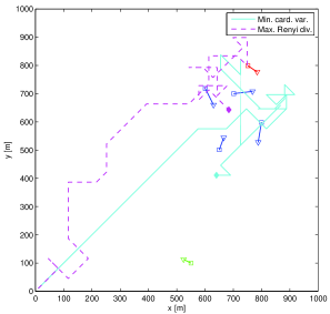
Figure 1: Typical sensor manoeuvres. Target start and stop positions are marked by $\square$ and $\nabla$, respectively. The red target died at $k=19$ while the green target was born at $k=27$.

We proceed to illustrate and compare the performance of the Rényi divergence and cardinality variance based sensor control strategies. In the case of the Rényi divergence, the implementation shown in Algorithm 2 is used to demonstrate the proposed CB-MeMBer filter based approach. For comparison, two PHD filter based algorithms are employed. The first approach uses a standard SMC implementation, which performs state estimation through k-means clustering. The second approach, as proposed in [13] sidesteps clustering with measurement driven state estimation techniques. In the case of the cardinality variance based control strategies, the two implementations shown in Algorithm 3 and 4 are trialled and compared. All algorithms were implemented in MATLAB R2010b on a laptop with an Intel Core i5-3360 CPU and 8GB of RAM. The average run time for the Rényi divergence based strategies are 0.99 seconds (CB-MeMBer), 2.46 seconds (PHD without clustering), and 2.51 seconds (PHD with $k$-means clustering) while those for cardinality variance based strategies are 0.61 seconds (non sampling) and 41.35 seconds (with sampling). As expected, the non sampling CB-MeMBer based strategy is the fastest.

Fig. 2 shows the averaged Optimal SubPattern Assignment (OSPA) metric [14] (with parameters $p=2$, $c=100m$) over 200 Monte Carlo runs for different control strategies. The OSPA curves in Fig. 2a suggest that the performance of PHD based strategies relies heavily on the partitioning of the particle population. While k-means clustering is highly unreliable, the measurement driven estimation [13] is more consistent. Furthermore, using the same Rényi divergence objective function, the CB-MeMBer filter based strategy outperforms the PHD filter based counterparts in terms of miss distance by approximate 10m in steady state. On the other hand, among CB-MeMBer based strategies, the OSPA curves of the cardinality variance based approaches decrease faster than that of the Rényi divergence based counterpart and are marginally lower in steady state as shown in Fig. 2b. This is because the cardinality variance based control strategies tend to drive the sensor more quickly towards targets which are initially present and tend to respond more sensitively to the birth of new targets. In contrast the Rényi divergence based control strategies tend to favour existing targets as they are on average more informative in terms of the objective function. As expected however, among the cardinality variance based approaches, the computational savings realized by the non sampling approach incur a slightly higher estimation error. To sum up, the results of Figure 2 indicate that, if the sensor obtains sufficient information on the target states, all CB-MeMBer based control strategies are effective and outperform the PHD based counterparts.

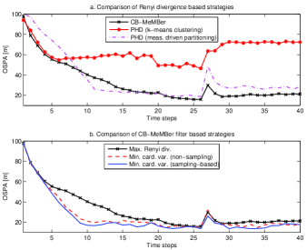
Figure 2: Comparison of OSPA by different methods (range bearing)

We now present a pathological example where the performance of the sensor control algorithm deteriorates significantly. Instead of bearings and range measurements, we now consider range only measurements and assume no target birth or death. It is expected that both the Rényi divergence and cardinality variance based strategies would both perform worse, since the range only measurements are much less informative, and actually result in a lower target “observability”. The single-object measurement model is now given by $g(\mathbf{z}|\mathbf{x};\mathbf{s})=\mathcal{N}(\mathbf{z};\|\mathbf{p}-\mathbf{s}\|,\sigma_{\zeta}^{2})$. Clutter is modelled by a Poisson RFS with intensity $\kappa(\mathbf{z})=\lambda\cdot c(\mathbf{z})$ with $c(\mathbf{z})=\mathcal{U(}\mathbf{z};[0,R_{\text{max}}])$. All other parameters are the same as those in the previous scenario.

Fig. 3 shows the averaged OSPA distance (with parameters $p=2$, $c=100m$) corresponding to the two objective functions after 200 Monte Carlo runs. It is clear that the Rényi divergence based strategy performs better, although neither control strategy achieves a sufficiently low OSPA error. The under-performance of both strategies can be explained by the lack of observability of the full states, as we now have range-only measurements. Minimizing the cardinality variance tends to drive the observer to a position where all the targets have roughly the same range so that the sensor can detect each of the targets equally well. However for range only sensors, this results in difficulty resolving the targets. On the other hand, an information theoretic criterion such as the Rényi divergence tends to account for both localization and cardinality criteria (albeit indirectly), and at least in this particular scenario, results in a different control policy with a lower error. Thus the “observability” of the targets is clearly a factor in determining the estimation performance of a particular control policy in different scenarios. Further work is required to investigate the notion of “observability” in a multi-target situation, and to develop a deeper understanding of what types of control policies are appropriate for different scenarios.

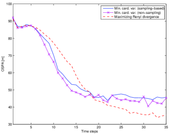
Figure 3: Comparison of OSPA by different methods (range only)

6 Conclusions and future works

The paper has presented a computationally tractable solution to the multi-target sensor management problem by combining POMDP theory with RFS or FISST based modelling. The CB-MeMBer filter was used to efficiently but approximately propagate a parametrized representation of the multi-object posterior density, which was then used to calculate a reward function in order to determine the action of the sensor. Using the particle CB-MeMBer filter not only allowed a conventional reward function, such as the Rényi divergence, to be calculated efficiently, but also enabled the estimated cardinality variance, which admits an analytic solution and provides direct control of cardinality estimation error, to be used as an objective function. In the latter case, a computationally fast control algorithm that does not require state space sampling has further been proposed. Numerical examples were presented, showing that when the sensor measurements are reasonably informative, with a high “observability” of the targets, both proposed control strategies work well. However, in pathological cases where there is low “observability” of targets, even though performance of both control policies degrades, the decrease in performance is noticeably worse for the cardinality variance based approach compared to the Rényi divergence based approach. Thus the “observability” of the targets is clearly a factor in determining the performance of a particular control policy in different scenarios. Further work is required to investigate the notion of “observability” in a multi-target situation, and to develop a deeper understanding of what types of control policies are appropriate for different scenarios.

References

- [1] D. A. Castanón and L. Carin. Stochastic control theory for sensor management. In A. O. Hero, D. A. Castanón, D. Cochran, and K. Kastella, editors, Foundations and Applications of Sensor Management, chapter 2, pages 7–32. Springer, 2008.
- [2] D. Daley and D. Vere-Jones. An introduction to the theory of point processes. Springer-Verlag, 1988.
- [3] A. Doucet, B.-N. Vo, C. Andrieu, and M. Davy. Particle filtering for multi-target tracking and sensor management. In Proc. 5th Annual Conference on Information Fusion (FUSION 2002), volume 1, pages 474–481, Annapolis Maryland, 2002.
- [4] A. O. Hero, C. M. Kreucher, and D. Blatt. Information theoretic approaches to sensor management. In A. O. Hero, D. A. Castanón, D. Cochran, and K. Kastella, editors, Foundations and applications of sensor management, chapter 3, pages 33–57. Springer, 2008.
- [5] H. G. Hoang. Control of a mobile sensor for multi-target tracking using Multi-Target/Object Multi-Bernoulli filter. In Proc. International Conference on Control, Automation and Information Sciences (ICCAIS 2012), pages 7–12, Ho Chi Minh City, Vietnam, 2012.
- [6] R. Mahler. Multi-target Bayes filtering via first-order multi-target moments. IEEE Trans. Aerosp. Electron. Syst., 39(4):1152–1178, 2003.
- [7] R. Mahler. Objective functions for Bayesian control-theoretic sensor management, I: Multitarget first-moment approximation. In Proc. IEEE Aerospace Conference, volume 4, pages 1905–1923, 2003.
- [8] R. Mahler. Multitarget sensor management of dispersed mobile sensors. In D. Grundel, R. Murphey, and P. Pardalos, editors, Theory and algorithms for cooperative systems, chapter 12, pages 239–310. World Scientific Books, 2004.
- [9] R. Mahler. PHD filters of higher order in target number. IEEE Trans. Aerosp. Electron. Syst., 43(4):1523–1543, 2007.
- [10] R. Mahler. Statistical Multisource-Multitarget Information Fusion. Artech House, 2007.
- [11] B. Ristic, S. Arulampalam, and N. Gordon. Beyond the Kalman filter: Particle filters for tracking applications. Artech House, 2004.
- [12] B. Ristic and B-N. Vo. Sensor control for multi-object state-space estimation using random finite sets. Automatica, 46(11):1812–1818, 2010.
- [13] B. Ristic, B-N. Vo, and D. Clark. A note on the reward function for PHD filters with sensor control. IEEE Trans. Aerosp. Electron. Syst., 47(2):1521–1529, 2011.
- [14] D. Schumacher, B-T. Vo, and B.-N. Vo. A consistent metric for performance evaluation of multi-object filters. IEEE Trans. Signal Process., 56(8):3447–3457, 2008.
- [15] S. Singh, N. Kantas, B.-N. Vo, A. Doucet, and R. Evans. Simulation based optimal sensor scheduling with application to observer trajectory planning. Automatica, 43(5):817–830, 2007.
- [16] D. Stoyan, D. Kendall, and J. Mecke. Stochastic Geometry and its Applications. John Wiley & Sons, 1995.
- [17] B.-N. Vo and W.-K. Ma. The Gaussian mixture probability hypothesis density filter. IEEE Trans. Signal Process., 54(11):4091–4104, 2006.
- [18] B.-N. Vo, S. Singh, and A. Doucet. Sequential Monte Carlo methods for multi-target filtering with random finite sets. IEEE Trans. Aerosp. Electron. Syst., 41(4):1224–1245, 2005.
- [19] B.-T. Vo, B.-N. Vo, and A. Cantoni. Analytic implementations of the cardinalized probability hypothesis density filter. IEEE Trans. Signal Process., 55(7):3553–3567, 2007.
- [20] B.-T. Vo, B.-N. Vo, and A. Cantoni. The cardinality balanced Multi-Target Multi-Bernoulli filter and its implementations. IEEE Trans. Signal Process., 57(2):409–423, 2009.