The Kardar-Parisi-Zhang equation with spatially correlated noise: a unified picture from nonperturbative renormalization group
Abstract
We investigate the scaling regimes of the Kardar-Parisi-Zhang equation in the presence of spatially correlated noise with power law decay in Fourier space, using a nonperturbative renormalization group approach. We determine the full phase diagram of the system as a function of and the dimension . In addition to the weak-coupling part of the diagram, which agrees with the results from Refs. [Europhys. Lett. 47, 14 (1999), Eur. Phys. J. B 9, 491 (1999)], we find the two fixed points describing the short-range (SR) and long-range (LR) dominated strong-coupling phases. In contrast with a suggestion in the references cited above, we show that, for all values of , there exists a unique strong-coupling SR fixed point that can be continuously followed as a function of . We show in particular that the existence and the behavior of the LR fixed point do not provide any hint for 4 being the upper critical dimension of the KPZ equation with SR noise.
pacs:
05.10.Cc,64.60.Ht,68.35.Ct,68.35.RhI Introduction
To describe interface roughening and its dynamical scaling, Kardar, Parisi and Zhang (KPZ) proposed a nonlinear Langevin equation, which has now emerged as a fundamental model to study nonequilibrium phase transitions and scaling phenomena Kardar et al. (1986); Halpin-Healy and Zhang (1995); Krug (1997); Barabási and Stanley. (1995). The KPZ equation Kardar et al. (1986) writes
| (1) |
where is a single valued height profile which depends on the -dimensional spatial coordinate of the substrate and on time , the surface tension, and represents a Gaussian noise with zero mean and variance
| (2) |
The non-linear term proportional to is the essential ingredient to capture the dynamical roughening of the interface Halpin-Healy and Zhang (1995); Krug (1997); Barabási and Stanley. (1995).
The original KPZ equation is formulated with a purely local noise of amplitude , that is . This equation encompasses the following behavior. It always generates scaling in the stationary regime, characterized by the dynamical and the roughness critical exponents. For dimensions , the interface always roughens, whereas for , a nonequilibrium phase transition occurs for a critical value of the non-linearity, which separates a strong-coupling () rough phase from a weak-coupling () smooth phase corresponding to the linear Edwards Wilkinson (EW) regime, with exponents and . The ubiquity of the KPZ universality class has led to considerable efforts over the last decades to understand its statistical properties Halpin-Healy and Zhang (1995); Krug (1997). We do not review here all the corresponding literature, but only mention the most recent contributions. For one-dimensional interfaces, an impressive breakthrough has been achieved during the last years both theoretically Prähofer and Spohn (2004); Sasamoto (2005); Sasamoto and Spohn (2010); Calabrese and Le Doussal (2011); Amir et al. (2011); Imamura and Sasamoto (2012) (and for a review, see e.g. Corwin (2012)) and experimentally Takeuchi and Sano (2010); Takeuchi et al. (2011); Takeuchi and Sano (2012). For higher-dimensional interfaces, recent large scale numerical simulations were launched to refine the estimates of critical exponents and probability distributions Kelling and Ódor (2011); Pagnani and Parisi (2013); Halpin-Healy (2012, 2013a); *Halpin-Healy13err; Oliveira et al. (2013). However, the progress is much slower, leaving still unsettled debates such as the existence of an upper critical dimension for this model.
Recently, we proposed a nonperturbative renormalization group (NPRG) approach for the KPZ equation Canet et al. (2010, 2011a); *Canet12Err; Kloss et al. (2012), which successfully yielded the fully attractive (short-range (SR)) strong coupling fixed point describing the rough phase in all dimensions. The associated exponents are in close (resp. reasonable) agreement in (resp. ) with the estimates from numerical simulations Tang et al. (1992); Ala-Nissila et al. (1993); Castellano et al. (1999); Marinari et al. (2000); Aarão Reis (2004); Ghaisas (2006); Kelling and Ódor (2011); Pagnani and Parisi (2013). The finding of the fully attractive strong-coupling fixed-point allows one to show the emergence of generic scaling for the 2-point correlation and response functions. The resulting scaling functions in compare remarkably well with the exact results Canet et al. (2011a); *Canet12Err; Prähofer and Spohn (2004). These calculations have been extended in any dimensions, giving in particular the 2-point correlation and response functions in and Kloss et al. (2012). The ensuing predictions for the associated universal amplitude ratios in have been recently accurately confirmed in lattice simulations Halpin-Healy (2013a).
We here address the issue of the presence of long-range (LR) correlated noise in the KPZ equation. Some experimental realizations (such as wetting in porous media Rubio et al. (1989); Horvath et al. (1991)) suggested that spatial correlations may exist at the microscopic level, in the noise or in the hydrodynamical interactions Halpin-Healy and Zhang (1995); Krug (1997); Barabási and Stanley. (1995). This has triggered the study of the relevance of this type of microscopic correlations, as for its impact on the critical exponents and on the phase diagram. Several numerical and theoretical studies have shown that spatial Meakin and Jullien (1989); Hentschel and Family (1991); Amar et al. (1991); Peng et al. (1991); Pang et al. (1995); Li (1997); Mukherji and Bhattacharjee (1997); Janssen et al. (1999); Frey et al. (1999); Katzav and Schwartz (1999); Verma (2000); Katzav (2003, 2013) and/or temporal Medina et al. (1989); Lam et al. (1992); Katzav and Schwartz (2004); Fedorenko (2008) noise correlations indeed lead to new phases with modified exponents. Following Ref. Medina et al. (1989); Janssen et al. (1999); Frey et al. (1999); Katzav and Schwartz (1999), we consider, in addition to the local delta-correlated SR noise, a spatially correlated noise of the form
| (3) |
More precisely, the full noise term writes in Fourier space
| (4) |
where and is the relative amplitude of the LR noise.
The early dynamical renormalization group (DRG) analysis by Medina et al. Medina et al. (1989) predicted the existence of a rough LR dominated phase above a threshold value of the decay exponent of the LR noise, with associated -dependent critical exponents and . This prediction was confirmed by a functional RG calulcation for directed polymers Halpin-Healy (1990). Yet some other theoretical approaches, based on a replica scaling analysis Zhang (1990) or on a scaling analysis in open dissipative systems Hentschel and Family (1991) yielded alternative predictions for the critical exponents and the threshold value of . As early numerical simulations, mainly in one dimension, were not in accordance, the situation was unclear. However, later simulations Hayot and Jayaprakash (1996) of the Burgers equation in clearly confirmed the original DRG results, which were then also supported by a Mode-Coupling calculation Bhattacharjee (1998), a Self-Consistent Expansion Katzav and Schwartz (1999); Katzav (2013) (at least in ), and exact results from a DRG calculation using a stochastic Cole-Hopf transformation by Janssen, Frey, and Täuber (JFT) Janssen et al. (1999); Frey et al. (1999). We present below the findings of JFT, which will serve as a reference for later comparison with our work.
JFT have shown that, in the presence of LR noise, new LR dominated weak-coupling phases exist. They also suggested the existence of a LR dominated strong coupling phase even if the perturbative analysis cannot find the associated fixed point. Furthermore, they derived exact (i.e. valid to all orders in perturbation theory) expressions for the corresponding -dependent exponents, including the LR dominated strong-coupling phase (under the assumption that the associated fixed-point exists), which coincide with the DRG one-loop result. The physical picture emerging from their work is as follows. Below a lower critical dimension , no smooth phase is stable, that is, the interface is always rough and the LR noise is either irrelevant at moderate () or dominates at larger (). The computation of is not accessible perturbatively, but is approximated by JFT by a linear interpolation between the exact result and the point , deduced from a mapping to the Burgers equation with non-conserved noise (however, see below). Above , the two phases, smooth and rough, exist and JFT find that the LR noise is always relevant in the smooth phase while it is always irrelevant in the rough phase. From their results, they infer that the upper critical dimensions of the roughening transition and of the SR rough phase below are . JFT also conjecture that the SR rough phases above and below may be of two different natures (called SR-I and SR-II in their paper), with possibly different upper critical dimensions Janssen et al. (1999); Frey et al. (1999).
In the present paper, we revisit the work by JFT using the nonperturbative renormalization group (NPRG) approach, successfully developed for the (SR noise) KPZ equation Canet et al. (2010, 2011a); *Canet12Err; Kloss et al. (2012), and here generalized to include Gaussian LR correlated noise. We derive the corresponding NPRG flow equations at the Next-to-Leading Order (NLO) approximation of Ref. Kloss et al. (2012), and solve them to determine the full phase diagram of the system for various values of and . Our results are in close agreement with the results of JFT in the weak-coupling sector. We recover in particular the smooth LR phases predicted above with their exact critical exponents and correction-to-scaling exponents. Furthermore, we find the two stable fixed point solutions in the strong-coupling regime (in their respective existence domain), describing the SR and the LR rough phases, with the exact LR exponents, and we compute the stability boundary line . The obtention of the complete phase diagram of the system in the plane with all the expected fixed points constitutes our main result. In particular, we find that there exists a unique strong-coupling fixed-point describing the SR rough phase in all dimensions, which is not consistent with the conjecture by JFT of the existence of two different rough phases SR-I and SR-II above and below . Furthermore, we investigate the phase diagram in the strong-coupling regime around , at least qualitatively since the NLO approximation is no longer accurate in this regime for . Combining our findings and critical exponents from numerical simulations Ala-Nissila et al. (1993); Castellano et al. (1998, 1999); Marinari et al. (2000); Pagnani and Parisi (2013), we argue that may not necessarily be the upper critical dimension of the SR rough phase. However, as the value of the SR roughness exponent in cannot be reliably determined at this level of approximation, we cannot conclude yet about the actual value of within NPRG, which requires a higher order approximation and is left for future investigation.
The remainder of the paper is organized as follows. In Sec. II, we briefly present the NPRG formalism for the KPZ equation, including LR correlated Gaussian noise, and the approximations used. We then derive the corresponding flow equations. These equations are numerically integrated in Sec. III, and the full phase diagram of the system is determined and presented, including a discussion about the upper critical dimension.
II Nonperturbative renormalization group
II.1 KPZ field theory and symmetries
The field theory associated with the KPZ equation (1) with both SR noise and Gaussian LR correlated noise is derived in Ref. Janssen et al. (1999), following the Janssen-de Dominicis procedure Janssen (1976); *dominicis76. The KPZ dynamic generating functional is given by
| (5a) | ||||
| (5b) | ||||
where is the Martin-Siggia-Rose response field Martin et al. (1973), and are sources, and the notation , was introduced.
The symmetries of the KPZ action with correlated noise are two-fold: (i) the -shift symmetry, (ii) the Galilean symmetry. The additional discrete time reversal symmetry of the one-dimensional SR KPZ equation is no longer realized in presence of correlated noise. Moreover, as in the SR KPZ case, the symmetries (i) and (ii) are gauged in time Canet et al. (2011a); Lebedev and L’vov (1994) and correspond to the following infinitesimal field transformations:
| (i) | (6c) | ||||
| (ii) | (6d) | ||||
where and are arbitrary infinitesimal time dependent quantities. The variations of the KPZ action (5b) under these time-gauged transformations are linear in the fields, and thus entail simple Ward identities, with a stronger content than the usual non-gauged ones Canet et al. (2011a). The detailed analysis of these symmetries is at the heart of the construction of the NPRG approximation scheme, derived in Canet et al. (2011a).
II.2 NPRG formalism
The general NPRG formalism for nonequilibrium systems is presented in Ref. Canet et al. (2011b); Berges and Mesterházy (2012); Kopietz et al. (2010), and its specific application to the KPZ equation in Ref. Canet et al. (2011a). We only recall here the main elements, following Ref. Canet et al. (2011a). In the spirit of Wilson’s RG ideas, the NPRG formalism consists in building a sequence of scale-dependent effective models such that fluctuations are smoothly averaged as the (momentum) scale is lowered from the microscopic scale , where no fluctuations are yet included, to the macroscopic scale , where they are all summed over Berges et al. (2002); Delamotte and Canet (2005). For classical nonequilibrium problems, one formally proceeds as in equilibrium, but with the presence of the response field, and additional requirements stemming from It’s discretization and causality issues Canet et al. (2011b); Benitez and Wschebor (2012).
To achieve the separation of fluctuation modes within the NPRG procedure, one adds to the original action a momentum and scale dependent mass-like term:
| (7) |
where the indices label the field and response field, respectively , and summation over repeated indices is implicit. The matrix elements are proportional to a cutoff function , with , which ensures the selection of fluctuation modes: is required to almost vanish for such that the fluctuation modes are unaffected by , and to be large when such that the other modes () are essentially frozen. Furthermore, must preserve all the symmetries of the problem and causality properties. As advocated in Canet et al. (2011a), an appropriate choice is
| (8) |
where the running coefficients and , defined later (Eq. (17)), are introduced in the regulator for convenience Canet et al. (2010). Here we choose the cutoff function
| (9) |
The dependence of our results on the parameter is discussed in Appendix B.
In the presence of the mass term , the generating functional (5a) becomes scale dependent
| (10) |
Field expectation values in the presence of the external sources and are obtained from the functional as
| (11) |
The effective action is defined as the Legendre transform of (up to a term proportional to ) Berges et al. (2002); Delamotte (2012); *delamotte07; Canet et al. (2011b):
| (12) |
The exact flow for is given by Wetterich’s equation, which writes in Fourier space Wetterich (1993); Berges et al. (2002)
| (13) |
where
| (14) |
is the full, that is, field-dependent, renormalized propagator of the theory. When is lowered from to 0, interpolates between the microscopic model and the full effective action that encompasses all the macroscopic properties of the system Canet et al. (2011b). Of course Eq. (13) cannot be solved exactly, one has to resort to an appropriate approximation scheme, adapted to the specific model under study, and in particular to its symmetries.
II.3 Approximations
II.3.1 Next-to-Leading Order (NLO) approximation
In Ref. Canet et al. (2011a), inspired by the previous work in equilibrium statistical mechanics of Refs. Blaizot et al. (2006); Benitez et al. (2009, 2012), an approximation scheme is devised, which consists in building an ansatz for explicitly preserving the gauged shift (6d) and gauged Galilean (6c) symmetries. The building blocks are the Galilean invariants , , the covariant time derivative , combined with the operators and . We work here in the rescaled theory where and . Within this scheme, the ‘second order’ (SO) ansatz for writes
| (15) |
where , are three running functions. It is a truncation at quadratic order in the response field , while the complete momentum and frequency dependence of the 2-point functions is preserved. Note that infinite powers of the field itself are included through the covariant time derivatives . At the bare level , and for purely local noise, one has ,
The SO flow equations for the functions , derived in Canet et al. (2011a), were integrated in the simpler one-dimensional case, where the additional time reversal symmetry imposes that there remains only one independent running function. The scaling functions associated with the 2-point correlation function were computed, and showed an impressive agreement with the exact results Canet et al. (2011a); Prähofer and Spohn (2004). However, the integration of the SO flow equations in generic dimensions appears rather involved, and a further simplification was proposed in Kloss et al. (2012). This approximation, referred to as NLO, consists in neglecting the frequency dependence of the three flowing functions within the loop integrals, that is, the right hand side of the flow equations. The NLO flow equations can be found in Kloss et al. (2012), where they were integrated in and and the scaling functions associated with the 2-point correlation and response functions were computed. The related prediction for a universal amplitude ratio in was very recently confirmed with great accuracy in lattice simulations Halpin-Healy (2013a).
In the present paper, we work with LR noise at the NLO approximation. Moreover, we focus on zero external frequency, since we are merely interested in the phase diagram and in the critical exponents, and not in the full scaling functions. The zero-frequency sector is decoupled from the non-vanishing frequency sector within the NLO approximation, and we denote for simplicity. The inclusion of the noise Eq. (4) then simply amounts to the substitution
| (16) |
(with bare condition ) in the NLO ansatz. The first term corresponds to the renormalized SR contribution at scale , and the second term to the LR one. This separation in terms of a regular () and a nonanalytic part () holds for any because, as the flow is regularized in the IR and finite in the UV, it cannot generate nonanalytic contributions. Correspondingly, the nonanalytic part is not renormalized () and the coupling remains equal to its bare value. Thus, in the presence of LR noise, the NLO flow equations for the three functions are identical to those for the local SR case, up to the substitution (16).
The gauged shift symmetry implies the non-renormalization of that therefore remains equal to unity for all . Moreover, the Galilean symmetry implies the non-renormalization of the non-linear coupling . We hence define two scale dependent parameters and
| (17) |
These two running coefficients yield two running anomalous dimensions, defined according to
| (18) |
which fixed point values, indexed by *, are related to the physical critical exponents by
| (19) |
In order to study fixed point properties, we introduce dimensionless quantities. The dimensionless couplings are
| (20a) | ||||
| (20b) | ||||
and their flow equations, due to the non-renormalization of and , are hence reduced to their dimensional parts
| (21a) | ||||
| (21b) | ||||
with . The dimensionless running functions are defined by
| (22) |
for and , and their flows write
| (23) |
with , , and the are the loop integrals, which explicit expressions are given in Ref. Kloss et al. (2012), up to the substitution (16).
The five flow equations (21,23) are solved numerically with Euler time stepping and in the RG “time” . The three flowing functions are set to unity at the initial scale . We observe that the flow always converges to a stable fixed point, which nature depends on the initial conditions for and . From these flows, one then deduces the phase diagram in the plane for each value of the parameters , which is discussed in Sec. III.
II.3.2 Local potential approximation
As studied in detail in Ref. Kloss et al. (2012), the NLO approximation gives a reliable quantitative description of the SR fixed point up to 3.5. However, the numerical cost to solve the coupled NPRG flow equations is high, especially as the flow, in the vicinity of unstable fixed points, slows down to impractical timescale. To fully explore the phase diagram, it is therefore convenient to sometimes resort to an additional approximation, usually referred to as the Local Potential Approximation prime (LPA’) Delamotte (2012) where only field-independent renormalization coefficients are kept. It thus consists in the following simplification:
| (24) |
The LPA’ was shown to already capture the qualitative structure of the phase diagram in the pure SR case, although the estimate for the critical exponents rapidly deteriorates as the dimension grows Canet (2005). This approximation will be used to determine the weak-coupling part of the phase diagram. The complete NLO approximation is however necessary to study the boundary between the SR and LR dominated rough phases in 2 and 3. It indeed turns out that the value of the roughness exponent is overestimated at the LPA’, such that the stability change of the SR and LR fixed points is shifted to unphysical values where in this approximation, see Eq. (3). In the following, we will indicate whether the NLO or the LPA’ is used.
II.4 Change of variables
As found by JFT, the LR weak-coupling fixed points (EWLR1 and EWLR2, see below) describing the smooth phase when it exists have an infinite noise amplitude coordinate . It is therefore convenient to change variables such that the fixed point coordinates remain finite. We choose the same variables as JFT Janssen et al. (1999); Frey et al. (1999), namely
| (25) |
to simplify the comparison.
In terms of the new couplings and , the flow equations (21) become
| (26a) | ||||
| (26b) | ||||
where we have implicitly assumed that the anomalous dimensions , which depend on and , are now expressed in terms of and .
III Results
III.1 Fixed points
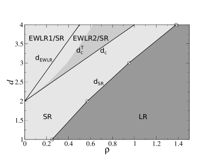
We study in the following the existence and stability of the fixed point solutions of the NPRG flow equations (26,23) as functions of and . Three fixed points correspond to a vanishing and are thus referred to as Edwards-Wilkinson fixed points. One (denoted EW) is at while two others (EWLR1 and EWLR2) correspond to infinite , that is, . Another fixed point, denoted T (for transition) exists at and (for ) and separates at vanishing LR noise amplitude the smooth and rough phases. All these four fixed points were found perturbatively and their coordinates, stability and associated exponents were obtained exactly in the Cole-Hopf representation of the theory Janssen et al. (1999). Besides these fixed points, we find three others. Two, denoted SR and LR, describe the rough phase, respectively when the LR noise is irrelevant and relevant. These fixed points are genuinely nonperturbative, that is, are not accessible at any order of the perturbative expansion. The last fixed point, denoted TLR (for transition in the presence of LR noise), exists in a (narrow) band of the plane that separates, above the band, a region where there exists a transition between the smooth and rough phases, and below the band, a region where there is no stable smooth phase and where the long distance physics is described by either SR or LR (when, initially, the amplitude of the noise is nonvanishing).
III.1.1 Edwards-Wilkinson fixed point
The EW fixed point corresponds to which implies and . This fixed point is always unstable with respect to LR noise, i.e. in the direction. It is repulsive (resp. attractive) in the (or ) direction for (resp. ).
III.1.2 EWLR1 fixed point
This fixed point is located at . It is always attractive in the -direction while it is attractive (resp. repulsive) for (resp. for ) in the -direction, see the Appendix A. At this fixed point, , and the exponents are and . The associated correction-to-scaling exponents are and , see Appendix A.
III.1.3 EWLR2 fixed point
The EWLR2 fixed point exists for (it coincides with EWLR1 at ) and is located at and , see Eq. (A18). It is always attractive in the -direction, while its stability in the -direction changes at , from unstable for to stable for . The critical exponents and are identical in the two LR smooth phases. However, as already emphasized by JFT, they differ by their correction-to-scaling exponents, which are for EWLR2 and , see Appendix A.
III.1.4 Transition fixed point
The transition fixed point T exists for at and (it coincides with EW in ). It is always unstable in the -direction. In the Cole-Hopf representation, the change of stability of T in the -direction occurs exactly at (or equivalently at ), simultaneously with the change of stability of EWLR2, via the appearance of a line of fixed points joining the two fixed points Janssen et al. (1999). Within our approximations, we find, at fixed , that T is stable in the -direction at small and that its stability changes at (or equivalently at ) since the exact value for the critical exponent at the transition is only recovered approximately within our approximations. (Given that NLO and LPA’ are exact at one loop, we find, as expected . However, when grows, it becomes slightly negative rather than strictly vanishing).
III.1.5 TLR fixed point
This fixed point is found for (equivalently, for ) and has coordinates and . It is unstable in the -direction and drives the transition between SR and EWLR2. As explained above, in the Cole-Hopf representation, the stabilities of the two fixed points T and EWLR2 are switched together through the appearance at of a fixed line joining them. This feature is not preserved by our approximation. We find instead that at fixed and upon increasing , the TLR fixed point first crosses T at , then travels up the entire plane , before eventually crossing EWLR2 at . The line of fixed points is thus replaced by the TLR fixed point which moves very rapidly between T and EWLR2 as is increased. This feature is probably an artifact of our approximations (if the line of fixed points is an exact result, valid beyond perturbation theory). However, the flow is modified only in a narrow band between and , and the physically observable phases remain unaffected, controlled by the fully attractive EWLR2 or SR fixed point (compare Figs. 3 and 4).
III.1.6 Short-range fixed point
The SR fixed point is located and . It exists in all dimensions and describes the rough (strong-coupling) phase of the KPZ equation without LR noise. Within all our approximations (except the LPA’), the associated exponents are in good agreement with the numerical ones in and Canet et al. (2010, 2011a); *Canet12Err; Kloss et al. (2012). The quality of our approximations deteriorates with increasing dimension and none of them yields reliable quantitative results above typically . In all dimensions we find that SR is stable in the -direction. Its stability in the noise direction can be inferred from Eq. (19) and Eq. (26), that is
| (27) |
The sign change of the -function in the -direction hence occurs at
| (28) |
At fixed , the SR fixed point is attractive in the noise direction for and becomes repulsive beyond this value.
III.1.7 Long-range fixed point
The LR fixed point has coordinates and and describes a strong-coupling rough, LR dominated phase. At fixed , it exists for (it coincides with SR at ) and is attractive in all directions. Under the assumption that it indeed exists, the associated exponents have been determined exactly in the Cole-Hopf representation Janssen et al. (1999):
| (29) |
and are also obtained exactly from the NPRG Eqs. (19,21) at any non-trivial fixed point with nonvanishing LR noise. Let us notice that the LPA’ is not sufficient to find with a reasonable accuracy the value of where SR and LR exchange their stability and we resorted to the complete NLO approximation to get it. We compare in Table 1 the location of the boundary line between the SR and LR phases obtained with different approaches. The JFT result corresponds to a linear interpolation proposed by these authors Janssen et al. (1999). The NLO and the numerical results correspond to the value of verifying , that is , where the values for are obtained respectively from the NLO approximation or numerical simulations Tang et al. (1992); Ala-Nissila et al. (1993); Castellano et al. (1999); Marinari et al. (2000); Aarão Reis (2004); Ghaisas (2006); Kelling and Ódor (2011); Pagnani and Parisi (2013).
| 1 | 2 | 3 | 4 | |
|---|---|---|---|---|
| 1/4 | 1/2 | 3/4 | 1 | |
| 1/4 | 0.57 | 0.79 | – | |
| 0.25 | 0.57 | 0.95 | 1.37 |
III.2 Discussion of the phase diagram
After having characterized all the fixed point solutions of the NPRG flow equations, we now provide a complete picture of the phase diagram (see Fig. 1). There are two distinct situations depending on the dimension. First we confirm the general picture found by JFT. That is, for , the interface is always rough, with a phase boundary separating the usual strong coupling SR phase for and a LR dominated phase with -dependent critical exponents for . Above , the T fixed point drives a transition between a smooth LR phase and a rough SR phase. In the following, we discuss the details of the phase diagram, reasoning rather at fixed and for varying , which is closer in spirit to what can be observed in simulations.
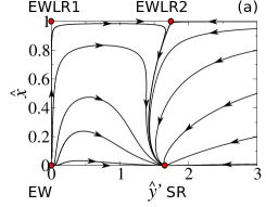
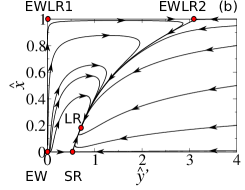
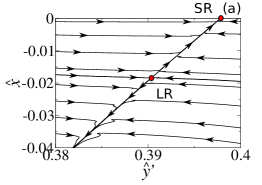
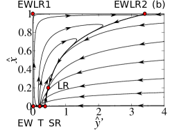
For , the system is always in a rough phase and for the flow is driven to the SR fixed point whatever the initial condition is, provided the nonlinearity is nonvanishing (), see Fig. 2 (a). In this case, the presence of the LR noise does not change the long distance physics of the KPZ equation. At , the LR fixed point crosses SR and enters the physical quadrant for . It is then fully attractive and drives the long distance physics of any model showing nonvanishing LR noise, see Fig. 2 (b).
For , the situation is more complex. At vanishing LR noise amplitude (), the fixed point T separates a smooth (at small ) and a rough (at large ) phase. The smooth phase is described by the usual EW fixed point and the rough phase by the SR fixed point. For and nonvanishing noise amplitudes, there exists a critical line (highlighted in blue in Figs. 3 and 4) ending at T also separating a smooth and a rough phase. This line is nontrivial as can be seen on the panels (a) to (c) of Fig. 3. Depending on , the flow in the smooth phase is either driven, for to EWLR1, Fig. 3 (a), or for to EWLR2, Fig. 3 (b). In the rough phase, the flow is driven to SR for , Figs. 3 (a) to (d), which becomes fully attractive in the entire plane for , Figs. 3 (d). In this case, the LR noise is irrelevant and the LR fixed point lies in the unphysical quadrant . For , the LR fixed point crosses SR and appears in the physical quadrant becoming the dominant, fully attractive fixed point Fig. 3 (e). For and , the flow is thus very similar to what is found in : either and SR is fully attractive or and LR is fully attractive and governs the rough phase. Let us emphasize that we can follow continuously all these fixed points in the plane and that there are no two distinct SR phases contrary to what was conjectured in Janssen et al. (1999).
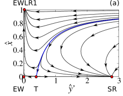
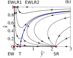
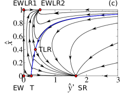
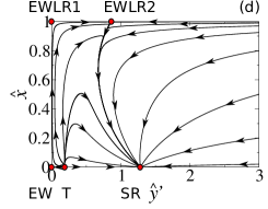
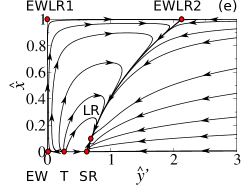
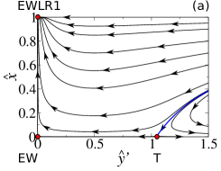
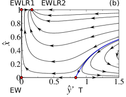
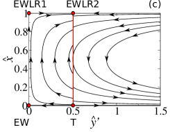
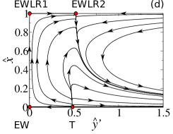
As already mentioned, if no approximation were performed and in the perturbative Cole-Hopf approach, a fixed line joining T to EWLR2 would appear exactly at and for both fixed points would become unstable, see Fig. 4. Instead, within our approximations and upon increasing at fixed , the unstable fixed point TLR crosses T for , moves very rapidly towards EWLR2 and finally crosses this fixed point at , Fig. 3 (c) and (d), changing the stability of these fixed points upon crossing them. However, this little discrepancy does not modify qualitatively the rest of the phase diagram and the physically observable phases are unaffected (compare Figs. 3 and 4).
III.3 Discussion about the upper critical dimension
We have followed the LR fixed point up to dimension 4 for 111In , we choose the cutoff parameter , see Appendix B.. We observed that it does not lie close to the Gaussian fixed point near and . In fact, within the NLO approximation, we find in that a transition between the SR and LR dominated phases occurs at , such that the LR fixed point becomes the stable fixed point for with a finite value of , see Fig. 5. We recall that our results in the strong coupling phase show a large dependence on the choice of regulators for dimensions larger than typically 3.5, which strongly suggests that our approximations are not accurate in this case, see Appendix B. However, there is no doubt that the LR fixed point cannot become Gaussian in and . As a matter of fact, if it were Gaussian, it would exist as a solution of the perturbative expansion of our NPRG equations since our approximations, either the LPA’ or NLO, are exact at one-loop order by construction. There is no such a solution. Put it differently, while the strong coupling regime of the problem becomes out of reach of our approximations in large dimensions, the weak coupling regime remains under control. In the NPRG calculations, the case and does not map onto the Burgers equation with non-conserved noise, (i.e. model B of Forster et al. Forster et al. (1977) applied to the Burgers equation). In the latter, only a LR noise is present and it does not include a SR part, such that nothing can be inferred from this model about the stability of the LR fixed point against a SR component. The reason for the discrepancy with JFT who advocated this mapping is that, in the RG approach, the SR noise is generated by the flow even if it is not present initially and it cannot be neglected. The full complexity of the KPZ equation with both types of noise, and their competition, cannot be avoided to determine their respective relevance. As a result, the usual power counting argument performed in model B (for LR without a SR component) leading to an upper critical dimension of 4 for LR cannot be applied here.
Within the NPRG framework, as already mentioned, the NLO approximation is not accurate above 3.5. However, the qualitative structure of the obtained phase diagram in in the strong-coupling sector (Fig. 5), together with some inputs from numerical simulations for the critical exponent, open up another possibility, which we now stress. The stability exchange between SR and LR proceeds when LR comes across SR from below, which occurs for . Thus, if in , as suggested by numerical simulations, SR appears as the stable fixed point for , dominating over LR, which has and still lies in the unphysical quadrant of the coupling constant space (see Fig. 1). From simulation results for , the SR stability change in occurs around , and thus SR is still fully attractive at Ala-Nissila et al. (1993); Castellano et al. (1998, 1999); Marinari et al. (2000); Pagnani and Parisi (2013).
Let us summarize the previous discussions of the phase diagram and of . We emphasized that the existence of two different types of SR phases above and below with different upper critical dimensions is not consistent with our finding of a unique SR fixed point. However, we proposed an alternative scenario which could reconcile numerical simulations and RG analysis, namely that the LR fixed point is unstable against SR at and . Let us emphasize once more that we cannot settle yet whether this scenario is realized within NPRG, i.e. whether is vanishing or not in . Doing so requires a higher-order approximation, and this issue will be addressed in future work.
IV Conclusion
In the present work, we investigated, using NPRG, the phase diagram of the KPZ equation with Gaussian LR correlated noise with power law decaying correlator in Fourier space. We generalized the NPRG flow equations in the NLO approximation to include LR noise. We then integrated them numerically to determine the complete phase diagram of this model as a function of and , and confronted it with the results obtained by JFT, which are valid to all order in perturbation theory.
In the weak-coupling sector, the two approaches are in close agreement. We recover in particular that above , the smooth phase is LR dominated and is controlled by one of the two weak-coupling LR fixed points EWLR1 or EWLR2, with their exact critical exponents and correction-to-scaling exponents. One difference appears between the two approaches: the line of fixed point joining T and EWLR2 at exactly is replaced in the NPRG approach at NLO by an unstable fixed point TLR rapidly moving from T to EWLR2 as is increased in the vicinity of . This difference originates in the fact that the transition fixed point T is only approximately described within the NLO approximation. It has however a negligible impact on the structure of the phase diagram.
In the strong-coupling sector, we find the two fixed points that govern the SR and LR rough phases, which constitutes our main result. They exchange their stability when LR comes across SR from an unphysical quadrant of the coupling space which occurs for . We hence computed the phase boundary which is not accessible within perturbation theory. All of the fixed points can be followed continuously when and are varied, and we show in particular that there exists a unique SR fixed point. This is not consistent with the scenario proposed by JFT of two SR phases, below and above respectively, of different natures. We finally suggest that the RG finding does not in fact rule out the possibility that the SR phase (SR-I in JFT’s work) has an upper critical dimension different from 4, and possibly infinite, which would be compatible with the numerical results. However, the NLO approximation we used does not allow us to determine whether this possibility is realized within NPRG, as the NLO approximation does not allow us to accurately investigate the case. This is left for future work.
V Acknowledgments
The authors acknowledges financial support from the ECOS-Sud France-Uruguay program U11E01. TK thanks the LPTMC at the Université Pierre et Marie Curie for hospitality, where parts of this work were achieved. TK also gratefully acknowledges financial support from the Alexander von Humboldt foundation, the IIP in Natal and for hospitality and computing resources in the Group of P. Kopietz at the Goethe University Frankfurt. Finally, LC and BD thank the Universidad de la República (Uruguay) for hospitality and the PEDECIBA for financial support during the completion of this work.
Appendix A: perturbative analysis of NPRG equations
In this Appendix, we analyze the NPRG flow equations in some perturbative regimes. In the vicinity of and , the NPRG flow equations coincide with Eqs. (4.33,4.34) of Ref. Janssen et al. (1999), which read in our normalizations, that is with :
| (A1a) | ||||
| (A1b) | ||||
with .
The NPRG -functions for these couplings are given by Eqs. (21). The anomalous dimensions are defined at zero external momentum, through the normalization conditions ensuing from definitions (17,22). Eq. (23) then yields the implicit equation for the anomalous dimensions
| (A2) |
where both integrals and depend linearly on and . We hence define
| (A3a) | ||||
| (A3b) | ||||
The explicit form of the various integrals is given by Kloss et al. (2012):
| (A4a) | ||||
| (A4b) | ||||
| (A4c) | ||||
| (A4d) | ||||
| (A4e) | ||||
| (A4f) | ||||
where
| (A5a) | ||||
| (A5b) | ||||
[Note two misprints in Eqs. (A4d) and (A4f) of Ref. Kloss et al. (2012) corrected here].
To investigate the properties of the EWLR fixed points, we consider the limit and , at fixed, that is at fixed . As long as , and are of order one in this limit (which holds by definition at LPA’ and is verified below at NLO), it amounts to replacing in the various Eqs. (A4) by . Accordingly, one observes that
| (A6a) | ||||
| (A6b) | ||||
| (A6c) | ||||
| (A6d) | ||||
| (A6e) | ||||
| (A6f) | ||||
Let us check the behavior of the three functions in this limit in the NLO approximation. The NLO flow equations for the functions , and (see Kloss et al. (2012)) are of order
| (A7a) | ||||
| (A7b) | ||||
| (A7c) | ||||
As a consequence, in the limit at fixed , one has indeed
| (A8a) | ||||
| (A8b) | ||||
| (A8c) | ||||
Therefore, even if does not remain at bare level along the flow, the NLO and LPA’ expressions for the anomalous dimensions Eqs. (A2) in this limit are identical and become
| (A9) |
with
| (A10a) | ||||
| (A10b) | ||||
Moreover the perturbative expansion of the NPRG flow equations for the couplings Eqs. (A1) in the variables and become
| (A11a) | ||||
| (A11b) | ||||
To study the stability of the EWLR fixed points, these flow equations can be linearized in the vicinity of a fixed point with and the corresponding stability matrix reads
| (A13) | ||||
| (A16) |
To determine the component requires to push the expansion (A11) of to order , but this is not necessary for the study of the stability of fixed points with . The expression (A16) of the stability matrix implies that for any fixed point with , the two eigenvalues, which identify with the correction-to-scaling exponents, are and . We now discuss the two fixed point with .
EWLR1 fixed point
The EWLR1 fixed point is located at and . The corresponding correction-to-scaling exponents are
| (A17) |
that are identical to the correction-to-scaling exponents obtained by JFT Frey et al. (1999); Janssen et al. (1999). Consequently, we recover the same stability conditions, namely the EWLR1 fixed point is always attractive in the -direction, whereas it is attractive in the -direction for and repulsive for .
EWLR2 fixed point
The coordinates of the EWLR2 fixed point are
| (A18) |
and the corresponding correction-to-scaling exponents are given by
| (A19) |
which again identify with the correction-to-scaling exponents found perturbatively Frey et al. (1999); Janssen et al. (1999). Checking that is always positive, we deduce the same stability conditions as JFT. The EWLR2 fixed point is always attractive in the -direction, and EWLR1 and EWLR2 exchange their stability in the -direction when EWLR2 crosses EWLR1 at .
Appendix B: Cutoff dependence
In this Appendix, we discuss the dependence of our results in the regulator function, which can be tested via the variation of the (positive) parameter in Eq. (9). Of course, physical observables computed from the exact NPRG equation (13) do not depend on the choice of regulator. However, any approximation induces a spurious dependence in this regulator, which can be used to test the quality of the approximation.
The dependence of the critical exponent of the SR fixed point at the NLO approximation has been studied in details in Ref. Kloss et al. (2012). The exponent is exact in (no -dependence), depends very weakly on in , with an optimal value , and somewhat more in , with an optimal value . In this work, we used in which belongs to the interval in where the variations of the critical exponents with this parameter are minimal, and their values very close to the optimal ones, see Kloss et al. (2012). Increasing further the dimension above , an increased cutoff dependence was observed, with even unphysical negative values for small in . This clearly signals that the NLO approximation becomes less accurate as the dimension grows, and quantitatively unreliable for . In particular, we here chose in in order to get a positive exponent , which is of the same order as the optimal value obtained at LO, see Kloss et al. (2012).
Let us now review the sensitivity of the results in the LR sector presented in this work with respect to a variation of the cutoff function, that is of . First, the boundary line separating the LR and SR phases is entirely determined by the value of , so its dependence on can be directly inferred from that of discussed above. Then, the critical exponents of the LR dominated phases (EWLR1, EWLR2 and LR) are exact and thus independent of . The same holds true for the correction-to-scaling exponents Eqs. (A17,A19) at the EWLR fixed points, and thus for their stabilities. Indeed, only the coordinate of EWLR2 depends on through (Eq. (A10)) and we checked that remains positive for all values of .
Finally, the coordinates of the LR, SR and T fixed points do depend on . However, below , and also in provided a sufficiently large value of is chosen (to ensure that ), the qualitative stucture of the flow diagram with the relative positions of T, SR and LR presented in FIG. 2, 3 and 5 is preserved, together with the stability change of SR and LR at .
References
- Kardar et al. (1986) M. Kardar, G. Parisi, and Y.-C. Zhang, Phys. Rev. Lett. 56, 889 (1986).
- Halpin-Healy and Zhang (1995) T. Halpin-Healy and Y.-C. Zhang, Phys. Rep. 254, 215 (1995).
- Krug (1997) J. Krug, Adv. Phys. 46, 139 (1997).
- Barabási and Stanley. (1995) A. L. Barabási and H. E. Stanley., Fractal Concepts in Surface Growth (Cambridge University Press, Cambridge, U. K., 1995).
- Prähofer and Spohn (2004) M. Prähofer and H. Spohn, J. Stat. Phys. 115, 255 (2004).
- Sasamoto (2005) T. Sasamoto, J. Phys. A: Math. Gen. 38, L549 (2005).
- Sasamoto and Spohn (2010) T. Sasamoto and H. Spohn, J. Stat. Mech. 2010, P11013 (2010).
- Calabrese and Le Doussal (2011) P. Calabrese and P. Le Doussal, Phys. Rev. Lett. 106, 250603 (2011).
- Amir et al. (2011) G. Amir, I. Corwin, and J. Quastel, Commun. Pure Appl. Math. 64, 466 (2011).
- Imamura and Sasamoto (2012) T. Imamura and T. Sasamoto, Phys. Rev. Lett. 108, 190603 (2012).
- Corwin (2012) I. Corwin, Random Matrices 01, 1130001 (2012).
- Takeuchi and Sano (2010) K. A. Takeuchi and M. Sano, Phys. Rev. Lett. 104, 230601 (2010).
- Takeuchi et al. (2011) K. A. Takeuchi, M. Sano, T. Sasamoto, and H. Spohn, Sci. Rep. 1, 34 (2011).
- Takeuchi and Sano (2012) K. Takeuchi and M. Sano, J. Stat. Phys. 147, 853 (2012).
- Kelling and Ódor (2011) J. Kelling and G. Ódor, Phys. Rev. E 84, 061150 (2011).
- Pagnani and Parisi (2013) A. Pagnani and G. Parisi, Phys. Rev. E 87, 010102 (2013).
- Halpin-Healy (2012) T. Halpin-Healy, Phys. Rev. Lett. 109, 170602 (2012).
- Halpin-Healy (2013a) T. Halpin-Healy, Phys. Rev. E 88, 042118 (2013a).
- Halpin-Healy (2013b) T. Halpin-Healy, Phys. Rev. E 88, 069903(E) (2013b).
- Oliveira et al. (2013) T. J. Oliveira, S. G. Alves, and S. C. Ferreira, Phys. Rev. E 87, 040102 (2013).
- Canet et al. (2010) L. Canet, H. Chaté, B. Delamotte, and N. Wschebor, Phys. Rev. Lett. 104, 150601 (2010).
- Canet et al. (2011a) L. Canet, H. Chaté, B. Delamotte, and N. Wschebor, Phys. Rev. E 84, 061128 (2011a).
- Canet et al. (2012) L. Canet, H. Chaté, B. Delamotte, and N. Wschebor, Phys. Rev. E 86, 019904(E) (2012).
- Kloss et al. (2012) T. Kloss, L. Canet, and N. Wschebor, Phys. Rev. E 86, 051124 (2012).
- Tang et al. (1992) L.-H. Tang, B. M. Forrest, and D. E. Wolf, Phys. Rev. A 45, 7162 (1992).
- Ala-Nissila et al. (1993) T. Ala-Nissila, T. Hjelt, J. Kosterlitz, and O. Venäläinen, J. Stat. Phys. 72, 207 (1993).
- Castellano et al. (1999) C. Castellano, M. Marsili, M. A. Muñoz, and L. Pietronero, Phys. Rev. E 59, 6460 (1999).
- Marinari et al. (2000) E. Marinari, A. Pagnani, and G. Parisi, J. Phys. A: Math. Gen. 33, 8181 (2000).
- Aarão Reis (2004) F. D. A. Aarão Reis, Phys. Rev. E 69, 021610 (2004).
- Ghaisas (2006) S. V. Ghaisas, Phys. Rev. E 73, 022601 (2006).
- Rubio et al. (1989) M. A. Rubio, C. A. Edwards, A. Dougherty, and J. P. Gollub, Phys. Rev. Lett. 63, 1685 (1989).
- Horvath et al. (1991) V. K. Horvath, F. Family, and T. Vicsek, J. Phys. A: Math. Gen. 24, L25 (1991).
- Meakin and Jullien (1989) P. Meakin and R. Jullien, Europhys. Lett. 9, 71 (1989).
- Hentschel and Family (1991) H. G. E. Hentschel and F. Family, Phys. Rev. Lett. 66, 1982 (1991).
- Amar et al. (1991) J. G. Amar, P.-M. Lam, and F. Family, Phys. Rev. A 43, 4548 (1991).
- Peng et al. (1991) C.-K. Peng, S. Havlin, M. Schwartz, and H. E. Stanley, Phys. Rev. A 44, R2239 (1991).
- Pang et al. (1995) N.-N. Pang, Y.-K. Yu, and T. Halpin-Healy, Phys. Rev. E 52, 3224 (1995).
- Li (1997) M. S. Li, Phys. Rev. E 55, 1178 (1997).
- Mukherji and Bhattacharjee (1997) S. Mukherji and S. M. Bhattacharjee, Phys. Rev. Lett. 79, 2502 (1997).
- Janssen et al. (1999) H. K. Janssen, U. C. Täuber, and E. Frey, Eur. Phys. J. B 9, 491 (1999).
- Frey et al. (1999) E. Frey, U. C. Täuber, and H. K. Janssen, Europhys. Lett. 47, 14 (1999).
- Katzav and Schwartz (1999) E. Katzav and M. Schwartz, Phys. Rev. E 60, 5677 (1999).
- Verma (2000) M. K. Verma, Physica A 277, 359 (2000).
- Katzav (2003) E. Katzav, Phys. Rev. E 68, 046113 (2003).
- Katzav (2013) E. Katzav, Physica A 392, 1750 (2013).
- Medina et al. (1989) E. Medina, T. Hwa, M. Kardar, and Y.-C. Zhang, Phys. Rev. A 39, 3053 (1989).
- Lam et al. (1992) C.-H. Lam, L. M. Sander, and D. E. Wolf, Phys. Rev. A 46, R6128 (1992).
- Katzav and Schwartz (2004) E. Katzav and M. Schwartz, Phys. Rev. E 69, 052603 (2004).
- Fedorenko (2008) A. A. Fedorenko, Phys. Rev. B 77, 094203 (2008).
- Halpin-Healy (1990) T. Halpin-Healy, Phys. Rev. A 42, 711 (1990).
- Zhang (1990) Y.-C. Zhang, Phys. Rev. B 42, 4897 (1990).
- Hayot and Jayaprakash (1996) F. Hayot and C. Jayaprakash, Phys. Rev. E 54, 4681 (1996).
- Bhattacharjee (1998) J. K. Bhattacharjee, J. Phys. A: Math. Gen. 31, L93 (1998).
- Castellano et al. (1998) C. Castellano, M. Marsili, and L. Pietronero, Phys. Rev. Lett. 80, 3527 (1998).
- Janssen (1976) H.-K. Janssen, Z. Phys. B 23, 377 (1976).
- de Dominicis, C. (1976) de Dominicis, C., J. Phys. (Paris) Colloq. 37, 247 (1976).
- Martin et al. (1973) P. C. Martin, E. D. Siggia, and H. A. Rose, Phys. Rev. A 8, 423 (1973).
- Lebedev and L’vov (1994) V. V. Lebedev and V. S. L’vov, Phys. Rev. E 49, R959 (1994).
- Canet et al. (2011b) L. Canet, H. Chaté, and B. Delamotte, J. Phys. A: Math. Theor. 44, 495001 (2011b).
- Berges and Mesterházy (2012) J. Berges and D. Mesterházy, Nucl. Phys. B Proc. Suppl. 228, 37 (2012).
- Kopietz et al. (2010) P. Kopietz, L. Bartosch, and F. Schütz, Introduction to the Functional Renormalization Group, Lecture Notes in Physics (Springer, Berlin, 2010).
- Berges et al. (2002) J. Berges, N. Tetradis, and C. Wetterich, Phys. Rep. 363, 223 (2002).
- Delamotte and Canet (2005) B. Delamotte and L. Canet, Condens. Matter Phys. 8, 163 (2005).
- Benitez and Wschebor (2012) F. Benitez and N. Wschebor, Phys. Rev. E 86, 010104 (2012).
- Delamotte (2012) B. Delamotte, in Renormalization Group and Effective Field Theory Approaches to Many-Body Systems, edited by J. Polonyi and A. Schwenk, Lecture Notes in Physics (Springer, Berlin, 2012).
- Delamotte (2007) B. Delamotte, arXiv:cond-mat/0702365 (2007).
- Wetterich (1993) C. Wetterich, Phys. Lett. B 301, 90 (1993).
- Blaizot et al. (2006) J.-P. Blaizot, R. Méndez-Galain, and N. Wschebor, Phys. Lett. B 632, 571 (2006).
- Benitez et al. (2009) F. Benitez, J.-P. Blaizot, H. Chaté, B. Delamotte, R. Méndez-Galain, and N. Wschebor, Phys. Rev. E 80, 030103 (2009).
- Benitez et al. (2012) F. Benitez, J.-P. Blaizot, H. Chaté, B. Delamotte, R. Méndez-Galain, and N. Wschebor, Phys. Rev. E 85, 026707 (2012).
- Canet (2005) L. Canet, arXiv:cond-mat/0509541 (2005).
- Note (1) In , we choose the cutoff parameter , see Appendix B.
- Forster et al. (1977) D. Forster, D. R. Nelson, and M. J. Stephen, Phys. Rev. A 16, 732 (1977).