Non-Standard Finite-Size Scaling at First-Order Phase Transitions

Abstract

We note that the standard inverse system volume scaling for finite-size corrections at a first-order phase transition (i.e., $1/L^{3}$ for an $L\times L\times L$ lattice in $3D$) is transmuted to $1/L^{2}$ scaling if there is an exponential low-temperature phase degeneracy. The gonihedric Ising model which has a four-spin interaction, plaquette Hamiltonian provides an exemplar of just such a system. We use multicanonical simulations of this model to generate high-precision data which provides strong confirmation of the non-standard finite-size scaling law. The dual to the gonihedric model, which is an anisotropically coupled Ashkin-Teller model, has a similar degeneracy and also displays the non-standard scaling.

First-order phase transitions are ubiquitous in nature ubiquity . Pioneering studies of finite-size scaling for first-order transitions were carried out in pioneer and subsequently pursued in detail in furtherd . Rigorous results for periodic boundary conditions were further derived in rigorous ; fsspbc . It is possible to go quite a long way in discussing the scaling laws for such first-order transitions using a simple heuristic two-phase model twophasemodel . We assume that a system spends a fraction $W_{\rm o}$ of the total time in one of the $q$ ordered phases and a fraction $W_{\rm d}=1-W_{\rm o}$ in the disordered phase with corresponding energies $\hat{e}_{\rm o}$ and $\hat{e}_{\rm d}$, respectively. The hat is introduced for quantities evaluated at the inverse transition temperature of the infinite system, $\beta^{\infty}$. Neglecting all fluctuations within the phases and treating the phase transition as a sharp jump between the phases, the energy moments become $\left<e^{n}\right>=W_{\rm o}\hat{e}_{\rm o}^{n}+(1-W_{\rm o})\hat{e}_{\rm d}^{n}$. The specific heat $C_{V}(\beta,L)=-\beta^{2}\partial e(\beta,L)/\partial\beta$ then reads

$$C_{V}(\beta,L)=L^{d}\beta^{2}\left(\left<e^{2}\right>-\left<e\right>^{2}\right)=L^{d}\beta^{2}W_{\rm o}(1-W_{\rm o})\Delta\hat{e}^{2}$$ (1)

with $\Delta\hat{e}=\hat{e}_{\rm d}-\hat{e}_{\rm o}$. It has a maximum $C_{V}^{\rm max}=L^{d}(\beta^{\infty}\Delta\hat{e}/2)^{2}$ at $\beta^{C_{V}^{\rm max}}(L)$ for $W_{\rm o}=W_{\rm d}=0.5$, i.e., where the disordered and ordered peaks of the energy probability density have equal weight. The probability of being in any of the ordered states or the disordered state is related to the free energy densities $\hat{f}_{\rm o},\hat{f}_{\rm d}$ of the states,

$$p_{\rm o}\propto e^{-\beta L^{d}\hat{f}_{\rm o}}\mbox{ and }p_{\rm d}\propto e^{-\beta L^{d}\hat{f}_{\rm d}}\;,$$ (2)

and by construction the fraction of time spent in the ordered states must be proportional to $qp_{\rm o}$. Thus for the ratio of fractions we find $W_{\rm o}/W_{\rm d}\simeq qe^{-L^{d}\beta\hat{f}_{\rm o}}/e^{-\beta L^{d}\hat{f}_{\rm d}}$ (up to exponentially small corrections in $L$ rigorous ; fsspbc ; borgs-janke ; twophasemodel ). Taking the logarithm of this ratio gives $\ln(W_{\rm o}/W_{\rm d})\simeq\ln q+L^{d}\beta(\hat{f}_{\rm d}-\hat{f}_{\rm o})$. At the specific-heat maximum $W_{\rm o}=W_{\rm d}$, so we find by an expansion around $\beta^{\infty}$

$$0=\ln q+L^{d}\Delta\hat{e}(\beta-\beta^{\infty})+\dots$$ (3)

which can be solved for the finite-size peak location of the specific heat:

$$\beta^{C_{V}^{\rm max}}(L)=\beta^{\infty}-\frac{\ln q}{L^{d}\Delta\hat{e}}+\dots$$ (4)

Although this is a rather simple toy model, it is known to capture the essential features of first-order phase transitions and to correctly predict the prefactors of the leading finite-size scaling corrections for a class of models with a contour representation, such as the $q$-state Potts model, where a rigorous theory also exists fsspbc . Similar calculations give twophasemodel ; lee-kosterlitz

$$\beta^{B^{\rm min}}(L)=\beta^{\infty}-\frac{\ln(q\hat{e}^{2}_{\rm o}/\hat{e}^{2}_{\rm d})}{L^{d}\Delta\hat{e}}+\dots$$ (5)

for the location $\beta^{B^{\rm min}}(L)$ of the minimum of the energetic Binder parameter

$$B(\beta,L)=1-\frac{\langle e^{4}\rangle}{3\langle e^{2}\rangle^{2}}\;.$$ (6)

Normally the degeneracy $q$ of the low-temperature phase does not change with system size and the generic finite-size scaling behaviour of a first-order transition thus has a leading contribution proportional to the inverse volume $L^{-d}$. We can see from Eqs. (4), (5) that if the degeneracy $q$ of the low-temperature phase depends exponentially on the system size, $q\propto e^{L}$, this would be modified. One model with precisely this feature is a $3D$ plaquette (4-spin) interaction Ising model on a cubic lattice where $q=2^{3L}$ on an $L^{3}$ lattice degen . This is a member of a family of so-called gonihedric Ising models goni1 whose Hamiltonians contain, in general, nearest $\left<i,j\right>$, next-to-nearest $\left<\left<i,j\right>\right>$ and plaquette interactions $\left[i,j,k,l\right]$. These were originally formulated as a lattice discretization of string-theory actions in high-energy physics which depend solely on the extrinsic curvature of the string worldsheet goni2 .

The weights of the different interactions are fine-tuned so that the area of spin-cluster boundaries does not contribute to the partition function. However, edges and self-intersections of spin-cluster boundaries are weighted, leading to

$$\mathcal{H}^{\kappa}=-2\kappa\sum\limits_{\left<i,j\right>}\sigma_{i}\sigma_{j}+\frac{\kappa}{2}\sum\limits_{\left<\left<i,j\right>\right>}\sigma_{i}\sigma_{j}-\frac{1-\kappa}{2}\sum\limits_{\left[i,j,k,l\right]}\sigma_{i}\sigma_{j}\sigma_{k}\sigma_{l}$$ (7)

where $\kappa$ effectively parametrizes the self-avoidance of the spin-cluster boundaries. The purely plaquette Hamiltonian with $\kappa=0$ that we consider here,

$$\mathcal{H}=-\frac{1}{2}\sum\limits_{\left[i,j,k,l\right]}\sigma_{i}\sigma_{j}\sigma_{k}\sigma_{l}\;,$$ (8)

allows spin-cluster boundaries to intersect without energetic penalty. It has attracted particular attention in its own right, since it displays a strong first-order transition firstorder and evidence of glass-like behaviour at low temperatures glassy . Computer simulation studies of this model were plagued, however, by enduring inconsistencies in the estimates of the transition temperature. The dual to this plaquette gonihedric Hamiltonian can be written as an anisotropic Ashkin-Teller model dual in which two spins $\sigma,\tau$ live on each vertex, with nearest-neighbour interactions along the $x,y,$ and $z$-axes,

$$\mathcal{H}^{\mathrm{d}}=-\frac{1}{2}\sum\limits_{\left<i,j\right>_{x}}\sigma_{i}\sigma_{j}-\frac{1}{2}\sum\limits_{\left<i,j\right>_{y}}\tau_{i}\tau_{j}-\frac{1}{2}\sum\limits_{\left<i,j\right>_{z}}\sigma_{i}\sigma_{j}\tau_{i}\tau_{j}\;,$$ (9)

and this too has an exponentially degenerate ground state. We assume that the exponential degeneracy also extends into the low-temperature phase for the dual model and check the consistency of the assumption in the numerical scaling analysis below.

In the gonihedric model with $q=2^{3L}$ Eqs. (4), (5) become

$$\beta^{C_{V}^{\rm max}}(L) = \beta^{\infty}-\frac{\ln 2^{3L}}{L^{3}\Delta\hat{e}}$$

$$+ {\cal O}\left((\ln 2^{3L})^{2}L^{-6}\right)$$

$$= \beta^{\infty}-\frac{3\ln 2}{L^{2}\Delta\hat{e}}+{\cal O}\left(L^{-4}\right)$$

and

$$\beta^{B^{\rm min}}(L) = \beta^{\infty}-\frac{\ln(2^{3L}\hat{e}^{2}_{\rm o}/\hat{e}^{2}_{\rm d})}{L^{3}\Delta\hat{e}}$$

$$+ {\cal O}\left((\ln(2^{3L}\hat{e}^{2}_{\rm o}/\hat{e}^{2}_{\rm d}))^{2}L^{-6}\right)$$

$$= \beta^{\infty}-\frac{3\ln 2}{L^{2}\Delta\hat{e}}-\frac{\ln(\hat{e}^{2}_{\rm o}/\hat{e}^{2}_{\rm d})}{L^{3}\Delta\hat{e}}+{\cal O}\left(L^{-4}\right)$$

and the leading contribution to the finite-size corrections is now $\propto L^{-2}$. For the extremal values one expects

$$C_{V}^{\rm max}(L)=L^{3}\left(\frac{\beta^{\infty}\Delta\hat{e}}{2}\right)^{2}+{\cal O}(L)$$ (12)

and

$$B^{\rm min}(L)=1-\frac{1}{12}\left(\frac{\hat{e_{\rm o}}}{\hat{e_{\rm d}}}+\frac{\hat{e_{\rm d}}}{\hat{e_{\rm o}}}\right)^{2}+{\cal O}(L^{-2})\;.$$ (13)

The inverse temperature where both peaks of the energy probability density have equal weight, $\beta^{\rm eqw}(L)$, has a behaviour that coincides with the scaling of the location of the specific-heat maximum in Eq. (Non-Standard Finite-Size Scaling at First-Order Phase Transitions),

$$\beta^{\rm eqw}(L)=\beta^{\infty}-\frac{3\ln 2}{L^{2}\Delta\hat{e}}+{\cal O}\left(L^{-4}\right)\;.$$ (14)

It can be shown that even the ${\cal O}\left(L^{-4}\right)$ terms in Eqs. (Non-Standard Finite-Size Scaling at First-Order Phase Transitions), (Non-Standard Finite-Size Scaling at First-Order Phase Transitions), and (14) coincide exactly highero . The leading term in the scaling behaviour of the inverse temperature of equal peak height, $\beta^{\rm eqh}(L)$, is also of the form (14) but similar to $\beta^{B^{\rm min}}(L)$ the higher order corrections start already with ${\cal O}\left(L^{-3}\right)$ and are different.

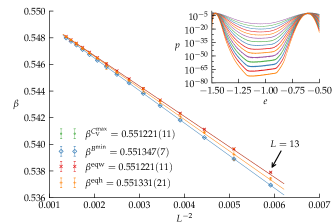
To overcome supercritical slowing down near first-order phase transitions where canonical simulations tend to get trapped in one phase and evade other problems such as hysteresis, we employed the multicanonical Monte Carlo algorithm muca . Our approach is to systematically improve guesses of the energy probability distribution using recursive estimates mucaweights before the actual production run with of the order of $(100-1000)\times 10^{6}$ sweeps for the original model and $4\times 10^{6}$ sweeps for its dual. Rare states lying between the ordered and disordered phases are then promoted artificially, decreasing the autocorrelation time and allowing the system to oscillate more rapidly between phases. For the original model (8), we took measurements only every $V=L^{3}$ sweeps to reduce the autocorrelation time $\tau_{\rm int}^{\rm meas}$ in the actual time series of the measurements. Simulations were terminated after approximately $500$ hours of real time for each lattice individually. We therefore collected less statistics for larger lattices. Still, the largest lattice of $27^{3}$ spins effectively transited more than 250 times between the two phases during the simulation, even though rare states are suppressed by more than 60 orders of magnitude compared to the most probable states (see the inset in Fig. 1). For the dual model, we took measurements every sweep, therefore the autocorrelation time $\tau_{\rm int}^{\rm meas}$ is much larger here. Canonical estimators can then be retrieved by weighting the multicanonical data to yield Boltzmann-distributed energies. Reweighting techniques are very powerful when combined with multicanonical simulations, and allow the calculation of observables over a broad range of temperatures. Errors on the measured quantities have been extracted by jackknife analysis jackknife using $20$ blocks for each lattice size.

Standard observables such as the specific heat (1) and Binder’s energy cumulant (6) have been calculated from our data as function of temperature by reweighting for both the gonihedric Ising model in Eq. (8) and its dual in Eq. (9). This enables us to determine the positions of their peaks, $\beta^{C_{V}^{\rm max}}(L)$ and $\beta^{B^{\rm min}}(L)$, with high precision. To obtain the other quantities of interest, $\beta^{\rm eqw}(L)$, and $\beta^{\rm eqh}(L)$, we use reweighting techniques to get an estimator of the energy probability densities $p(e)$ at different temperatures. $\beta^{\rm eqw}$ is chosen systematically to minimize

$$D^{\rm eqw}(\beta)=\left(\sum_{e<e_{\rm min}}p(e,\beta)-\sum_{e\geq e_{\rm min}}p(e,\beta)\right)^{2}$$ (15)

where the energy of the minimum between the two peaks, $e_{\rm min}$, is determined beforehand to distinguish between the different phases. Similarly, $\beta^{\rm eqh}$ is chosen to minimize

$$D^{\rm eqh}(\beta)=\left(\max_{e<e_{\rm min}}\{p(e,\beta)\}-\max_{e\geq e_{\rm min}}\{p(e,\beta)\}\right)^{2}$$ (16)

as function of $\beta$.

Figure 1: Best fits using the leading $1/L^{2}$ scaling obtained for the original model (8) using the (finite lattice) peak locations for the specific heat $C_{V}^{\rm max}$, Binder’s energy cumulant $B^{\rm min}$; or inverse temperatures $\beta^{\rm eqw}$ and $\beta^{\rm eqh}$, where the two peaks of the energy probability density are of same weight or have equal height, respectively. The values for $\beta^{\rm eqw}$ and $\beta^{C_{V}^{\rm max}}$ are indistinguishable in the plot. The higher order corrections which we discuss in detail in highero give the slightly different slopes. The inset shows the energy probability density $p(e)$ over $e=E/L^{d}$ at $\beta^{\rm eqh}$ for lattices with linear length $L\in\left\{13,14,\dots,26,27\right\}$.

Figure 2: Same as Fig. 1 but for the dual model (9). Here the inset shows the energy probability density $p(e)$ at $\beta^{\rm eqh}$ for lattices with linear length $L\in\left\{12,14,\dots,22,24\right\}$.

Figure 3: Plot of the goodness-of-fit parameter $Q$ for fits on the extremal locations of the specific heat, $\beta^{C_{V}^{\rm max}}$, and Binder’s energy cumulant, $\beta^{B^{\rm min}}$ of the original model for different fitting ranges $L_{\rm min}$ – $L_{\rm max}$. Upper row: Standard ($1/L^{3}$) finite-size scaling ansatz. Lower row: Transmuted ($1/L^{2}$) finite-size scaling.

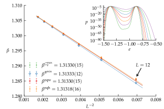
The data and fits for the inverse transition temperatures are shown in Fig. 1 for the original and in Fig. 2 for the dual model. Unusually, the estimates for $\beta^{C_{V}^{\rm max}}$ and $\beta^{\rm eqw}$ fall together because of the aforementioned equality of the ${\cal O}(L^{-4})$ corrections in the scaling ansatz for these quantities in Eqs. (Non-Standard Finite-Size Scaling at First-Order Phase Transitions) and (14). The fits have been carried out according to the non-standard scaling laws with $1/L^{2}$ corrections. We have left out the smaller lattices systematically, until a goodness-of-fit value of at least $Q=0.5$ was found for each observable individually. From error weighted averages (refraining from a full cross-correlation analysis combinefitsweigel ) of the inverse transition temperatures $\beta^{C_{V}^{\rm max}},\beta^{B^{\rm min}},\beta^{\rm eqw}$, and $\beta^{\rm eqh}$ given in Figs. 1 and 2 we find

$$\beta^{\infty} = {0.551\,291(7)},$$

$$\beta^{\infty}_{\text{dual}} = 1.313\,29(12)$$

for the infinite lattice inverse transition temperatures of the original and dual models, where the final error estimates are taken as the smallest error bar of the contributing $\beta$ estimates.

The temperature $\beta_{\text{dual}}^{\infty}$ of the dual model is related to the temperature in the original model, $\beta^{\infty}$, by the duality transformation

$$\beta^{\infty}=-\ln\left(\tanh\left(\frac{\beta_{\text{dual}}^{\infty}}{2}\right)\right)\;.$$ (17)

Applying standard error propagation, we retrieve a value of $\beta^{\infty}=0.551\,43(7)$ for the original model from dualizing $\beta^{\infty}_{\text{dual}}=1.313\,29(12)$. The estimated values of the critical temperature from the direct simulation and the simulation of the dual model are thus in good agreement, considering that higher order and exponential corrections rigorous ; fsspbc ; borgs-janke ; twophasemodel in the finite-size scaling were not included. The application of the non-standard finite-size scaling laws thus settles the enduring and very puzzling inconsistencies in previous estimates of the transition temperature for these models.

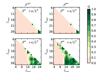
The great precision of our simulation results and the broad range of lattice sizes clearly excludes fits to the standard finite-size scaling ansatz, where the first correction is proportional to the inverse volume. This is demonstrated in Fig. 3, where the upper two plots show how the standard finite-size scaling ansatz leads to poor results. Acceptable fits are only achieved for a narrow fitting range with almost no degrees of freedom left. The fits using the non-standard laws shown in the lower plots are much better over a broad range of fitting intervals. Fits carried out using the traditional inverse volume scaling ansatz led to an inverse transition temperature of $0.549\,987(30)$ for the original model (with only $5$ degrees of freedom left per fit and $Q\approx 0.8$) and $1.310\,29(19)$ for the dual model (best fits with $2$ degrees of freedom and $Q\approx 0.3$ for all fits), which translates to $0.553\,17(11)$ using the duality relation (17). These values are about $30$ error bars apart. Since the dual model clearly displays the non-standard scaling behaviour this confirms our initial assumption that the low-temperature phase (and not just the ground state) is exponentially degenerate in this case also.

We should emphasize that the considerations described here for the gonihedric model and its dual apply generically to any models which have a low-temperature phase degeneracy which depends exponentially on the system size. Apart from higher-dimensional variants of the gonihedric model higherdG , there are numerous other fields where the scenario could be realized. Examples range from ANNNI models selke to spin ice systems gingras and topological “orbital” models in the context of quantum computing nussinov which all share an extensive ground-state degeneracy. It would be worthwhile to explore to what extent these ground states evolve as stable low-temperature phases and whether they eventually undergo a first-order transition into the disordered phase with increasing temperature. Among the orbital models for transition metal compounds, a particularly promising candidate is the three-dimensional classical compass or $t_{2g}$ orbital model compass0 where a highly degenerate ground state is well known and signatures of a first-order transition into the disordered phase have recently been found numerically compass . This has a ground-state degeneracy of $2^{3L^{2}}$ so non-standard scaling corrections, this time of $O(1/L)$, might be expected at its first-order transition point with periodic boundary conditions.

This work was supported by the Deutsch-Französische Hochschule (DFH-UFA) under Grant No. CDFA-02-07.

References

- (1) J.D. Gunton, M.S. Miguel, and P.S. Sahni, in Phase Transitions and Critial Phenomena, Vol. 8, eds. C. Domb and J.L. Lebowitz (Academic Press, New York, 1983); K. Binder, Rep. Prog. Phys. 50, 783 (1987); V. Privman (ed.), Finite-Size Scaling and Numerical Simulations of Statistical Systems (World Scientific, Singapore, 1990); H.J. Herrmann, W. Janke, and F. Karsch (eds.), Dynamics of First Order Phase Transitions (World Scientific, Singapore, 1992).
- (2) Y. Imry, Phys. Rev. B 21, 2042 (1980); K. Binder, Z. Phys. B 43, 119 (1981); M.E. Fisher and A.N. Berker, Phys. Rev. B 26, 2507 (1982).
- (3) V. Privman and M.E. Fisher, J. Stat. Phys. 33, 385 (1983); K. Binder and D.P. Landau, Phys. Rev. B 30, 1477 (1984); M.S.S. Challa, D.P. Landau, and K. Binder, Phys. Rev. B 34, 1841 (1986); P. Peczak and D.P. Landau, Phys. Rev. B 39, 11932 (1989); V. Privman and J. Rudnik, J. Stat. Phys. 60, 551 (1990).
- (4) C. Borgs and R. Kotecký, J. Stat. Phys. 61, 79 (1990); C. Borgs and R. Kotecký, Phys. Rev. Lett. 68, 1734 (1992); C. Borgs and J.Z. Imbrie, J. Stat. Phys. 69, 487 (1992).
- (5) C. Borgs, R. Kotecký, and S. Miracle-Solé, J. Stat. Phys. 62, 529 (1991).
- (6) W. Janke, Phys. Rev. B 47, 14757 (1993); W. Janke, in Computer Simulations of Surfaces and Interfaces, eds. B. Dünweg, D.P. Landau, and A.I. Milchev, NATO Science Series, II. Math., Phys. Chem. 114, 111 (2003).
- (7) C. Borgs and W. Janke, Phys. Rev. Lett. 68, 1738 (1992); W. Janke and R. Villanova, Nucl. Phys. B 489 [FS], 679 (1997).
- (8) J. Lee and J.M. Kosterlitz, Phys. Rev. B 43, 3265 (1991).
- (9) R. Pietig and F. Wegner, Nucl. Phys. B 466, 513 (1996); R. Pietig and F. Wegner, Nucl. Phys. B 525, 549 (1998).
- (10) G.K. Savvidy and F.J. Wegner, Nucl. Phys. B 413, 605 (1994); G.K. Bathas, E. Floratos, G.K. Savvidy, and K.G. Savvidy, Mod. Phys. Lett. A 10, 2695 (1995); G.K. Savvidy, K.G. Savvidy, and P.G. Savvidy, Phys. Lett. A 221, 233 (1996); D.A. Johnston and R.K.P.C. Malmini, Phys. Lett. B 378, 87 (1996).
- (11) R.V. Ambartzumian, G.S. Sukiasian, G.K. Savvidy, and K.G. Savvidy, Phys. Lett. B 275, 99 (1992); G.K. Savvidy and K.G. Savvidy, Int. J. Mod. Phys. A 8, 3393 (1993); G.K. Savvidy and K.G. Savvidy, Mod. Phys. Lett. A 8, 2963 (1993).
- (12) D. Espriu, M. Baig, D.A. Johnston, and R.K.P.C. Malmini, J. Phys. A: Math. Gen. 30, 405 (1997).
- (13) A. Lipowski, J. Phys. A: Math. Gen. 30, 7365 (1997); A. Lipowski and D. Johnston, J. Phys. A: Math. Gen. 33, 4451 (2000); A. Lipowski and D. Johnston, Phys. Rev. E 61, 6375 (2000); A. Lipowski, D. Johnston, and D. Espriu, Phys. Rev. E 62, 3404 (2000); M. Swift, H. Bokil, R. Travasso, and A. Bray, Phys. Rev. B 62, 11494 (2000); C. Castelnovo, C. Chamon, and D. Sherrington, Phys. Rev. B 81, 184303 (2010).
- (14) D.A. Johnston and R.P.K.C.M. Ranasinghe, J. Phys. A: Math. Theor. 44, 295004 (2011).
- (15) M. Mueller, W. Janke, and D.A. Johnston, Multicanonical analysis of the plaquette-only gonihedric Ising model and its dual, in preparation.
- (16) B.A. Berg and T. Neuhaus, Phys. Lett. B 267, 249 (1991); B.A. Berg and T. Neuhaus, Phys. Rev. Lett. 68, 9 (1992).
- (17) W. Janke, Physica A 254, 164 (1998).
- (18) B. Efron, The Jackknife, the Bootstrap and other Resampling Plans (Society for Industrial and Applied Mathematics, Philadelphia, 1982).
- (19) M. Weigel and W. Janke, Phys. Rev. Lett. 102, 100601 (2009); M. Weigel and W. Janke, Phys. Rev. E 81, 066701 (2010).
- (20) J. Ambjørn, G. Koutsoumbas, and G.K. Savvidy, Europhys. Lett. 46, 319 (1999); G. Koutsoumbas, G.K. Savvidy, and K.G. Savvidy, Phys. Lett. B 410, 241 (1997).
- (21) W. Selke, Phys. Rep. 170, 213 (1988).
- (22) M.J.P. Gingras, in Introduction to Frustrated Magnetism, Springer Series in Solid-State Sciences, Vol. 164, eds. C. Lacroix, P. Mendels, and F. Mila (Springer, New York, 2011), pp. 293–329.
- (23) Z. Nussinov and J. van den Brink, Compass and Kitaev models – Theory and Physical Motivations, e-print arXiv:1303.5922.
- (24) K.I. Kugel and D.I. Khomskii, Sov. Phys. Usp. 25, 231 (1982); J. van den Brink, New J. Phys. 6, 201 (2004).
- (25) S. Wenzel and A.M. Läuchli, Phys. Rev. Lett. 106, 197201 (2011); M.H. Gerlach and W. Janke, First-order directional ordering transition in the three-dimensional compass model, in preparation.