Weak gravitational lensing

Abstract

Luminous tracers have been used extensively to map the large-scale matter distribution in the Universe. Similarly the dynamics of stars or galaxies can be used to estimate masses of galaxies and clusters of galaxies. However, assumptions need to be made about the dynamical state or how well galaxies trace the underlying dark matter distribution. The gravitational tidal field affects the paths of photons, leading to observable effects. This phenomenon, gravitational lensing, has become an important tool in cosmology because it probes the mass distribution directly. In these lecture notes we introduce the main relevant quantities and terminology, but the subsequent discussion is mostly limited to weak gravitational lensing, the small coherent distortion of the shapes of distant galaxies by intervening structures. We focus on some of the issues in measuring accurate shapes and review the various applications of weak gravitational lensing, as well as some recent results.

1 Introduction

The small density fluctuations in the early Universe grow into the structures we see today under the influence of gravity. However, most of the matter responsible for structure formation remains undetectable: the visible baryonic matter makes up only $\sim 16\%$ of the total matter, the rest being dark matter. As the dark matter is believed to be collisionless and interacts only through gravity, we are fortunate that the process of structure formation can be simulated fairly well using ever larger cosmological N-body simulations. Note that this implicitly assumes that the role of baryons can be ignored, which may not always be the case, especially for future projects. The situation is reversed when we consider observations of the large-scale structure in the Universe: we are forced to rely on baryonic tracers, such as galaxies or clusters of galaxies to trace the large-scale structure. Although these are all dark matter dominated systems, their observable properties are heavily affected by highly non-linear and complex baryon physics. To match the observed abundances of galaxies and the X-ray properties of groups, AGN feedback has been suggested as an important process. Such energetic feedback affects both the mass function of halos and the matter power spectrum, thus complicating the interpretation of observations using N-body simulations as a reference.

A more direct way to relate observations to our model of structure formation would therefore be very useful. Fortunately this is possible thanks to the bending of light rays by massive structures. Such inhomogeneities in the matter distribution perturb the paths of photons that are emitted by distant galaxies. The result is equivalent to viewing these sources through a medium with a spatially varying index of refraction: the images appear slightly distorted and magnified. This phenomenon is called “gravitational lensing” because of the similarity with geometric optics. The amplitude of the distortion provides a direct measure of the gravitational tidal field, independent of the nature of the dark matter or the dynamical state of the system of interest. The lensing signal can be used to reconstruct the (projected) matter distribution, which is particularly useful for the study of clusters of galaxies, as they are dynamically young and often show signs of merging. In addition, it is possible to trace the gravitational potential out to large radii, which is typically not possible using dynamical methods.

If the deflection of the light rays is large enough, multiple images of the same source can be observed: these strong lensing events provide precise constraints on the mass on scales enclosed by these images. The discovery of a strongly lensed QSO by [1] marked the start of a new area of research, which has grown tremendously in recent years: in 1980 only 27 papers mentioned “gravitational lensing” in their abstracts, compared to 351 in 2012. Another important milestone was the discovery of strong lensing by a cluster of galaxies reported by [2], which is now seen routinely, in particular in deep observations with the Hubble Space Telescope (HST). Thanks to the large magnification provided by gravitational lensing, such deep high-resolution observations of galaxy clusters provide us with a unique view of the most distant galaxies.

The effects of gravitational lensing are not limited to small scales or to high density regions. At large radii the tidal field causes a subtle change in the shapes of galaxies, resulting in a coherent alignment of the sources that can be measured statistically. As the changes in the observed images are small, it is commonly referred to as weak gravitational lensing. The measurement of these alignments over a large area of the sky allows for the study of the statistical properties of the matter distribution which in turn can be used to constrain cosmological parameters. Other applications include the study of dark matter halos around galaxies and the study of the mass distribution in galaxy clusters. Consequently an increasing fraction of papers focuses on weak lensing: 2 of the 27 papers in 1980 contain “weak lensing” in the abstract compared to 204 out of 351 in 2012.

In these lecture notes we provide a short introduction to gravitational lensing, with the main aim to introduce the terminology. The focus of these notes will be on weak gravitational lensing and its main applications. We refer readers that wish a more thorough introduction to several excellent, comprehensive reviews. For instance, [3] introduces the theory of weak gravitational lensing as well as the key cosmological parameters and discusses the basics of shape measurements. However, the text is now over decade old, and some of the most recent insights and results are not discussed. [4] derives the expressions for gravitational lensing starting from the equation of geodesic deviation and reviews the various applications, including microlensing, which is not discussed in our notes. [5] provides an excellent recent introduction into the topic.

2 Gravitational Lensing

Light rays are deflected when they travel through an inhomogeneous medium (following Fermat’s principle). In geometric optics the quantity that determines the change in the photon’s path is the index of refraction. In the case of gravitational lensing the situation is very much the same, except that the gravitational potential replaces the role of the index of refraction. In a cosmological setting we make several additional assumptions. First of all, we will assume that the gravitational field is weak (i.e. we are not considering the bending of light rays around black holes or close to neutron stars) and that the angles by which light rays are deflected are small. Finally, we consider the “thin lens” approximation: the deflection occurs on scales that are much smaller than the size of the Universe, i.e., the thickness of the lens is much smaller than the distance between the observer, lens, and source. This is a very reasonable assumption as galaxy clusters (the most massive objects that we study) extend at most a few Megaparsec, whereas the sources are Gigaparsecs away. We also assume the lens is static, because the light crossing time is short compared to the dynamical time scale.

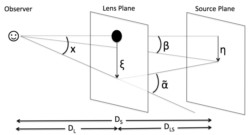
Figure 1: Geometry of the lensing problem

2.1 Lens Equation

Figure 1 shows a schematic of the deflection of a light ray that passes a deflector at a distance ${\mathbf{\xi}}$ in the lens plane. If we project the location of the lens onto the source plane, the source is separated by a distance ${\mathbf{\eta}}$. From the Figure it is easy to see that the two positions are related through

$${\mathbf{\eta}}=\frac{D_{S}}{D_{L}}{\mathbf{\xi}}-D_{LS}{\mathbf{\tilde{\alpha}}}({\mathbf{\xi}}),$$ (1)

where $D_{S}$, $D_{L}$ and $D_{LS}$ are the angular diameter distances between the observer and source, the observer and the lens, and the lens and the source, respectively. As we observe objects projected on the sky, it is more convenient to define angular coordinates such that ${\mathbf{\eta}}=D_{S}{\mathbf{\beta}}$ and ${\mathbf{\xi}}=D_{L}{\mathbf{x}}$: a source with a true position ${\mathbf{\beta}}$ will be observed at a position ${\mathbf{x}}$ on the sky. In fact, images of the source will appear at all locations ${\mathbf{x}}$ that satisfy the lens equation

$${\mathbf{\beta}}={\mathbf{x}}-\frac{D_{LS}}{D_{S}}{\mathbf{\tilde{\alpha}}}(D_{L}{\mathbf{x}})\equiv{\mathbf{x}}-{\mathbf{\alpha}}({\mathbf{x}}),$$ (2)

where we defined the scaled deflection angle ${\mathbf{\alpha}}({\mathbf{x}})$. Although the lens equation is thus expressed rather conveniently, the physical interpretation still requires estimates for the lens and source redshifts. In the case of strong gravitational lensing one can perhaps afford to obtain these through deep spectroscopy, but in the case of weak gravitational lensing, where the shapes of large numbers of galaxies are measured, we rely on photometric redshift estimates instead. Although obtaining these is a critical part for a correct interpretation of the lensing signal, in these lectures we will discuss this issue only briefly in §6.1.

2.2 Delay

As can be seen from Figure 1 the total path length, and thus the amount of time the deflected photon travels, is modified. If we imagine a source that produces a burst of light, the photons will arrive at a time

$$\tau=\frac{1+z_{L}}{H_{0}}\frac{D_{L}D_{S}}{D_{LS}}\left[\frac{1}{2}({\mathbf{x}}-{\mathbf{\beta}})^{2}-\Psi_{2D}({\mathbf{x}})\right],$$ (3)

where the first term quantifies the increase in the path length and the second term the “slowing down” as the photon travels through the gravitational potential $\Psi_{2D}$. The latter is related to the projected mass distribution through

$$\Psi_{2D}({\bf x})=\frac{1}{\pi}\int{\rm d}^{2}{\bf x^{\prime}}\kappa({\bf x^{\prime}})\ln|{\bf x-x^{\prime}}|,$$ (4)

where the convergence $\kappa$ is the ratio of the projected surface density $\Sigma({\bf x})$ and the critical surface density $\Sigma_{\rm crit}$:

$$\kappa({\bf x})=\frac{\Sigma({\bf x})}{\Sigma_{\rm crit}},$$ (5)

with $\Sigma_{\rm crit}$ defined as

$$\Sigma_{\rm crit}=\frac{c^{2}}{4\pi G}\frac{D_{S}}{D_{L}D_{LS}}.$$ (6)

Note that, analogous to the Poisson equation, $\kappa=\frac{1}{2}\nabla^{2}\Psi_{2D}$.

Following Fermat’s principle, images are formed at the extrema of the light arrival surface, i.e., where $\nabla{\mathbf{\tau}}=0$; the result is once more the lens equation, while demonstrating that ${\mathbf{\alpha}}=\nabla\Psi_{2D}$. As the actual arrival times will typically differ between images, variations in the source brightness will also appear at different times. Provided one has an accurate model for the deflection potential and has measured the time delays (as well as the redshifts for the lens and source), the remaining key parameter in Eqn. 3 is the Hubble parameter $H_{0}$. Hence time delays provide an interesting, independent approach to measure the Hubble parameter [6, 7]. The main limitation of this method is the uncertainty in the mass distribution. Recent studies (e.g., [8]) have taken care to model the contributions from additional deflectors, but [9] pointed out that degeneracies in the mass model may ultimately limit the accuracy.

2.3 Deflection

In most applications of gravitational lensing the actual deflection is not observed, because the true position of the source is unknown. As a consequence only the effects of differential deflection (=distortion) can be measured. Furthermore the surface brightness is preserved. However, CMB photons are also deflected and as a result the observed temperature $\tilde{T}({\bf x})$ is in fact (see e.g., [10], for a review):

$$\tilde{T}({\bf x})=T({\bf x}+\nabla\Psi)\approx T({\bf x})+\nabla\Psi\cdot\nabla T({\bf x}).$$ (7)

Hence gravitational lensing changes the statistical properties of the temperature fluctuations, resulting in a smoothing of the acoustic peaks in the power spectrum (e.g., [11, 10]). Furthermore, the measurement of the 4-point function can be used to measure the lensing signal directly and map the mass distribution, albeit on very large scales (e.g.,[12]). This signal has been recently detected at in ground-based experiments ([13, 14]) and by Planck from space ([15]).

2.4 Differential Deflection

Analogous to the case of the CMB sky the observed surface brightness of a distant galaxy is remapped. If the deflection angle and its spatial variation are small (compared to the extent of the source), this mapping can be linearized:

$$f^{\rm obs}({\bf x})=f^{\rm s}[{\mathbf{\beta}}({\bf x})]\approx f^{\rm s}({\cal A}{\bf x}),$$ (8)

with $f^{\rm s}({\bf x})$ the unlensed surface brightness and $\cal A$ the Jacobian of the transformation. This regime is commonly referred to as “weak gravitational lensing”. The distortion matrix can be written in terms of derivatives of the deflection angle, and thus in terms of second derivatives of the deflection potential:

$${\cal A}=\delta_{ij}-\frac{\partial^{2}\Psi}{{\partial x_{i}\partial x_{j}}}=\left(\begin{array}[]{cc}1-\kappa-\gamma_{1}&-\gamma_{2}\\ -\gamma_{2}&1-\kappa+\gamma_{1}\\ \end{array}\right)=(1-\kappa)\left(\begin{array}[]{cc}1-g_{1}&-g_{2}\\ -g_{2}&1+g_{1}\\ \end{array}\right),$$ (9)

where we introduced the complex shear ${\bf\gamma}\equiv\gamma_{1}+i\gamma_{2}$, and defined the reduced shear $g_{i}=\gamma_{i}/(1-\kappa)$. The shear is related to the deflection potential through

$$\gamma_{1}=\frac{1}{2}\left(\frac{\partial^{2}\Psi}{\partial x_{1}^{2}}-\frac{\partial^{2}\Psi}{\partial x_{2}^{2}}\right)\hskip 10.00002pt{\rm and}\hskip 10.00002pt\gamma_{2}=\frac{\partial^{2}\Psi}{\partial x_{1}\partial x_{2}},$$ (10)

The effect of the remapping by ${\cal A}$ is to transform a circular source into an ellipse with axis ratio $\sim(1-|g|)/(1+|g|)$ and position angle $\alpha=0.5\arctan(g_{2}/g_{1})$; the reduced shear describes the anisotropic distortion of a source. If $\kappa\ll 1$ (i.e., the weak lensing regime), the observable $g_{i}\sim\gamma_{i}$. In addition, the source is magnified by a factor

$$\mu=\frac{1}{\det\cal{A}}=\frac{1}{(1-\kappa)^{2}-|\gamma|^{2}}=\frac{1}{(1-\kappa)^{2}(1-|g|^{2})},$$ (11)

boosting the observed flux by the same amount. To first order, the magnification depends on the convergence only; i.e. $\kappa$ describes the isotropic distortion of a source (contraction or dilation). Both the shearing and magnification of sources are observable effects, although both are quite different in terms of techniques and systematics. The measurements are, however, statistical in nature, because the signal cannot be inferred from individual sources.

The measurement of the shear involves measuring the shapes of galaxies and we will discuss some of the practical issues below. The effect of weak gravitational lensing is to change the unlensed ellipticity of a galaxy, $\epsilon_{\rm orig}=(a-b)/(a+b)$, where $a$ is the semi-major axis, and $b$ the semi-minor axis, to an observed value:

$$\epsilon^{\rm obs}=\frac{\epsilon^{\rm orig}+g}{1+g^{*}\epsilon^{\rm orig}}\approx\epsilon^{\rm orig}+\gamma,$$ (12)

where the asterisk denotes the complex conjugate. Only if the shear is larger than $\epsilon^{\rm orig}$ does the observed ellipticity of a single galaxy provide a useful estimate of the shear. A population of intrinsically round sources would therefore be ideal, but unfortunately real galaxies have an average intrinsic ellipticity of $\sim 0.25$ per component (e.g., [16]). Instead the lensing signal is inferred by averaging over an ensemble of sources, under the assumption that the unlensed orientations are random. Although this assumption has been adequate up to now, the increased precision of future weak lensing studies requires that the contribution from intrinsic alignments is taken into account.

Intrinsic alignments are expected to arise because of tidal torques, or alignments of the angular momentum, when galaxies form during the collapse of a filament. For instance it has been known for a while that the central galaxies in clusters point towards each other ([17]). In general one expects the orientation of central galaxies to be correlated with the large scale mass distribution they formed in. Early numerical simulations also show strong alignments between halos (e.g., [18, 19]), albeit with amplitudes that are already ruled out by observations. This highlights the difficulty in predicting the alignment signal, because the outer regions of a halo are more easily aligned than the inner, baryon-dominated regions, which are what we actually observe. For instance initial alignments between the angular momentum of baryons and the halo can be erased through the violent process of galaxy formation. Hence, the study of intrinsic alignments, although a source of bias for cosmic shear studies, provides a unique probe of baryon physics. Although further progress is expected from hydrodynamic numerical simulations, direct observational constraints are needed. This requires precise redshift information for the galaxies in question. Fortunately high-quality photometric redshifts can also be used to this end.

The intrinsic alignment signal has been detected for early type galaxies (e.g., [20, 21, 22, 23]). The alignment of late type galaxies is believed to arise from alignments in the angular momentum, and has proven more difficult to constrain observationally. Finally the local torques may align satellite galaxies within a halo such that they preferentially point towards the host ([24]). Some tentative detections of such radial alignment have been reported (see [25] for a discussion of results), but significant progress is expected in the coming years thanks to the combination of large imaging surveys with adequate spectroscopic observations.

The intrinsic alignments between galaxies that are physically associated can be readily reduced by avoiding correlating the shapes of galaxies at similar redshifts and using cross-correlations between galaxies with different redshifts instead. However, an additional consequence of intrinsic alignments was found by [26]. It arises because galaxy shapes may be correlated with the surrounding density field (e.g. the radial alignments of satellite galaxies mentioned above). As this density field is also the source of the lensing signal the combination of a radial alignment at the lens redshift and a tangential alignment of the sources, leads to a suppression of the lensing signal. As this leads to anti-correlations between shapes of galaxies at different redshifts it cannot be easily corrected for. The signal can be suppressed, but only with a great loss in precision. Therefore the current approach is to model the intrinsic alignment as part of the cosmological analysis (e.g., [27, 28]).

As is the case for the shear, we cannot measure the actual magnification of a single object because the intrinsic flux and size are typically unknown. Instead, the signal can be inferred from the change in the source number counts, which is determined by the balance between two competing effects. On the one hand the actual volume that is surveyed is reduced, because the solid angle behind the cluster is enlarged. On the other hand the fluxes of the sources in this smaller volume are boosted, thus increasing the limiting magnitude. As a consequence, the net change in source surface density depends not only on the mass of the lens, but also on the steepness of the intrinsic luminosity function of the sources. If it is steep, the increase in limiting magnitude wins over the reduction in solid angle, and an excess of sources is observed. If the number counts instead are shallow, a reduction in the source number density is observed.

One interesting recent application of magnification is the study of the lensing signal around high-redshift lenses using Lyman break galaxies (LBGs) as sources at $z>3$. Although these galaxies are too faint and too small to have their shapes determined accurately, their magnitudes can still be measured. The feasibility of this approach was demonstrated by [29] who studied the signal around lenses at intermediate redshifts. Magnification studies are particularly interesting to study high redshift lenses, because the number density of sources for which shapes can be measured decreases with redshift (especially for ground-based data). For instance, [30] measured the mass of $z\sim 1$ clusters of galaxies and recently [31] were able to constrain the masses of a sample of distant submillimetre galaxies.

2.5 Mass reconstructions

The shear and convergence can both be derived from the second derivatives of the deflection potential. If we consider the definition of $\Psi_{2D}$ given by Eqn. 4 and compute the shear following Eqn. 10 we find that the shear can be written as a convolution of the convergence with a kernel $\chi({\bf x})$:

$$\gamma({\bf x})=\frac{1}{\pi}\int{\mathrm{d}}^{2}{\bf x^{\prime}}\chi({\bf x-x^{\prime}})\kappa({\bf x^{\prime}}),$$ (13)

where the convolution kernel $\chi({\bf x})$ is given by

$$\chi({\bf x})=\frac{x_{2}^{2}-x_{1}^{2}-2ix_{1}x_{2}}{|{\bf x}|^{4}}.$$ (14)

It is also possible to express the surface density in terms of the observable shear by inverting this expression (as was first shown by [32]). The resulting ”mass reconstruction” $\hat{\kappa}$ is given by

$$\hat{\kappa}({\bf x})-\kappa_{0}=\frac{1}{\pi}\int{\mathrm{d}}^{2}{\bf x^{\prime}}\chi^{*}({\bf x-x^{\prime}})\gamma({\bf x^{\prime}}),$$ (15)

where the constant $\kappa_{0}$ shows that the surface density can only be recovered up to a constant. This reflects the fact that a constant $\kappa$ does not cause a shear. In fact one can show that a transformation $\kappa^{\prime}=\lambda\kappa+(1-\lambda)$ leaves the reduced shear unchanged. This complication is known as the mass-sheet degeneracy ([33]). Note that $\kappa({\bf x})$ is a real function, which may not be the case for the actual mass reconstruction. A non-negligible imaginary component of $\hat{\kappa}$ is a sign of systematics in the data and thus can be used to identify problems with the data analysis.

The possibility to reconstruct the surface mass density is clearly an important application of weak gravitational lensing: it allows us to directly map the total mass distribution, which is particularly interesting in the case of merging clusters of galaxies. Note, however, that Eqn. 15 cannot be used in practice as evaluating it requires data out to infinity. Additional complications are the fact that shear is only sampled at the locations of the sources and the fact that we observe the reduced shear rather than the shear itself. Several solutions have been proposed, such as finite field inversions (e.g., [34, 35]) or maximum likelihood methods (e.g., [36, 37]). A question that has renewed interest in this area is whether the statistics of the mass reconstruction can be used for cosmological parameter estimation. For instance [38] detected the second-, third- and fourth-order moment of the distribution of the convergencem map. Although comparison with simulations suggested fair agreement, more work is needed to understand the biases that might arise.

Figure 2 shows an example of the usefulness of a mass reconstruction: the central regions of the $z=0.83$ cluster MS1054-03 show significant substructure based on a weak lensing analysis of deep HST observations by [39]. It is clear that the mass distribution cannot be described by a simple model, nor can one assume that the cluster is dynamically relaxed.

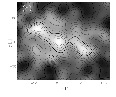
Figure 2: Left panel: mass reconstruction of the central region of the $z=0.83$ cluster of galaxies MS1054-03 from [39] demonstrating that the complex mass distribution is not well described by a simple parametric model. Right panel: the azimuthally averaged tangential distortion as a function of distance to the cluster center. The drop in signal at $r~{}20-50^{\prime\prime}$ before rising again is the result of the complex mass distribution seen in the mass reconstruction.

One of the best-known weak lensing results is the mass reconstruction of the “Bullet cluster” 1ES 0657-558 by [40]. This is an advanced stage of a merger of two clusters of galaxies, in which the lower mass cluster has already passed through the core of the main body. The mass reconstruction, based on deep HST data, shows a significant separation of the baryons (in the form of the hot X-ray emitting gas) and the dark matter, as inferred from weak lensing. Due to its collisional nature the gas has been slowed down in the collision, whereas the dark matter halos have passed through each other without significant interaction. What makes this a particularly important observation is that the significant displacement between the baryonic mass and the peaks in the lensing map cannot be (easily) explained without dark matter.

2.6 Mass estimates

As the calculation of the mass reconstruction involves smoothing the data, the results are not ideal if one wants to measure masses. Instead one can fit a parameterized model to the observed shear field, but as we saw, this may not be accurate in the case of merging systems. It is, however, possible to obtain an estimate of the projected mass within an aperture, with relatively few assumptions about the actual mass distribution. It makes use of the fact that for any mass distribution the azimuthally averaged tangential shear $\langle\gamma_{T}\rangle$ as a function of radius from the cluster center measures a contrast in surface density

$$\langle\gamma_{T}\rangle(r)=\frac{\bar{\Sigma}(<r)-\bar{\Sigma}(r)}{\Sigma_{\rm crit}}=\bar{\kappa}(<r)-\bar{\kappa}(r),$$ (16)

where the tangential shear is defined as

$$\gamma_{T}=-(\gamma_{1}\cos 2\phi+\gamma_{2}\sin 2\phi),$$ (17)

where $\phi$ is the azimuthal angle with respect to the lens. For this reason the tangential shear is a very convenient way to represent the lensing signal around a single massive lens (e.g. a galaxy cluster) or a sample of lenses (galaxies or groups). In addition to the tangential shear, one can also define a cross shear $\gamma_{\times}$, which is equivalent to rotating sources by 45 degrees and measuring the corresponding tangential shear. The azimuthally averaged $\gamma_{\times}$ should vanish in the absence of systematics (similar to the imaginary part of the mass reconstruction discussed earlier).

Due to the substructure in the central regions of MS1054-03, the resulting tangential shear, shown in the right panel of Figure 2, does not decline monotonically. Hence the tangential shear profile cannot always be interpreted by fitting simple parameterized models, such as an isothermal sphere or NFW profile, to the data. Similarly at large radii the lensing signal around a sample of galaxies is sensitive to their clustering properties. A correct interpretation thus becomes more involved, although the halo-model has been quite successful in this regard (see §LABEL:sec:halo_model). In the case of galaxy clusters one can use aperture mass statistics, such as the $\zeta_{c}$ estimator proposed by [41]

$$\zeta_{c}(r_{1})=2\int_{r_{1}}^{r_{2}}d\ln r\langle\gamma_{t}\rangle+\frac{2r_{\rm max}^{2}}{r_{\rm max}^{2}-r_{2}^{2}}\int_{r_{2}}^{r_{\rm max}}d\ln r\langle\gamma_{t}\rangle,$$ (18)

which can be expressed in terms of the mean dimensionless surface density interior to $r_{1}$ relative to the mean surface density in an annulus from $r_{2}$ to $r_{\rm max}$:

$$\zeta_{c}(r_{1})=\bar{\kappa}(r^{\prime}<r_{1})-\bar{\kappa}(r_{2}<r^{\prime}<r_{\rm max}).$$ (19)

Although the surface density in the outer annulus should be small for results based on wide field imaging data, it cannot be completely ignored. Its value can be estimated using parametric models resulting in a rather weak model dependence of the projected mass estimate. The resulting estimate for the projected mass in the aperture is thus rather robust, but comparison to other (baryonic) proxies for the mass is typically not as straightforward, as this does require assumptions about the geometry of the cluster.

3 Measuring galaxy shapes

The typical change in ellipticity due to gravitational lensing is much smaller than the intrinsic shape of the source, even in the case of clusters of galaxies. Although this can be dealt with by averaging the shapes of many galaxies, the shear signal can be overwhelmed by instrumental effects, which may be difficult to assess on an object-by-object basis. Hence the study of algorithms that can accurately determine the shapes of faint galaxies has been a major part of the development of weak gravitational lensing as a key tool for cosmology.

The problem is highlighted by comparing the ”true” image of an object to the ”observed” version shown in Figure 3. The main source of bias that needs to be corrected for is the blurring of the images by the point spread function (PSF). Unless the pixels are large with respect to the PSF, the pixellation is not a major source of concern. As it is easier to measure properties when the noise is low, the S/N ratio is another key parameter determining how well shapes can be measured. In the case of space-based observations, due to the combination of low sky background and radiation damage, charge transfer inefficiency may also be an important effect (e.g., [42]).

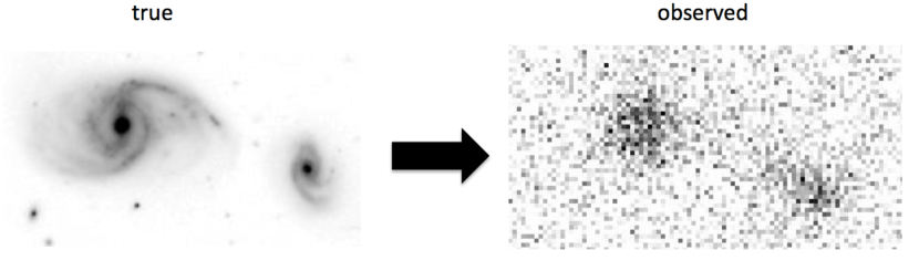
Figure 3: We need to infer accurate information about the shape of the true surface brightness distribution (left) from images that have been corrupted by various sources of bias, such as pixellation, seeing and noise. Given a good description of the instrumental effects it is possible to simulate their effects and thus examine the performance of shape measurement algorithms.

One approach to recover the true galaxy shapes is to adopt a suitable model of the surface brightness distribution. An estimate of the lensing signal is obtained by shearing the model and convolving it with the PSF, comparing the result to the observed image until a best fit is found. A model for the PSF is typically obtained by analyzing the shapes of a sample of stars in the actual data. An important advantage of this approach is that instrumental effects can be incorporated in a Bayesian framework. As the modeling requires many calculations and thus is computationally expensive, the use of model-fitting algorithms has only recently become more prominent. Some examples of this approach are lensfit ([43]) which was used to analyze the CFHTLenS data, and im3shape ([44]). There are challenges as well: the model needs to accurately describe the surface brightness of the galaxies, while having a limited number of parameters in order to avoid fitting the noise. A model that is too rigid will lead to model bias (e.g., [45]), as does a model that is too flexible.

Galaxy shapes can also be quantified by computing the moments of the galaxy images. Such methods have been applied to data extensively, especially the method proposed by [46]. The shapes can be quantified by the polarization

$$e_{1}=\frac{I_{11}-I_{22}}{I_{11}+I_{22}},~{}{\rm and}~{}e_{2}=\frac{2I_{12}}{I_{11}+I_{22}},$$ (20)

where the quadrupole moments $I_{ij}$ are given by

$$I_{ij}=\frac{1}{I_{0}}\int{\rm d}^{2}{\mathbf{x}}~{}x_{i}x_{j}W({\mathbf{x}})f({\mathbf{x}}),$$ (21)

where $f({\mathbf{x}})$ is the observed galaxy image, $W({\mathbf{x}})$ a suitable weight function to suppress the noise and $I_{0}$ the weighted monopole moment. It is also convenient to define $R^{2}=I_{11}+I_{22}$ as a measure of the size of the galaxy. Both model-fitting and moment-based methods are used to measure the weak lensing signal and further development is ongoing. In these notes we continue with a closer look at the use of moments, because it is somewhat easier to see how the results are impacted by instrumental effects.

3.1 Observational distortions

The observed moments are changed by the blurring of the PSF: the PSF has a width which leads to rounder images and typically is anisotropic, which leads to a preferred orientation. If that were not enough, noise in the images leads to additional biases. The various sources of bias can be grouped into two kinds: a multiplicative bias $m$ that scales the shear, and an additive bias $c$ that reflects preferred orientations that are introduced. The observed shear and true shear are thus related by (e.g., [47]):

$$\gamma_{i}^{\rm obs}=(1+m)\gamma_{i}^{\rm true}+c,$$ (22)

where we implicitly assumed that the biases are the same for both shear components. The additive bias is a major source of error for cosmic shear studies because the PSF patterns can overwhelm the lensing signal. Studies of clusters and galaxies use the tangential shear averaged using many lens-source pairs, and much of the additive biases tend to average away. As we discuss below it is possible to test how well the correction for additive bias has performed, but the estimate of the multiplicative bias requires image simulations.

If it were possible to ignore the effects of noise in the images, we could use unweighted moments. In this case the correction for the PSF is straightforward as the corrected moments are given by

$$I^{\rm true}_{ij}=I^{\rm obs}_{ij}-I^{\rm PSF}_{ij},$$ (23)

i.e. one only needs to subtract the moments of the PSF from the observed moments. The result provides an unbiased estimate of the polarization, but to convert the result into a shear still requires knowledge of the unlensed ellipticity (distribution), although this could be established iteratively from the data.

From a pure statistical perspective it is more efficient to image large areas of the sky rather than take deep images of smaller regions (e.g., [48]). Hence the images of the sources are typically noisy and unweighted moments cannot be used. The optimal estimate is obtained by matching the weight function to the size (and shape) of the galaxy image. However, the correction for the change in moments due to both the weight function and the PSF is no longer simple, but involves higher order moments of the surface brightness distribution, which themselves are affected by noise (e.g., [42, 49]). Note that limiting the expansion in moments is analogous to the model bias in model-fitting approaches.

[42] present a detailed breakdown of the various sources of bias that affect weak lensing analyses and interested readers are encouraged to examine the findings of that paper. For instance, in the simplified case of unweighted moments, the change in the observed ellipticity $\hat{\epsilon}$ due to small errors in the PSF size $(\delta R^{2}_{\rm PSF})$ or PSF ellipticity $(\delta\epsilon_{\rm PSF})$ can be expressed as

$$\hat{\epsilon}_{\rm gal}\approx\epsilon_{\rm gal}+\frac{\partial\epsilon_{\rm gal}}{\partial(R^{2}_{\rm PSF})}\delta(R^{2}_{\rm PSF})+\frac{\partial\epsilon_{\rm gal}}{\partial\epsilon_{\rm PSF}}\delta\epsilon_{\rm PSF},$$ (24)

which can be written as

$$\hat{\epsilon}_{\rm gal}\approx\left[1+\frac{\delta(R^{2}_{\rm PSF})}{R^{2}_{\rm gal}}\right]\epsilon_{\rm gal}-\left[{\frac{R^{2}_{\rm PSF}}{R^{2}_{\rm gal}}\delta\epsilon_{\rm PSF}+\frac{\delta(R^{2}_{\rm PSF})}{R^{2}_{\rm gal}}\epsilon_{\rm PSF}}\right].$$ (25)

The first term shows the multiplicative bias caused by errors in the PSF size, relative to the galaxy size. The second term corresponds to the additive bias and is determined by errors in the PSF model $\delta\epsilon_{\rm PSF}$ and residuals in the correction for the PSF anisotropy (last term). However, the PSF is not the only source of bias, especially when considering weighted moments and hence the expression for the multiplicative bias (idem for the additive one) becomes more involved when more effects are included (see [42] for details). In particular new contributions arise that are related to the correction method (method bias). As is already clear from the expression reproduced above, a small PSF is important in order to minimize the biases. Although small PSF anisotropy is preferable, a good model of the PSF size and shape is critical.

Figure 4: Left panel: Plot of the apparent magnitude versus half-light radius for RCS data from [50]. The rectangle indicates the sample of stars that can be used to model the PSF variation. Brighter stars saturate and their observed sizes increase as can be seen as well. Right panel: An example of the pattern of PSF anisotropy for MegaCam on CFHT from [51]. The sticks indicate the direction of the major axis of the PSF and the length is proportional to the PSF ellipticity. A coherent pattern across the field-of-view is clearly visible.

3.2 PSF model

Although much effort has been spent on improving the correction for the PSF, without an accurate model for the spatial variation of the PSF, the resulting signal will nonetheless be biased (e.g., [52]). In ground-based data the PSF changes from exposure to exposure due to changing atmospheric conditions and gravitational loads on the telescope. The PSF of HST observations changes due to the change in thermal conditions as it orbits around the Earth. If a sufficient number of stars can be identified in the images, these can be used to model the PSF. As can be seen from Figure 4 stars can be identified by plotting magnitude versus size. As the stars are the smallest objects, they occupy a clear vertical locus. If the star saturates, charge leaks into neighboring pixels and the size increase which explains the trail towards larger sizes, whereas the size and shape estimates become noisy for faint stars. After selecting a sample of suitable stars (not too bright such that they are saturated but also not too faint such that they cannot be separated from faint, small sources) the resulting PSF pattern can be modeled. The right panel in Figure 4 shows an example for MegaCam on the Canada-France-Hawaii Telescope (CFHT), which shows a coherent pattern across the field-of-view.

Most studies to date fit an empirical model to the measurements of a sample of stars to capture the spatial variation. As the PSF pattern is determined by (inevitable) misalignments in the optics, the overall pattern varies relatively smoothly. However, to efficiently image large areas of sky, observations are carried out using mosaic cameras. For instance, Megacam on CFHT consists of 36 chips. Misalignments and flexing of the chips will lead to small additional PSF patterns on the scale of the chips. A single low-order model fit to the full focal plane cannot capture these small scale variations. Instead a low-order (typically second-order) polynomial is used for each chip, but this may lead to over-fitting on small scales due to the limited number of stars per chip. [53] examined whether a model based on the typical optical distortions can be used to model the PSF pattern of the Subaru telescope (also see [54]). The global pattern, which varies from exposure to exposure, can indeed be described fairly well. By combining many observations, one can also try to account for the misalignments of the individual chips.

To obtain deeper images and to fill in the gaps between the chips, exposures are dithered and combined into a stack. As the observing conditions typically vary between exposures, the combined PSF pattern becomes very complicated (especially at the location of the chip gaps). It is important to account for this, for instance by modeling the PSF of each exposure and keeping track which PSFs contribute to the stack at a particular location [55]. Alternatively one can model each exposure, which is the approach used in [43].

The true shapes of galaxies should not correlate with the PSF pattern, although chance alignments of the shear and the PSF may occur. This enables an important test of the fidelity of the correction for PSF anisotropy: we can measure the correlation between the corrected galaxy shapes and the PSF ellipticity, the star-galaxy correlation. The detection of a significant correlation points to an inadequate correction, which may be due to the method itself or the PSF model. A detailed discussion and application of this test is presented in [56]. Importantly, this test does not depend on cosmology, while being very sensitive to one of the most dominant sources of bias in cosmic shear studies. In the analysis of the CFHTLenS data, presented in [56] this was used to identify and omit fields that showed significant systematics.

3.3 Image Simulations

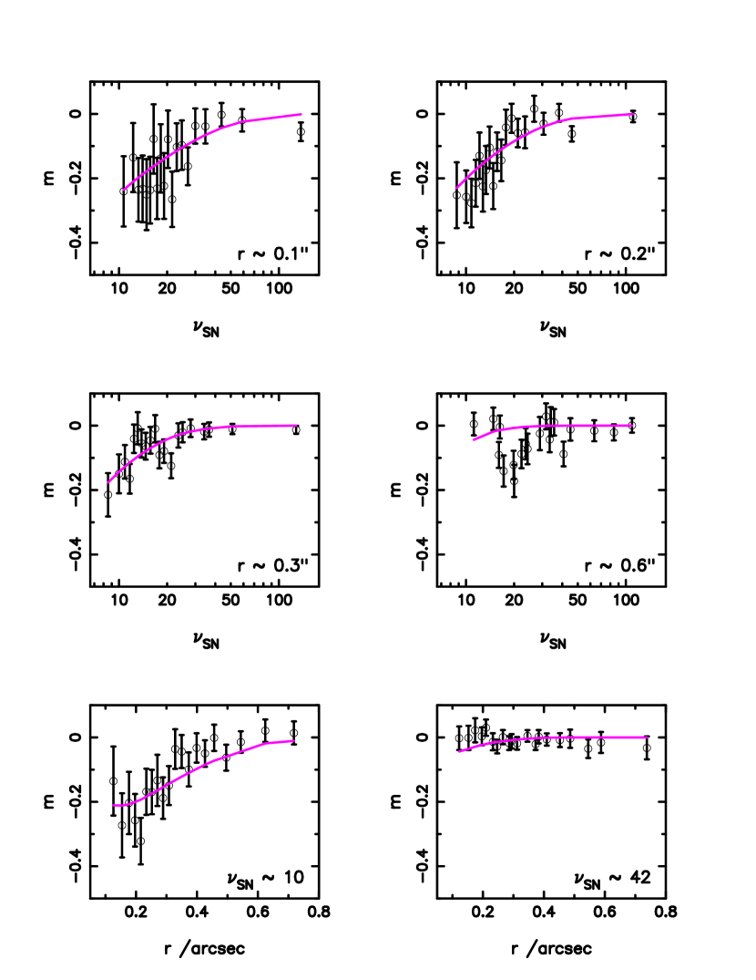
Figure 5: Multiplicative bias $m$ as a function of signal-to-noise ratio $\nu_{\rm SN}$ for galaxies with different sizes measured by lensfit from [43]. The solid curves are the result of a fitting function matched to a wide range in size and S/N.

The star-galaxy correlation function is a sensitive test of the correction for additive bias, but no such test exists for the multiplicative bias. Instead the performance of an algorithm needs to be determined by applying it to simulated data where the input shear is known. As an example Figure 5 shows the recovered multiplicative bias $m$ for lensfit from [43]. The bias increases as the signal-to-noise ratio $\nu_{\rm SN}$ decreases. The bias also depends on the size of the of the sources, with a larger bias for smaller objects. These results can be used to find an empirical correction as a function of the object properties, thus reducing the bias to an acceptable level.

Several community-wide blind studies have been carried out to provide a bench-mark for the performance of weak lensing studies. The first of these was the Shear TEsting Programme (STEP;[47]), which simulated observations using simple models for the galaxies. This was followed by STEP2 ([57]) using synthetic galaxies based on HST data. These results showed a range in multiplicative biases, with some methods finding biases as small as $\sim 1\%$. These initiatives were followed by GREAT08 ([58]) and GREAT10 ([59]) which were more systematic investigations of the sources of bias.

As the bias depends on the galaxy properties, in particular the S/N and size, it is important that image simulations match the observations. If this is not the case, the resulting bias may not be representative for the actual data. For instance the lack of faint galaxies in STEP1 leads to an underestimate of the bias compared to that of actual data. For instance new studies find that one needs to include galaxies at least 1.5 magnitudes fainter than the limiting magnitude of the source sample. As mentioned earlier, the bias in shape measurement algorithms also depends on the intrinsic ellipticity distribution (also see [60]). Hence, in order to examine the performance of the algorithms, the fidelity of the simulations themselves is critical. With the more stringent requirements of future experiments, this is an important area of development.

4 Lensing by Clusters

The first attempt to detect a weak lensing signal was made by [61] who stacked a sample of galaxies, with shapes measured from photographic plates. However, it was the advent of CCD cameras with their improved performance and the possibility to correct for systematics that allowed for the first detections of the lensing signal. As the amplitude of the lensing signal is proportional to the mass of the lens, galaxy clusters provided a natural target for these pioneering studies. The first detection of the lensing signal, around the massive cluster Abell 1689, was presented by [62]. The cluster studies carried out in the ’90s demonstrated the feasibility of weak lensing and thus paved the way for the other applications of weak lensing, in particular the cosmic shear.

Cluster samples are increasing rapidly thanks to large surveys at various wavelengths that aim to use the evolution in the number density of clusters to constrain cosmological parameters. To do so, however, requires the calibration of the scaling relations between the observed properties and the cluster masses. As numerical simulations cannot (yet) capture the full effects of the complex baryon physics, and dynamical methods are biased, weak lensing masses provide important information. Another application, which we already encountered when we discussed the usefulness of mass reconstructions, is the study of merging clusters. A recent review of lensing studies of galaxy clusters can be found in [63].

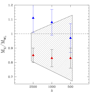
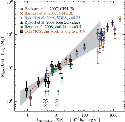
Figure 6: Left panel: the ratio of the hydrostatic mass, derived from X-ray observations, to the weak lensing mass as a function of density contrast for cool-core clusters (blue triangles) and non-cool-core systems (red triangles) reproduced from [64]. The shaded region shows the predictions from numerical simulations. Right panel: from [65] showing the scaling relation between lensing mass and X-ray luminosity for stacked galaxy groups in the COSMOS field and literature results for massive clusters.

Several studies have recently released results for samples of $\sim 50$ well-known massive clusters ([66, 67, 68, 69]). Such large samples allow us to compare scaling relations and examine their intrinsic scatter. These results may help to identify shortcomings of numerical simulations. For instance [70] found that $Y_{X}=M_{\rm gas}T_{X}$, i.e. the product of gas mass and X-ray temperature, showed the smallest scatter in their hydrodynamic simulations. [64], however, found that the gas mass itself has the smallest intrinsic scatter, although they note that the scatter in $Y_{X}$ is the same for different subsamples of clusters, which may be a useful property for cluster surveys. Numerical simulations have long suggested that hydrostatic cluster masses are biased low because of turbulent motions in the gas. Weak lensing studies have now confirmed this, and an example is presented in the left panel of Figure 6, showing the results from [64].

Individual masses can only be determined for the most massive clusters of galaxies, thus significantly limiting the mass range that can be studied. However, the lensing signal is directly proportional to the mass, which allows us to stack the signals of lower mass systems if we sort these by baryonic properties. This is useful, because the scaling relations for low mass systems are affected more by feedback processes. The right panel of Figure 6 shows the results of an analysis of the stacked weak lensing signal around groups discovered in the COSMOS field. [65] presented a comparison of the lensing mass and the X-ray luminosity. Complementing the results with literature results from massive clusters, the results suggest that a single power-law relation can describe the observations. Stacking also allows one to trade depth against survey area, with the SDSS results presented by [71] being a nice example; although the SDSS data are too shallow to detect a significant signal for individual clusters, the large number of targets allowed for precise measurements over a wide range in cluster richness.

5 Lensing by Galaxies

Although the large dynamical mass for the Coma cluster provided some of the earliest indications of the existence of dark matter, measurements of the rotation curves of spiral galaxies in the ’70s showed that galaxies must be surrounded by massive dark matter halos. To understand how galaxies form and evolve, it is thus important to be able to relate the baryonic properties to the total mass (see e.g. [72] for a review). However, most dynamical methods to constrain galaxy masses are limited to relatively small scales. To complicate matters further, those scales are baryon dominated, thus complicating the connection to predictions from numerical simulations. For that purpose it would be useful to constrain the relation between the observable baryonic properties and the virial mass.

This is possible using weak gravitational lensing, but only for ensembles of galaxies. The study of the lensing signal induced by galaxies is commonly referred to as “galaxy-galaxy” lensing. The first attempt to measure this signal was made by [61], allowing them to place upper limits on the galaxy masses. The first detection was made over a decade later by [73] using deep CCD imaging. As the lensing signal is much lower than that of galaxy clusters, the study of the galaxy-galaxy lensing signal benefits tremendously from having large lens samples. Therefore the Sloan Digital Sky Survey has made a big impact in this area of research. Although the SDSS data are relatively shallow, the large survey area provides the large number of lens-source pairs needed to measure the lensing signal with high precision. Another benefit is the availability of redshifts for a large sample of lenses. This was used by various groups to study the relation between halo mass and stellar mass or luminosity (e.g., [74, 75]).

Figure 7: The ensemble averaged tangential shear as a function of distance around lenses with $19.5<m_{r}<21.5$ using shape measurements of sources with $22<m_{r}<24$ from the RCS2 [76]. For reference the best fit NFW profile is shown, which provides a good fit to the data on scales $<1^{\prime}$ ($\sim 300$ kpc). At larger radii the clustering of the lenses leads to a significant increase in the observed lensing signal.

On sufficiently small scales the lensing signal is dominated by the dark matter halos surrounding the lenses, but on larger scales we measure the combined signal of many halos. If lenses were distributed randomly, these contributions would average away, but in the real universe galaxies cluster and the interpretation of the resulting “galaxy-mass cross-correlation function” is more complicated. This can be seen in Figure 7 (from [76]), which shows the lensing signal around a sample of photometrically selected lenses as a function of distance from the lens. For reference the best fit NFW profile is shown; it describes the data well on small scales, but on scales larger than $\sim 300$ kpc the lensing signal is much larger than the signal from a single halo. Hence to interpret the signal over the full range in scale it is important to be able to include the effects of clustering.

One way to do so is to use the observed locations of the lenses and to assume that all the mass is associated with the lenses. This allows one to predict the shear field, which can be compared to the data using a maximum likelihood approach, first proposed by [77]. The parameters of the adopted density profile, such as an NFW model or a truncated isothermal sphere, can thus be constrained. For instance, [78] used this approach to find constraints on the extent of dark matter halos around galaxies. The clustering of the lenses is naturally taken into account, but it is more difficult to account for the expected diversity in density profiles. For instance, in high density regions, such as clusters or groups of galaxies, the dark matter halos of the galaxies are stripped due to the tidal field of the host halo. We therefore need to distinguish between central galaxies and satellite galaxies (which are sub-halos in a larger halo). This is an important limitation of the maximum likelihood method and galaxy-galaxy studies now largely interpret the data using the halo model, which we discuss in more detail below. An alternative approach, employed in [79] is to limit the analysis to central galaxies.

Rather than interpreting the galaxy-mass cross-correlation to constrain the properties of dark matter halos, one can relate the signal to that of the clustering of galaxies and the underlying dark matter distribution. Galaxies trace the dark matter, but they are typically biased tracers, i.e. $\delta_{g}(x)=b(x)\delta_{m}(x)$. For instance, early type galaxies trace the highest density regions and thus cluster more strongly than spiral galaxies. The cross-correlation coefficient $r$ describes how well the galaxy and matter density field are correlated. On large scales the galaxy and the dark matter distributions are well correlated and the biasing is (close to) linear, and the galaxy power spectrum is simply $b^{2}$ times the matter power spectrum $P(k)$. Including constraints from galaxy-galaxy lensing, which measures the product $b\times r$, it is possible to measure the bias parameters ([80, 81]). Such constraints are useful to better interpret clustering measurements.

Galaxy lensing also provides new opportunities to test gravity on cosmological scales. [82] combined SDSS galaxy lensing measurements with clustering and redshift space distortion results from the redshift survey to test deviations from General Relativity on cosmological scales. The redshift space distortions are sensitive to a combination of the growth rate and the bias, whereas the combination of clustering and galaxy lensing can determine the bias, under the reasonable assumption that the cross-correlation coefficient $r=1$ on large scales. The precision of the measurement was merely limited by the precision with which the galaxy lensing and redshift space distortions could be determined, and further progress is expected as larger data sets are used.

5.1 Halo Model

The study of the bias parameters discussed above makes use of the fact that the galaxy-mass cross-correlation function can be expressed in terms of the matter power spectrum (e.g, [83]). This power spectrum, and thus the lensing signal can be computed rather well using the so-called “halo model” ([84, 85]). In this approach we assume that the dark matter distribution can be described by the clustering of halos that have mass-dependent density profiles. This is supported by the results of numerical simulations that find that dark matter halos are well-described by NFW profiles (although more general profiles are used in the analysis of data). The clustering properties of dark matter halos as a function of their mass is fairly well understood. To compute the galaxy lensing signal we also need a prescription of the way galaxies populate the dark matter halos.

To do so, we need to distinguish between galaxies located at the centers of the halos (centrals) and galaxies that are located in the sub-halos throughout the main halo (satellites). For a given sample of lenses, a fraction $\alpha$ of the galaxies is satellite, the rest being central. Although one could try to identify these specifically, for instance by assigning membership to groups or clusters, most lensing studies treat the distinction statistically, where the satellite fraction $\alpha$ is simply a parameter to be determined. In addition to specifying the density profiles of the main halos, we also need to make assumptions about the distribution of satellites within the halo and their density profiles. A typical assumption is that the galaxies trace the density distribution of the main halo. The halos of the satellites are tidally stripped, but observational constraints are still limited (but see e.g., [86]). Inspired by numerical simulations, most recent studies assume that the halos are truncated and have lost half their mass ([75]).

The number of galaxies in a halo is described by the halo occupation distribution (HOD). Typical choices are $N_{\rm gal}(M_{\rm halo})\propto M_{\rm halo}$ above some cute-off mass. Alternatively one can use the conditional luminosity function $\Phi_{x}(L|M)$, where $x$ indicates central or satellite galaxies (e.g., [87])

$$\langle N_{x}|M\rangle=\int_{L_{\rm min}}^{L_{\rm max}}\Phi_{x}(L|M){\rm d}L,$$ (26)

for a sample of lenses with luminosities $L_{\rm min}<L<L_{\rm max}$. Note that selecting lenses based on observable properties, such as luminosity and stellar mass, corresponds to a wider range in halo masses. This is because for a given luminosity (or stellar mass) the corresponding halo mass is described by a log-normal distribution. As a result, the width of this distribution needs to be specified or measured, in order to interpret the results (e.g. [88, 87]). The combined lensing signal, which is to be compared to the data, is the sum of the contributions from the central and satellite galaxies $\gamma_{T}=(1-\alpha)\gamma_{T}^{\rm cen}+\alpha\gamma_{T}^{\rm sat}$. These contributions themselves consist of several terms which we discuss now, starting with the centrals.

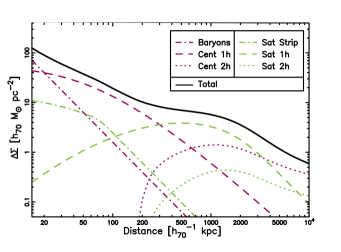
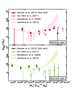
Figure 8: Left panel: Example from [89] showing how the various components of the halo contribute to the model lensing signal in the case of a halo at $z=0.5$ with mass $M_{200}=10^{12}M_{\odot}$, a stellar mass of $5\times 10^{10}M_{\odot}$ and a satellite fraction $\alpha=0.2$. The purple lines indicate quantities that correspond to centrals and the green lines are for satellites. Right panel: Comparison of lensing mass as a function of stellar mass for four independent data sets (as indicated) from [89]. The top shows results for red lenses and the bottom shows results for blue lenses. The results agree fairly well, where we note that the exact splits between samples differ between studies, which might explain some of the difference.

The lensing signal around central galaxies consists of two components. First of all, the lensing signal from the halo the galaxy resides in. This signal, the 1-halo term $\gamma_{T,1h}^{\rm cen}$, dominates on small scales as is highlighted in Figure 7. On larger scales the contribution from neighboring halos becomes dominant, which is described by the 2-halo term $\gamma_{T,2h}^{\rm cen}$. The terms simply add to give the total signal from central galaxies. The calculation of the 1-halo term requires the adoption of a halo density profile, but the 2-halo term is more involved. It requires the power spectrum to account for the correlation between the central galaxy and the dark matter distribution in nearby halos (expressions can be found in e.g. [75, 76, 87]). The detailed outcome depends on how these terms are computed, but the overall principles are pretty much the same. The main difference is how one deals with the transition from the single halo to multiple halo signal. This is because the dark matter halos of nearby halos cannot overlap, and different approaches to account for this have been proposed. More work is needed to improve the predictions in this critical regime.

The lensing signal around satellite galaxies consists of three terms. The simplest is the signal from the sub-halo in which the galaxy resides, although the result, $\gamma_{T,trunc}^{\rm sat}$ depends on the adopted tidally stripped density profile. There is also a contribution arising from the central halo in which the galaxy is located. As the satellites are mis-centered, calculating $\gamma_{T,1h}^{\rm sat}$ involves the convolution of the halo density profile with the spatial distribution of satellites. The last term, which is relevant on large scales, is the contribution from neighboring haloes, $\gamma_{T,2h}^{\rm sat}$. These three terms are added to obtain the satellite signal.

The left panel of Figure 8 shows an example of the signal predicted by the halo model and the various components from [89]. In addition to the components introduced above, [89] include a point mass contribution from the stellar mass contained in the galaxies. The result shows that the resulting signal shows features, which can be used to establish the satellite fractions. The right panel of Figure 8 shows a comparison of four different measurements (from [20, 90, 76, 89]) where the lenses have been split into blue and red samples (although we note that the detailed splits differ between studies, causing some differences). The results agree fairly well, although there are differences at the high mass end. These measurements will improve dramatically thanks to larger surveys. Of particular interest is the possibility to probe the evolution of galaxy properties, which only now is becoming possible. These early results show that galaxy-galaxy lensing is an important complement to galaxy clustering and luminosity function studies to place observational constraints on models of galaxy formation.

5.2 Halo Shapes

In addition to a specific average density profile, numerical simulations of cold dark matter show that dark matter halos are triaxial, with a typical ellipticity, in projection, of $\sim 0.3$ (e.g., [91, 92, 93]). The inner regions are believed to be significantly affected by baryonic processes, and predictions are rather uncertain. On larger scales, which are best constrained by the simulations, although we note that [94] and Kazantzidis10 have argued that baryonic effects lead to more oblate halos at all radii, weak lensing provides a unique way to constrain the halo shapes.

Although the precision of galaxy-galaxy lensing measurements has improved dramatically over the past years, constraints on the halo shapes are more difficult to obtain. This is because we need to measure the azimuthal variation in the galaxy lensing signal. For a singular isothermal ellipsoid, [95] showed that the signal-to-noise ratio with which the azimuthal variation can be determined is proportional to the mean halo ellipticity, $\epsilon_{h}$, and the S/N of the (isotropic) galaxy-galaxy lensing signal:

$$(S/N)_{\rm ani}=\frac{0.15}{\sqrt{2}}{\left(\frac{\epsilon_{h}}{0.3}\right)}(S/N)_{\rm iso}.$$ (27)

Hence in this best-case scenario, the precision is an order of magnitude lower than that of the galaxy lensing signal itself. The signal-to-noise ratio is reduced further because the signal declines relatively quickly with distance from the lens for more realistic density profiles, such as the NFW model. Furthermore, the light distribution of the lens is used as the reference frame to measure the azimuthal variation and any misalignment between the halo and the light will reduce the expected signal.

The azimuthally averaged galaxy lensing signal is robust against biases in the correction for PSF anisotropy, but this is not the case for the measurement of halo shapes: an imperfect correction may lead to correlations in the shapes of the lens and the sources, which changes the signal, although the impact is fairly modest ([96]). Lensing by structures at lower redshift can also cause correlations in the shapes. These contributions to the signal can be suppressed by subtracting the cross-shear from the measurements ([97, 95]), but at the expense of another factor $\sqrt{2}$ reduction in S/N.

Several studies have attempted to measure this signal, but the results remain inconclusive. [96] claim to have detected an alignment between the light distribution and the lensing signal through a maximum likelihood analysis of their data. These results are in agreement with the results from [98] who compared the tangential shear in quadrants. However, [97] did not detect a signal for their full sample of SDSS lenses, but a tentative signal was observed for bright early type lenses. Similarly, [95] did not detect a significant anisotropy signal, even though they analyzed an area that was $\sim 20$ times larger than [96]. An open question is whether this difference is due to the use of the maximum likelihood approach by [96], which should be more sensitive to the signal, although the interpretation may be more difficult. Significant progress is only possible with the next generation of imaging surveys, with their reduced errors and photometric redshift information for the lenses and the sources.

6 Lensing by Large-Scale Structure

Thus far we examined how weak gravitational lensing can be used to study the dark matter halos of galaxies and clusters. Such studies provide new observational constraints on models of galaxy evolution and provide an important approach to calibrate cluster masses. However, perhaps the most prominent application is weak lensing by large-scale structure, commonly referred to as “cosmic shear”. Compared to the other applications it is more sensitive to observational biases. The desire to measure the cosmic shear signal with high accuracy is therefore driving much of the development in the field of weak lensing, which in turn benefits the other applications.

The cosmic shear signal is a direct measure of the projected matter power spectrum, which simplifies the interpretation of the signal in principle, although we recall the aforementioned intrinsic alignments. Furthermore, as we discuss in §6.2 the predictions for the matter power spectrum remain uncertain. Nonetheless cosmic shear is considered one of the most powerful probes to study the distribution and growth of large-scale structure in the Universe. Since the first detections, reported in early 2000 ([99, 100, 101, 102]), the statistical power of the surveys has increased exponentially. We present some of the recent results from the Canada-France-Hawaii Telescope Legacy Survey (CFHTLS) in §6.3, but note that new surveys, which are an order of magnitude larger, are already underway. Importantly, the promise of weak lensing as a key cosmological probe was recognized by the European Space Agency with the selection of Euclid ([103]), scheduled for launch in 2020.

In the case of lensing by large-scale structure the deflection of light rays is not caused by a single deflector, but rather by all the inhomogeneities between the source and the observer. Here we only discuss the essentials and refer the interested reader to more detailed discussions in [3] or [5]. Recent reviews of the cosmological applications of weak lensing can be found in [104] and [105].

We assume that each deflection is small. Consequently, the distortion can be approximated by the integral along the unperturbed light ray rather than the actual path. This so-called Born approximation has been compared to full ray-tracing calculations and is found to be accurate to a few percent and allows us to define a deflection potential for a source at radial distance $\chi$ analogous to the thin-lens case:

$$\Psi({\bf x},\chi)=\frac{2}{c^{2}}\int_{0}^{\chi}{\rm d}\chi^{\prime}\frac{f_{K}(\chi-\chi^{\prime})}{f_{K}(\chi)f_{K}(\chi^{\prime})}\Phi(f_{K}(\chi^{\prime}){\bf x},\chi^{\prime}),$$ (28)

where the integral is over the lens coordinates $\chi^{\prime}$ and $f_{K}(\chi)$ indicates the angular diameter distances. The convergence and shear can be computed from this potential, just as for the single lens plane case. The use of the 3D Poisson equation in co-moving coordinates allows us to relate an overdensity $\delta$ to $\nabla^{2}\Phi$ as

$$\nabla^{2}\Phi=\frac{3H_{0}^{2}\Omega_{m}}{2a}\delta,$$ (29)

where $a$ is the scale factor. This allows us to compute the convergence $\kappa({\bf x},\chi)$:

$$\kappa({\bf x},\chi)=\frac{3H_{0}^{2}\Omega_{m}}{2c^{2}}\int_{0}^{\chi}{\rm d}\chi^{\prime}\frac{f_{K}(\chi-\chi^{\prime})f_{K}(\chi^{\prime})}{f_{K}(\chi)}\frac{\delta(f_{K}(\chi^{\prime}){\bf x},\chi^{\prime})}{a(\chi^{\prime})}.$$ (30)

If we consider an ensemble of sources with a redshift distribution $n(z){\rm d}z=p(\chi){\rm d}\chi$ the effective convergence is given by

$$\kappa({\bf x})=\int_{0}^{\chi_{\rm max}}{\rm d}\chi p(\chi)\kappa({\bf x},\chi)=\frac{3H_{0}^{2}\Omega_{m}}{2c^{2}}\int_{0}^{\chi_{\rm max}}{\rm d}\chi^{\prime}g(\chi^{\prime})f_{K}(\chi^{\prime})\frac{\delta(f_{K}(\chi^{\prime}){\bf x},\chi^{\prime})}{a(\chi^{\prime})},$$ (31)

i.e., the contribution from each lens plane is weighed by the lens efficiency factor

$$g(\chi^{\prime})=\int_{\chi^{\prime}}^{\chi_{\rm max}}{\rm d}\chi p(\chi)\frac{f_{K}(\chi-\chi^{\prime})}{f_{K}(\chi)}.$$ (32)

We can now compute the convergence power spectrum that arises from the power spectrum of density fluctuations, which in turn is determined by the initial cosmological conditions that we wish to determine. The convergence power spectrum $P_{\kappa}(\ell)$ is given by (see e.g., [3, 5] for details):

$$P_{\kappa}(\ell)=\frac{9H_{0}^{4}\Omega_{m}^{2}}{4c^{4}}\int_{0}^{\chi_{\rm max}}{\rm d}\chi\frac{g^{2}(\chi)}{a^{2}(\chi)}P_{\delta}\left({\frac{\ell}{f_{K}(\chi)},\chi}\right).$$ (33)

One complication is the fact that cosmic shear probes relatively small scales $(100<\ell<5000)$ where density fluctuations are non-linear. As a consequence, the power spectrum on those scales cannot be computed directly, but instead needs to be inferred from numerical simulations. We revisit this issue in §6.2.

So far we have only discussed the two-point statistics of the convergence field. However, as we show below the shear power spectrum is the same as that of the convergence (in the flat sky approximation). There is nonetheless a small complication because we cannot measure the shear, but only the reduced shear $g$ (see §2.4). Hence the relation between the observables and the underlying convergence field is more involved, but ray-tracing through cosmological simulations allow us to compute the necessary corrections (e.g., [106]).

To demonstrate that the shear and convergence power spectra are identical, we express the Fourier transforms of the convergence and shear in terms of the deflection potential (recall that a derivative $\partial/\partial x_{j}$ in real space corresponds to a multiplication by $-i\ell_{j}$ in Fourier space). Hence the Fourier transforms of the convergence, $\hat{\kappa}(\ell)$ and the shear $\hat{\gamma}(\ell)$ are given by

$$\hat{\kappa}(\ell)=-\frac{\ell^{2}}{2}\hat{\Psi}(\ell),~{}{\rm and}~{}\hat{\gamma}(\ell)=-\frac{\ell_{1}^{2}-\ell_{2}^{2}+2i\ell_{1}\ell_{2}}{2}\hat{\Psi}(\ell),$$ (34)

which once more shows that the shear and convergence are related (cf. Eqns 13 and 14):

$$\hat{\gamma}(\ell)=\frac{\ell_{1}^{2}-\ell_{2}^{2}+2i\ell_{1}\ell_{2}}{\ell^{2}}\hat{\kappa}(\ell)=e^{2i\phi}\hat{\kappa}(\ell),$$ (35)

which implies that

$$\langle\gamma(\ell)\gamma^{*}(\ell^{\prime})\rangle=\langle\kappa(\ell)\kappa^{*}(\ell^{\prime})\rangle=(2\pi)^{2}\delta(\ell-\ell^{\prime})P_{\kappa}(\ell).$$ (36)

In practice the situation is more complicated, because shapes cannot be measured reliably at every position. In particular bright stars saturate the detector, causing blooming and bleeding trails. Furthermore reflections in the optics give rise to halos and scattered light, which may prevent accurate measurements in some areas. As a result the actual survey geometry can be very complicated. This is very relevant as the holes created by bright stars have sizes of $\sim$ arcminutes, the scale where cosmic shear is most sensitive. Such a mask leads to the mixing of modes and therefore the observed power spectrum needs to be corrected, which increases the uncertainties further.

Alternatively one can consider other two-point statistics to quantify the cosmic shear signal. Of particular interest is the ellipticity correlation function, because it can be computed directly from a catalog of objects with shape measurements, and is insensitive to the mask. The mask, however, does change the number of pairs at certain distances, and thus the measurement errors. This does still complicate the calculation of the covariance matrix which is needed to interpret the cosmological nature of the signal.

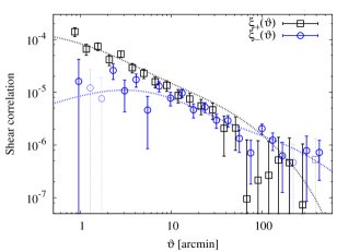
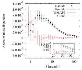
Figure 9: Left panel: Ellipticity correlation functions $\xi_{+}$ and $\xi_{-}$ measured by CFHTLenS from [107]. The dashed lines indicate the predictions for a WMAP7 cosmology. Right panel: Aperture mass variance from [107] which shows the E-mode in black and the B-mode in red. The latter is consistent with 0, suggesting that (additive) systematics have been removed successfully.

Although one could simply compute the correlation functions of the two shear component $\gamma_{1}$ and $\gamma_{2}$, it is more convenient to compute the correlation between the tangential $(\gamma_{T})$ and cross $(\gamma_{\times})$ components with respect to the line connecting a pair of galaxies and combine them into $\xi_{+}(\theta)$ and $\xi_{-}(\theta)$, defined as:

$$\xi_{\pm}(\theta)=\langle\gamma_{T}(\theta_{1})\gamma_{T}(\theta_{2})\rangle\pm\langle\gamma_{\times}(\theta_{1})\gamma_{\times}(\theta_{2})\rangle,$$ (37)

where $\theta=|\theta_{1}-\theta_{2}|$, hence the ensemble average depends only on the angular separation between the sources. The left panel in Figure 9 shows measurements for the ellipticity correlation functions by [107] from the weak lensing analysis of CFHTLS data by CFHTLenS, which is discussed in more detail in §6.3. For reference, predictions for a WMAP7 cosmology are also indicated. These can be computed from the convergence power spectrum because

$$\xi_{+/-}(\theta)=\frac{1}{2\pi}\int_{0}^{\infty}{\rm d}\ell J_{0/4}(\ell\theta)P_{\kappa}(\ell),$$ (38)

where $J_{i}$ is the $i-$th order Bessel function of the first kind. Note that the Bessel function does not vanish quickly, and consequently a large range in $\ell$ contributes to the correlation function at a given scale $\theta$.

The shear field is derived from the scalar deflection potential, which is a single (real) function of position. The fact that we measure two correlation functions implies there is redundancy in the data, as a single function should have sufficed. We use a similar argument in the case of mass reconstructions: in this case the imaginary part of the mass map does not arise from lensing, but from systematics (the same is true for the azimuthally averaged tangential shear). It is therefore useful to examine how such a separation can be done in the case of the cosmic shear signal. As the signal for over-(under)densities gives rise to a tangential (radial) shear pattern, analogous to the polarizations of the electric and magnetic field, the lensing induced signal is referred to as the ”E-mode”, whereas the cross component is given by the ”B-mode” ([108, 109]).

The derivation in [109] is particularly nice, as it clearly makes the link to the mass reconstruction case, and we refer the interested reader to this paper. It is possible to express E and B-mode power spectra in terms of the observed ellipticity correlation functions:

$$P_{E/B}(\ell)=\pi\int_{0}^{\infty}{\rm d}\theta\theta[\xi_{+}(\theta)J_{0}(\ell\theta)\pm\xi_{-}(\theta)J_{4}(\ell\theta)],$$ (39)

where the E-mode corresponds to the sum of the terms and the B-mode to the difference. It is also possible to separate the correlation functions themselves into $\xi_{E\pm}(\theta)$ and $\xi_{B\pm}(\theta)$, but as [109] point out, to compute these requires knowledge of $\xi_{-}(\theta)$ to arbitrarily large, and of $\xi_{+}(\theta)$ to arbitrarily small scales. This is not possible in the case of real data as neither can be observed. One solution is to account for this limited range in scales when predicting the signal, or instead using the model predictions to account for the lack of data.

This problem can be avoided by using aperture mass statistics, $\langle M_{\rm ap}^{2}\rangle(\theta)$, instead [110]. In this case the separation into E- and B-modes can be performed using correlation functions that extend to twice the scale of interest. Another advantage is that the smoothing of the convergence power spectrum is less severe. For this reason, cosmic shear studies often present results for the aperture masses. The right panel of Figure 9 shows the results for the CFHTLenS analysis from [107]. A clear E-mode signal is detected (black points), whereas the B-mode signal (red points) is consistent with 0, suggesting that (additive) systematics have been removed successfully.

In addition to the ellipticity correlation function and the aperture mass statistics, several other options have been proposed, either because of their ease of use, or because they allow for a cleaner E/B-mode separation. These are discussed in [107] who also provide expressions for their relation to the matter power spectrum.

6.1 Photometric redshifts and tomography

It is evident from Eqn. 33 that the cosmological interpretation of the cosmic shear signal requires accurate knowledge of the source redshifts. The lensing kernel in Eqn. 31, $g(\chi)f_{K}(\chi)$ (or $D_{L}D_{LS}/D_{S}$) peaks roughly halfway between the observer and the source, as can be seen from the left panel in Figure 10. The source redshift distribution, shown in the lower panel is described by

$$n(z)=n_{0}\frac{z^{a}}{z^{b}+c},$$ (40)

where $n_{0}$ is a normalization. For the results in Figure 10 we used $a=0.723$, $b=6.772$ and $c=2.282$, which yields a mean redshift of 0.85; this choice of parameters provides a good approximation for the redshift distribution of the CFHTLS data ([111]). The kernel is broad, and the lensing signal is sensitive to a large range in redshift. It does have the benefit that source redshifts need not be known with high precision: photometric redshifts are sufficient, although it is important that the mean is unbiased and the outlier fractions are known well. This avoids the need for spectroscopic redshifts for the individual sources, but note that the sources are very faint, which pushes the determination of photometric redshifts to the limits. Reliable measurements require good photometry in multiple bands and it is therefore important to correct for differences in the data quality [31].

Nonetheless large samples of galaxies with spectroscopic redshifts are needed to train and calibrate photometric redshift algorithms. This is because biases in the mean and higher order moments of the redshift distributions directly lead to biases in the inferred cosmological parameters. This is particularly critical for future projects. [112] provide an excellent overview of the needs for dark energy experiments. This aspect of cosmic shear is arguably as important as the fidelity of shape measurement techniques, but has not been examined as thoroughly, perhaps largely due to the paucity of large spectroscopic surveys. This is, however, changing rapidly and several approaches to improve photometric redshift estimates are being explored.

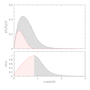
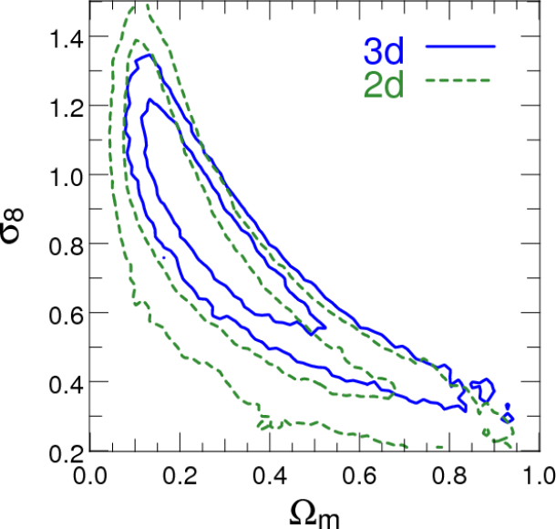
Figure 10: Left panel: The lensing kernel $g(\chi)f_{K}(\chi)$ as a function of lens redshift for the source redshift distributions shown in the bottom panel (see text for details.) Even though the sources have been split into a low ($z<0.85$) and high redshift bin $(z>0.85)$ as indicated, the lensing kernels overlap. Right panel: Constraints on $\Omega_{m}$ and $\sigma_{8}$ from [113]. The green contours show the results when the individual source redshifts are not used, whereas the blue contours show the results from a tomographic analysis. Although an improvement can be observed, the gain is limited because of cosmic variance due to the limited area covered by the 2 deg² COSMOS survey

The first cosmic shear results were based on observations in a single filter and the interpretation relied on redshift distributions obtained from deeper data ([50, 114]), but current surveys obtain multi-color data. Both the Deep Lens Survey (DLS; [55]) and CFHTLenS ([56]) use observations in five optical bands, which allowed them to determine photometric redshifts for individual sources. This not only helps the interpretation of the signal, but it also allows for the study of the lensing signal as a function of source redshift. Rather than considering the full redshift distribution, one can define redshift bins and compute the corresponding lensing signal, as well as cross correlations between bins. As first shown in [115] this cosmic shear tomography greatly improves the statistical power of a survey. The right panel of Figure 10 shows the results from the analysis of the 2 deg² COSMOS survey by [113]. An improvement in the constraints can be seen, although the results are limited by cosmic variance due to the relatively small survey area. A consequence of the broad lensing kernel is that the lensing signals for the bins are highly correlated, and the statistical gain saturates quickly (see e.g., Figure 3 in [116]), and $\sim 5$ bins are sufficient. One does need to account for intrinsic alignments, which are more pronounced in the narrower tomographic redshift bins ([23]). The modeling of the intrinsic alignment signal as a function of redshift is therefore a reason to actually increase the number of bins for future projects (e.g. [28]).

6.2 Predictions for the matter power spectrum

In addition to accurate shape measurements and photometric redshift estimates, the cosmological interpretation of the lensing signal requires accurate predictions for the matter power spectrum. On the largest scales the linear power spectrum can be computed for a given set of initial conditions. Perturbation theory can be used to compute corrections due to structure growth (see, [117] for a review; also see [118]) with an accuracy of a per cent for $k<0.2~{}h~{}{\rm Mpc}^{-1}$ (e.g., [119, 120]), depending on redshift. This approach, however, breaks down as structures become too overdense, collapse and virialize.

Cosmic shear surveys, however, are most sensitive to structures that are much smaller, such as groups of galaxies, i.e. very non-linear structures. The signal-to-noise ratio of the cosmic shear signal peaks on angular scales of $5-10$ arcminutes, or physical scales of $\sim 1$ Mpc (see e.g., [121, 122]). Restricting the analysis to large scales does not necessarily solve the problem, because the observed two-point ellipticity correlation functions are still sensitive to small scale structures projected along the line-of-sight. This can be avoided using a full 3D cosmic shear analysis (see [123, 124] for details), but using only large scales increases the statistical uncertainties dramatically due to cosmic variance, and thus is not a viable solution. Therefore the non-linear power spectrum needs to be computed to optimally extract the cosmological information from the measurements.

Currently only N-body simulations allow us to capture non-linear structure formation. In principle this can be done with good accuracy, provided the simulations are started with adequate initial conditions, with a large simulation volume, good time stepping and high mass resolution. For instance, [125] obtained an accuracy of $\sim 1\%$ out to $k\sim 1~{}h~{}{\rm Mpc}^{-1}$ for a gravity-only simulation. N-body simulations have also been used to calibrate recipes that allow one to compute the matter power spectrum from the linear power spectrum, such as [126], or the popularhalofit from [127]. Although these methods were sufficient for the interpretation of early cosmic shear studies, given their accuracy of $5-10\%$, the next generation of projects require percent level accuracy. One way forward is to run a suite of cosmological simulations spanning a range of cosmological parameters. These can be used to create an emulator of the power spectrum. For instance [128] describe the “Coyote Universe”, which comprises nearly 1000 N-body simulations, which can be used to predict the non-linear power spectrum out to $k\sim 1~{}h~{}{\rm Mpc}^{-1}$.

Another complication is that to infer cosmological parameters using a maximum likelihood method requires a covariance matrix. The non-linear growth of structure leads to correlations between scales, and the resulting mode coupling moves information from lower order moments of the density field to higher order moments. As a result the covariance matrix is not diagonal and the information content of two-point statistics is reduced (e.g. [129, 130]). Hence large numbers of numerical simulations are required for precise estimates of the covariance, in order to avoid biases in its inversion ([131]).

Thus far we only discussed N-body simulations, in which only gravity acts on the collisionless particles. This greatly simplifies the problem and allows for efficient calculations with high mass resolution over large volumes (e.g. [132, 133]). Although most of the matter in the Universe is indeed believed to be in the form of collisionless cold dark matter, baryons still represent about 17 percent of the total matter content. The distribution of baryons largely follows the underlying dark matter density field, and thus the results from N-body simulations should resemble the matter power spectrum fairly well. Nonetheless, differences in the spatial distribution of baryons with respect to the dark matter may result in significant changes (i.e. more than a few percent) in the actual matter power spectrum.

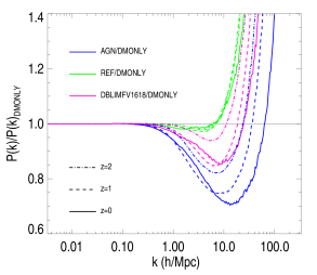
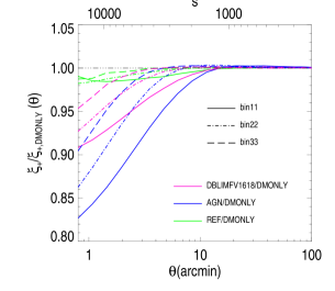
Figure 11: Left panel: Ratio of the power spectrum for different feedback models and the dark matter only case for three different redshifts from [122] based on the results from [134]. Of these models the AGN (blue curves) matches observations best. Right panel: The resulting change in the ellipticity correlation function $\xi_{+}$ for three redshift bins (0-0.6; 0.6-1.2;1.2-3.4), which is significant on scales where the cosmic shear S/N ratio is maximal ($s\sim$ few arcminutes). Ignoring the effects of baryon physics will therefore lead to biased cosmological parameter estimates.

Hence an accurate prediction for the matter power spectrum should include baryon physics. Various physical processes affect the distribution of baryons, such as radiative cooling, star formation and feedback from supernovae and active galactic nuclei (AGN). Prescriptions for these processes can be implemented in cosmological hydrodynamic simulations. As such simulations are much more expensive than N-body simulations, it has only recently become possible to simulate interesting cosmological volumes with reasonable resolution. It is, however, not clear which processes need to be included to reproduce observations. For this reason the accuracy of the results from hydrodynamic simulations is still under discussion, although we note that some recent simulations appear to match several key observables quite well ([135]).

The OverWhelmingly Large Simulations project (OWLS; [136]) produced a large number of simulations where various parameters that govern the feedback processes were varied. [134] used these results to examine the impact on the matter power spectrum. They found that different feedback processes can lead to rather large changes in the results. These results were used by [122] to examine the impact on cosmic shear studies and the left panel of Figure 11 shows the ratio of the matter power spectrum and the dark matter only results. The AGN model has the strongest feedback and leads to a suppression of $\sim 10\%$ at $k\sim 1~{}h~{}$Mpc^-1, but is also believed to match observations best ([135]). The right panel shows the corresponding change in the ellipticity correlation function $\xi_{+}(\theta)$, which is substantial on scales of a few arcminutes. The left panel of Figure 12 shows that the resulting cosmological parameter estimates are biased if baryon physics is ignored.

Our knowledge of the various feedback processes is still incomplete and we therefore cannot use these simulations to interpret the cosmic shear signal. Furthermore, hydrodynamic simulations are too expensive to compute covariance matrices, which would also be needed. Therefore several approaches have been suggested to parametrize our ignorance. [27] proposed to include an additional contribution, described by Legendre polynomials, to the power spectrum and marginalize over the nuisance parameters. A similar approach was suggested by [137]. These approaches reduce the statistical precision of a cosmic shear survey. Although one would like to obtain unbiased constraints on cosmological parameters, one should generally avoid reducing biases at the expense of precision. For instance [138] estimate that the degradation in dark energy constraints may be as much as $\sim 30\%$. Experiments are costly, and marginalizing over nuisance parameters should therefore be used as a last resort.

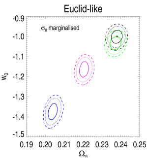
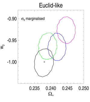
Figure 12: Left panel: Biases in recovered cosmological parameters (for a Euclid-like survey) for three different feedback models if the effects of baryon physics are ignored in the analysis (from [122]). The dot indicates the true parameter values. Right panel: The biases can be largely corrected for using a simple halo model that takes into account the different spatial distribution of baryons and dark matter.

Instead it is useful to examine whether it is possible to capture the effects of baryon physics on the matter power spectrum more effectively. [122] attempted to do so using a halo model approach, in which the baryons and stars were treated separately from the dark matter distribution: the distribution of stars were described by point masses, whereas the baryons followed a profile observed in X-ray observations. Importantly, feedback processes not only affect the power spectrum, but also affect scaling relations between halo mass and the stellar and gas mass. These can be observed, and thus used to constrain the halo model parameters. [122] fitted the simulated scaling relations and used the results to compute corrections to the dark matter power spectrum. The right panel in Figure 12 shows that, in principle, this relatively simple approach can reduce the biases in cosmological parameters significantly.

So far we have discussed only two-point statistics, mainly because those have been measured with high precision, and because the interpretation is relatively straightforward. However, as mentioned above, structure formation increases the power of higher order moments, and thus additional information can be extracted from e.g., the bispectrum (three-point statistics). For instance, the measurement of the three-point cosmic shear signal can break degeneracies between cosmological parameters (e.g. [12, 139, 140]), and a first reliable detection of the signal was reported in [141].

Compared to second-order statistics, higher-order statistics probe even smaller scales. Hence, baryon physics is expected to be more relevant. This was investigated by [142], who showed that this is indeed the case. Interestingly, [142] found that feedback affects the two- and three-point signal differently, opening up the possibility of testing the fidelity of the adopted feedback model by requiring consistency. The combination of second- and third-order statistics can also reduce the sensitivity to multiplicative biases, as was explored in [143]. Despite this promise, relatively little work is has been done to improve predictions for the bispectrum.

6.3 Results from CFHTLenS

Since the first reported detections of the cosmic shear signal, the surveyed areas have increased dramatically in size. The signal-to-noise ratio with which the signal can be measured has been increasing exponentially, and is projected to do so for another decade. Importantly, much effort has been spent on reducing and correcting for systematic errors. Another important development has been the availability of photometric redshift information for the sources, thanks to multi-color data.

We discuss future developments next, but in this section we highlight some results from the CFHTLenS team[56], who analysed the CFHTLS data. This survey was a large project to image 154 deg² in five optical filters with the CFHT. The survey comprises of four fields that range in area from $23-64$ deg². Thanks to the queue scheduling of CFHT the image quality in the $i^{\prime}-$band used for the lensing analysis is excellent. Nonetheless dealing with the various systematics has proven challenging. The data are presented in [144] and the lensing analysis is described in detail in [56], including the various tests that were performed. The resulting catalogs are publicly available from http://cfhtlens.org. Importantly, the analysis was done in a way that is blind to the cosmological parameters in order to avoid confirmation bias. Image simulations were used to calibrate the shape measurement algorithm lensfit, described in [43].

The resulting ellipticity correlation function from [107] was already shown in Figure 9, with a B-mode signal consistent with zero. The large area covered by the survey allows for a unique reconstruction of the large-scale mass distribution. These results are presented in [38] and showed a nice correlation between the peaks (and throughs) of the matter distribution and the light distribution. Some of the galaxy-galaxy lensing results were already discussed in §5.

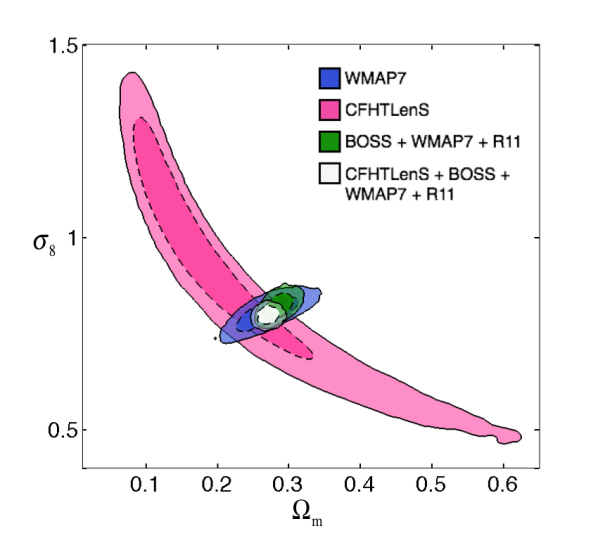
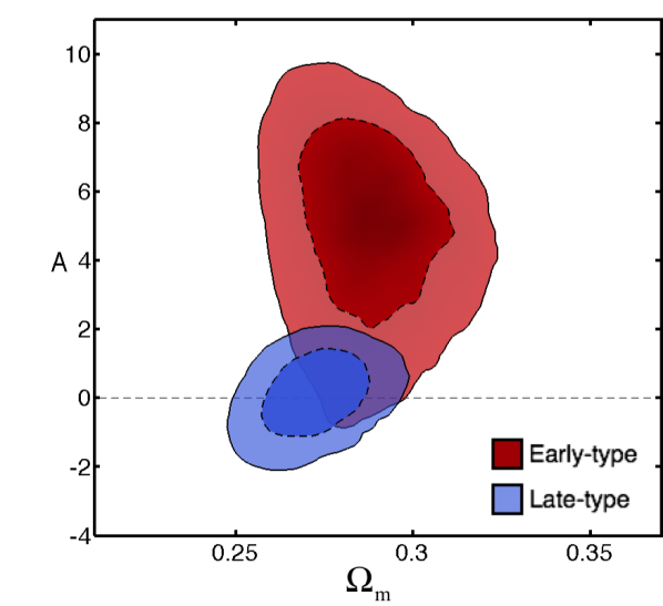
Figure 13: Left panel: Joint constraints on $\Omega_{m}$ and $\sigma_{8}$ from a tomographic weak lensing analysis by CFHTLenS (from [23]). The analysis accounted for the contamination by intrinsic alignments by adopting a simple alignment model, for which the amplitude was a free parameter. Right panel: The constraints on the amplitude of the intrinsic alignment signal and $\Omega_{m}$ for early- and late-type galaxies. A significant signal is measured for the former (from [23]).

The determination of the photometric redshifts is described in [145], who showed that the results are reliable in the range $0.2<z_{\rm phot}<1.3$, with a scatter after outlier rejection (the outlier rate is less than 10%) of $0.03<\sigma_{z}/(1+z)<0.06$. The fidelity of the redshift probability distribution functions was examined in [146] using measurements of the angular correlation function between bins in photometric redshifts. If the true redshifts of the bins do not overlap, then no significant correlation function should be observed (magnification could introduce a small signal though). Comparison of the clustering signal with that expected from the summed photometric redshift probability distributions showed good agreement.

[146] determined constraints on $\Omega_{m}$ and $\sigma_{8}$ by splitting the source samples into two broad redshift bins. This allowed them to ignore the spurious signal caused by intrinsic alignments. A more finely binned tomographic analysis, with the sources sorted into six redshift bins, was presented in [23]. For such narrow bins, intrinsic alignments start to contribute to the observed ellipticity correlation functions. To account for this [23] adopted a simple alignment model and determined the amplitude of the contaminating signal. The resulting constraints on $\Omega_{m}$ and $\sigma_{8}$ are reproduced in the left panel of Figure 13. The right panel shows the constraints on the amplitude of the alignment signal and $\Omega_{m}$. [23] found that the intrinsic alignment signal depends on galaxy type: for late-type galaxies the amplitude was found to be consistent with zero, but a significant signal was obtained for early type galaxies. Another nice application was presented in [147], who compared the cosmic shear results to measurements from the WiggleZ redshift survey ([148]) to observationally test modified gravity models. No deviation from general relativity was observed, but we note that statistical uncertainties are large. Nonetheless this study demonstrated the complementarity of cosmic shear surveys with redshift surveys, and the potential for future projects, which we will discuss next.

7 Outlook & Conclusions

The results from the CFHTLenS have demonstrated the potential of weak gravitational lensing to study the properties of dark matter halos around galaxies and to constrain cosmological parameters (also see [149, 55] for results from the Deep Lens Survey). The small survey area limited the precision of the constraints, but did provide an invaluable testbed to prepare for the next generation of surveys, which have already started taking data.

Of these, the Kilo Degree Survey (KiDS) started observations in 2012 with an anticipated completion of the 1500 deg² survey in 2016. Importantly the combination of excellent image quality and 9-band photometry, including sufficiently deep NIR data allows for the determination of good photometric redshifts. The Dark Energy Survey (DES) started in 2013 and will image 5000 deg², some of which will overlap with KiDS. Finally the new HyperSuprimeCam on Subaru will be used to image 1500 deg², but significantly deeper than the other two. Although the image quality of Subaru is excellent, the PSF is still too large to make optimal use of the additional galaxies, that will be mostly unresolved.

These projects will survey areas that are an order of magnitude larger than the CFHTLS. However, to learn more about the nature of dark energy and to study deviations from General Relativity, even larger areas of sky need to be imaged, to greater depth. From the ground the Large Synoptic Survey Telescope (LSST) is being developed. It will image the observable sky every week, and by combining the sharpest images into a deep stack, the weak lensing signal can be measured over more than 10,000 deg² (see [150] for an overview of the many science applications). It will, however, be challenging to model and correct the ground-based PSF sufficiently well to reach the statistical limit without significant biases.

The much smaller and stable PSF that can be achieved in space allows Euclid to measure the cosmic shear signal from two billion galaxies, surveying 15,000 deg², while observational biases are subdominant, as was shown in [103]. A detailed examination of the weak lensing design is presented in [151]. Thanks to its excellent image quality Euclid will also discover many strong lensing systems.

With a range of new surveys underway, or commencing very soon, the prospects for further progress in weak lensing are excellent. In these notes we touched upon the various applications, but also highlighted some of the key areas where further progress is needed. In particular we need to improve the modeling of the matter power spectrum as well as the bispectrum, develop a better understanding of intrinsic alignments and continue work on PSF modeling and shape measurement algorithms. Although they may be challenging, these all present excellent research opportunities.

- [1] \NAMEWalsh D., Carswell R. F. \atqueWeymann R. J., \INNature2791979381.
- [2] \NAMESoucail G., Fort B., Mellier Y. \atquePicat J. P., \INA&A1721987L14.
- [3] \NAMEBartelmann M. \atqueSchneider P., \INPhys. Rep.3402001291.
- [4] \NAMEBartelmann M., \INClassical and Quantum Gravity272010233001.
- [5] \NAMESchneider P., \TITLEPart 3: Weak gravitational lensing, in proc. of \TITLESaas-Fee Advanced Course 33: Gravitational Lensing: Strong, Weak and Micro, edited by \NAMEG. Meylan, P. Jetzer, P. North, P. Schneider, C. S. Kochanek, & J. Wambsganss 2006, pp. 269–451.
- [6] \NAMERefsdal S., \INMNRAS1281964307.
- [7] \NAMEKochanek C. S., \INApJ578200225.
- [8] \NAMESuyu S. H., Auger M. W., Hilbert S., Marshall P. J., Tewes M., Treu T., Fassnacht C. D., Koopmans L. V. E., Sluse D., Blandford R. D., Courbin F. \atqueMeylan G., \INApJ766201370.
- [9] \NAMESchneider P. \atqueSluse D., \INArXiv e-prints2013.
- [10] \NAMELewis A. \atqueChallinor A., \INPhys. Rep.42920061.
- [11] \NAMESeljak U., \INApJ46319961.
- [12] \NAMEBernardeau F., \INA&A324199715.
- [13] \NAMEvan Engelen A., Keisler R., Zahn O., Aird K. A., Benson B. A., Bleem L. E., Carlstrom J. E., Chang C. L., Cho H. M., Crawford T. M., Crites A. T., de Haan T., Dobbs M. A., Dudley J., George E. M., Halverson N. W., Holder G. P., Holzapfel W. L., Hoover S., Hou Z., Hrubes J. D., Joy M., Knox L., Lee A. T., Leitch E. M., Lueker M., Luong-Van D., McMahon J. J., Mehl J., Meyer S. S., Millea M., Mohr J. J., Montroy T. E., Natoli T., Padin S., Plagge T., Pryke C., Reichardt C. L., Ruhl J. E., Sayre J. T., Schaffer K. K., Shaw L., Shirokoff E., Spieler H. G., Staniszewski Z., Stark A. A., Story K., Vanderlinde K., Vieira J. D. \atqueWilliamson R., \INApJ7562012142.
- [14] \NAMEDas S., Sherwin B. D., Aguirre P., Appel J. W., Bond J. R., Carvalho C. S., Devlin M. J., Dunkley J., Dünner R., Essinger-Hileman T., Fowler J. W., Hajian A., Halpern M., Hasselfield M., Hincks A. D., Hlozek R., Huffenberger K. M., Hughes J. P., Irwin K. D., Klein J., Kosowsky A., Lupton R. H., Marriage T. A., Marsden D., Menanteau F., Moodley K., Niemack M. D., Nolta M. R., Page L. A., Parker L., Reese E. D., Schmitt B. L., Sehgal N., Sievers J., Spergel D. N., Staggs S. T., Swetz D. S., Switzer E. R., Thornton R., Visnjic K. \atqueWollack E., \INPhysical Review Letters1072011021301.
- [15] \NAMEPlanck Collaboration, Ade P. A. R., Aghanim N., Armitage-Caplan C., Arnaud M., Ashdown M., Atrio-Barandela F., Aumont J., Baccigalupi C., Banday A. J. \atqueet al., \INArXiv e-prints2013.
- [16] \NAMELeauthaud A., Massey R., Kneib J.-P., Rhodes J., Johnston D. E., Capak P., Heymans C., Ellis R. S., Koekemoer A. M., Le Fèvre O., Mellier Y., Réfrégier A., Robin A. C., Scoville N., Tasca L., Taylor J. E. \atqueVan Waerbeke L., \INApJS1722007219.
- [17] \NAMEBinggeli B., \INA&A1071982338.
- [18] \NAMECroft R. A. C. \atqueMetzler C. A., \INApJ5452000561.
- [19] \NAMEHeavens A., Refregier A. \atqueHeymans C., \INMNRAS3192000649.
- [20] \NAMEMandelbaum R., Hirata C. M., Ishak M., Seljak U. \atqueBrinkmann J., \INMNRAS3672006611.
- [21] \NAMEHirata C. M., Mandelbaum R., Ishak M., Seljak U., Nichol R., Pimbblet K. A., Ross N. P. \atqueWake D., \INMNRAS38120071197.
- [22] \NAMEJoachimi B., Mandelbaum R., Abdalla F. B. \atqueBridle S. L., \INA&A5272011A26.
- [23] \NAMEHeymans C., Grocutt E., Heavens A., Kilbinger M., Kitching T. D., Simpson F., Benjamin J., Erben T., Hildebrandt H., Hoekstra H., Mellier Y., Miller L., Van Waerbeke L., Brown M. L., Coupon J., Fu L., Harnois-Déraps J., Hudson M. J., Kuijken K., Rowe B., Schrabback T., Semboloni E., Vafaei S. \atqueVelander M., \INMNRAS43220132433.
- [24] \NAMEPereira M. J., Bryan G. L. \atqueGill S. P. D., \INApJ6722008825.
- [25] \NAMESchneider M. D., Cole S., Frenk C. S., Kelvin L., Mandelbaum R., Norberg P., Bland-Hawthorn J., Brough S., Driver S., Hopkins A., Liske J., Loveday J. \atqueRobotham A., \INMNRAS43320132727.
- [26] \NAMEHirata C. M. \atqueSeljak U., \INPhys. Rev. D702004063526.
- [27] \NAMEBernstein G. M., \INApJ6952009652.
- [28] \NAMEJoachimi B. \atqueBridle S. L., \INA&A5232010A1.
- [29] \NAMEHildebrandt H., van Waerbeke L. \atqueErben T., \INA&A5072009683.
- [30] \NAMEHildebrandt H., Muzzin A., Erben T., Hoekstra H., Kuijken K., Surace J., van Waerbeke L., Wilson G. \atqueYee H. K. C., \INApJ7332011L30.
- [31] \NAMEHildebrandt H., van Waerbeke L., Scott D., Béthermin M., Bock J., Clements D., Conley A., Cooray A., Dunlop J. S., Eales S., Erben T., Farrah D., Franceschini A., Glenn J., Halpern M., Heinis S., Ivison R. J., Marsden G., Oliver S. J., Page M. J., Pérez-Fournon I., Smith A. J., Rowan-Robinson M., Valtchanov I., van der Burg R. F. J., Vieira J. D., Viero M. \atqueWang L., \INMNRAS42920133230.
- [32] \NAMEKaiser N. \atqueSquires G., \INApJ4041993441.
- [33] \NAMEGorenstein M. V., Shapiro I. I. \atqueFalco E. E., \INApJ3271988693.
- [34] \NAMESeitz S. \atqueSchneider P., \INA&A3051996383.
- [35] \NAMESquires G. \atqueKaiser N., \INApJ473199665.
- [36] \NAMEBartelmann M., \INA&A3131996697.
- [37] \NAMESeitz S., Schneider P. \atqueBartelmann M., \INA&A3371998325.
- [38] \NAMEVan Waerbeke L., Benjamin J., Erben T., Heymans C., Hildebrandt H., Hoekstra H., Kitching T. D., Mellier Y., Miller L., Coupon J., Harnois-Déraps J., Fu L., Hudson M., Kilbinger M., Kuijken K., Rowe B., Schrabback T., Semboloni E., Vafaei S., van Uitert E. \atqueVelander M., \INMNRAS43320133373.
- [39] \NAMEHoekstra H., Franx M. \atqueKuijken K., \INApJ532200088.
- [40] \NAMEClowe D., Bradač M., Gonzalez A. H., Markevitch M., Randall S. W., Jones C. \atqueZaritsky D., \INApJ6482006L109.
- [41] \NAMEClowe D., Luppino G. A., Kaiser N., Henry J. P. \atqueGioia I. M., \INApJ4971998L61.
- [42] \NAMEMassey R., Hoekstra H., Kitching T., Rhodes J., Cropper M., Amiaux J., Harvey D., Mellier Y., Meneghetti M., Miller L., Paulin-Henriksson S., Pires S., Scaramella R. \atqueSchrabback T., \INMNRAS4292013661.
- [43] \NAMEMiller L., Heymans C., Kitching T. D., van Waerbeke L., Erben T., Hildebrandt H., Hoekstra H., Mellier Y., Rowe B. T. P., Coupon J., Dietrich J. P., Fu L., Harnois-Déraps J., Hudson M. J., Kilbinger M., Kuijken K., Schrabback T., Semboloni E., Vafaei S. \atqueVelander M., \INMNRAS42920132858.
- [44] \NAMEZuntz J., Kacprzak T., Voigt L., Hirsch M., Rowe B. \atqueBridle S., \INMNRAS43420131604.
- [45] \NAMEBernstein G. M., \INMNRAS40620102793.
- [46] \NAMEKaiser N., Squires G. \atqueBroadhurst T., \INApJ4491995460.
- [47] \NAMEHeymans C., Van Waerbeke L., Bacon D., Berge J., Bernstein G., Bertin E., Bridle S., Brown M. L., Clowe D., Dahle H., Erben T., Gray M., Hetterscheidt M., Hoekstra H., Hudelot P., Jarvis M., Kuijken K., Margoniner V., Massey R., Mellier Y., Nakajima R., Refregier A., Rhodes J., Schrabback T. \atqueWittman D., \INMNRAS36820061323.
- [48] \NAMEAmara A. \atqueRéfrégier A., \INMNRAS38120071018.
- [49] \NAMESemboloni E., Hoekstra H., Huang Z., Cardone V. F., Cropper M., Joachimi B., Kitching T., Kuijken K., Lombardi M., Maoli R., Mellier Y., Miller L., Rhodes J., Scaramella R., Schrabback T. \atqueVelander M., \INMNRAS43220132385.
- [50] \NAMEHoekstra H., Yee H. K. C., Gladders M. D., Barrientos L. F., Hall P. B. \atqueInfante L., \INApJ572200255.
- [51] \NAMEHoekstra H., Mellier Y., van Waerbeke L., Semboloni E., Fu L., Hudson M. J., Parker L. C., Tereno I. \atqueBenabed K., \INApJ6472006116.
- [52] \NAMEHoekstra H., \INMNRAS34720041337.
- [53] \NAMEHamana T., Miyazaki S., Okura Y., Okamura T. \atqueFutamase T., \INArXiv e-prints2013.
- [54] \NAMESchechter P. L. \atqueLevinson R. S., \INPASP1232011812.
- [55] \NAMEJee M. J., Tyson J. A., Schneider M. D., Wittman D., Schmidt S. \atqueHilbert S., \INApJ765201374.
- [56] \NAMEHeymans C., Van Waerbeke L., Miller L., Erben T., Hildebrandt H., Hoekstra H., Kitching T. D., Mellier Y., Simon P., Bonnett C., Coupon J., Fu L., Harnois-D’eraps J., Hudson M. J., Kilbinger M., Kuijken K., Rowe B., Schrabback T., Semboloni E., van Uitert E., Vafaei S. \atqueVelander M., \INArXiv e-prints2012.
- [57] \NAMEMassey R., Heymans C., Bergé J., Bernstein G., Bridle S., Clowe D., Dahle H., Ellis R., Erben T., Hetterscheidt M., High F. W., Hirata C., Hoekstra H., Hudelot P., Jarvis M., Johnston D., Kuijken K., Margoniner V., Mandelbaum R., Mellier Y., Nakajima R., Paulin-Henriksson S., Peeples M., Roat C., Refregier A., Rhodes J., Schrabback T., Schirmer M., Seljak U., Semboloni E. \atquevan Waerbeke L., \INMNRAS376200713.
- [58] \NAMEBridle S., Balan S. T., Bethge M., Gentile M., Harmeling S., Heymans C., Hirsch M., Hosseini R., Jarvis M., Kirk D., Kitching T., Kuijken K., Lewis A., Paulin-Henriksson S., Schölkopf B., Velander M., Voigt L., Witherick D., Amara A., Bernstein G., Courbin F., Gill M., Heavens A., Mandelbaum R., Massey R., Moghaddam B., Rassat A., Réfrégier A., Rhodes J., Schrabback T., Shawe-Taylor J., Shmakova M., van Waerbeke L. \atqueWittman D., \INMNRAS40520102044.
- [59] \NAMEKitching T. D., Balan S. T., Bridle S., Cantale N., Courbin F., Eifler T., Gentile M., Gill M. S. S., Harmeling S., Heymans C., Hirsch M., Honscheid K., Kacprzak T., Kirkby D., Margala D., Massey R. J., Melchior P., Nurbaeva G., Patton K., Rhodes J., Rowe B. T. P., Taylor A. N., Tewes M., Viola M., Witherick D., Voigt L., Young J. \atqueZuntz J., \INMNRAS42320123163.
- [60] \NAMEMelchior P. \atqueViola M., \INMNRAS42420122757.
- [61] \NAMETyson J. A., Valdes F., Jarvis J. F. \atqueMills, Jr. A. P., \INApJ2811984L59.
- [62] \NAMETyson J. A., Wenk R. A. \atqueValdes F., \INApJ3491990L1.
- [63] \NAMEHoekstra H., Bartelmann M., Dahle H., Israel H., Limousin M. \atqueMeneghetti M., \INSpace Sci. Rev.177201375.
- [64] \NAMEMahdavi A., Hoekstra H., Babul A., Bildfell C., Jeltema T. \atqueHenry J. P., \INApJ7672013116.
- [65] \NAMELeauthaud A., Finoguenov A., Kneib J.-P., Taylor J. E., Massey R., Rhodes J., Ilbert O., Bundy K., Tinker J., George M. R., Capak P., Koekemoer A. M., Johnston D. E., Zhang Y.-Y., Cappelluti N., Ellis R. S., Elvis M., Giodini S., Heymans C., Le Fèvre O., Lilly S., McCracken H. J., Mellier Y., Réfrégier A., Salvato M., Scoville N., Smoot G., Tanaka M., Van Waerbeke L. \atqueWolk M., \INApJ709201097.
- [66] \NAMEHoekstra H., Mahdavi A., Babul A. \atqueBildfell C., \INArXiv e-prints2012.
- [67] \NAMEOkabe N., Takada M., Umetsu K., Futamase T. \atqueSmith G. P., \INPASJ622010811.
- [68] \NAMEOkabe N., Smith G. P., Umetsu K., Takada M. \atqueFutamase T., \INApJ7692013L35.
- [69] \NAMEApplegate D. E., von der Linden A., Kelly P. L., Allen M. T., Allen S. W., Burchat P. R., Burke D. L., Ebeling H., Mantz A. \atqueMorris R. G., \INArXiv e-prints2012.
- [70] \NAMEKravtsov A. V., Vikhlinin A. \atqueNagai D., \INApJ6502006128.
- [71] \NAMEJohnston D. E., Sheldon E. S., Wechsler R. H., Rozo E., Koester B. P., Frieman J. A., McKay T. A., Evrard A. E., Becker M. R. \atqueAnnis J., \INArXiv e-prints2007.
- [72] \NAMECourteau S., Cappellari M., de Jong R. S., Dutton A. A., Emsellem E., Hoekstra H., Koopmans L. V. E., Mamon G. A., Maraston C., Treu T. \atqueWidrow L. M., \INArXiv e-prints2013.
- [73] \NAMEBrainerd T. G., Blandford R. D. \atqueSmail I., \INApJ4661996623.
- [74] \NAMEMcKay T. A., Sheldon E. S., Racusin J., Fischer P., Seljak U., Stebbins A., Johnston D., Frieman J. A., Bahcall N., Brinkmann J., Csabai I., Fukugita M., Hennessy G. S., Ivezic Z., Lamb D. Q., Loveday J., Lupton R. H., Munn J. A., Nichol R. C., Pier J. R. \atqueYork D. G., \INArXiv Astrophysics e-prints2001.
- [75] \NAMEMandelbaum R., Hirata C. M., Seljak U., Guzik J., Padmanabhan N., Blake C., Blanton M. R., Lupton R. \atqueBrinkmann J., \INMNRAS36120051287.
- [76] \NAMEvan Uitert E., Hoekstra H., Velander M., Gilbank D. G., Gladders M. D. \atqueYee H. K. C., \INA&A5342011A14.
- [77] \NAMESchneider P. \atqueRix H.-W., \INApJ474199725.
- [78] \NAMEHoekstra H., Yee H. K. C. \atqueGladders M. D., \INApJ606200467.
- [79] \NAMEHoekstra H., Hsieh B. C., Yee H. K. C., Lin H. \atqueGladders M. D., \INApJ635200573.
- [80] \NAMEHoekstra H., van Waerbeke L., Gladders M. D., Mellier Y. \atqueYee H. K. C., \INApJ5772002604.
- [81] \NAMESheldon E. S., Johnston D. E., Frieman J. A., Scranton R., McKay T. A., Connolly A. J., Budavári T., Zehavi I., Bahcall N. A., Brinkmann J. \atqueFukugita M., \INAJ12720042544.
- [82] \NAMEReyes R., Mandelbaum R., Seljak U., Baldauf T., Gunn J. E., Lombriser L. \atqueSmith R. E., \INNature4642010256.
- [83] \NAMEGuzik J. \atqueSeljak U., \INMNRAS3212001439.
- [84] \NAMESeljak U., \INMNRAS3182000203.
- [85] \NAMECooray A. \atqueSheth R., \INPhys. Rep.37220021.
- [86] \NAMELimousin M., Kneib J. P., Bardeau S., Natarajan P., Czoske O., Smail I., Ebeling H. \atqueSmith G. P., \INA&A4612007881.
- [87] \NAMECacciato M., van Uitert E. \atqueHoekstra H., \INArXiv e-prints2013.
- [88] \NAMETasitsiomi A., Kravtsov A. V., Wechsler R. H. \atquePrimack J. R., \INApJ6142004533.
- [89] \NAMEVelander M., van Uitert E., Hoekstra H., Coupon J., Erben T., Heymans C., Hildebrandt H., Kitching T. D., Mellier Y., Miller L., Van Waerbeke L., Bonnett C., Fu L., Giodini S., Hudson M. J., Kuijken K., Rowe B., Schrabback T. \atqueSemboloni E., \INArXiv e-prints2013.
- [90] \NAMELeauthaud A., Tinker J., Bundy K., Behroozi P. S., Massey R., Rhodes J., George M. R., Kneib J.-P., Benson A., Wechsler R. H., Busha M. T., Capak P., Cortês M., Ilbert O., Koekemoer A. M., Le Fèvre O., Lilly S., McCracken H. J., Salvato M., Schrabback T., Scoville N., Smith T. \atqueTaylor J. E., \INApJ7442012159.
- [91] \NAMEDubinski J. \atqueCarlberg R. G., \INApJ3781991496.
- [92] \NAMEJing Y. P. \atqueSuto Y., \INApJ5742002538.
- [93] \NAMEHayashi E., Navarro J. F. \atqueSpringel V., \INMNRAS377200750.
- [94] \NAMEKazantzidis S., Kravtsov A. V., Zentner A. R., Allgood B., Nagai D. \atqueMoore B., \INApJ6112004L73.
- [95] \NAMEvan Uitert E., Hoekstra H., Schrabback T., Gilbank D. G., Gladders M. D. \atqueYee H. K. C., \INA&A5452012A71.
- [96] \NAMEHoekstra H., Yee H. K. C. \atqueGladders M. D., \INApJ606200467.
- [97] \NAMEMandelbaum R., Hirata C. M., Broderick T., Seljak U. \atqueBrinkmann J., \INMNRAS37020061008.
- [98] \NAMEParker L. C., Hoekstra H., Hudson M. J., van Waerbeke L. \atqueMellier Y., \INApJ669200721.
- [99] \NAMEBacon D. J., Refregier A. R. \atqueEllis R. S., \INMNRAS3182000625.
- [100] \NAMEKaiser N., Wilson G. \atqueLuppino G. A., \INArXiv Astrophysics e-prints2000.
- [101] \NAMEVan Waerbeke L., Mellier Y., Erben T., Cuillandre J. C., Bernardeau F., Maoli R., Bertin E., McCracken H. J., Le Fèvre O., Fort B., Dantel-Fort M., Jain B. \atqueSchneider P., \INA&A358200030.
- [102] \NAMEWittman D. M., Tyson J. A., Kirkman D., Dell’Antonio I. \atqueBernstein G., \INNature4052000143.
- [103] \NAMELaureijs R., Amiaux J., Arduini S., Auguères J. ., Brinchmann J., Cole R., Cropper M., Dabin C., Duvet L., Ealet A. \atqueet al., \INArXiv e-prints2011.
- [104] \NAMEHoekstra H. \atqueJain B., \INAnnual Review of Nuclear and Particle Science58200899.
- [105] \NAMEMunshi D., Valageas P., van Waerbeke L. \atqueHeavens A., \INPhys. Rep.462200867.
- [106] \NAMEHilbert S., Hartlap J., White S. D. M. \atqueSchneider P., \INA&A499200931.
- [107] \NAMEKilbinger M., Fu L., Heymans C., Simpson F., Benjamin J., Erben T., Harnois-Déraps J., Hoekstra H., Hildebrandt H., Kitching T. D., Mellier Y., Miller L., Van Waerbeke L., Benabed K., Bonnett C., Coupon J., Hudson M. J., Kuijken K., Rowe B., Schrabback T., Semboloni E., Vafaei S. \atqueVelander M., \INMNRAS43020132200.
- [108] \NAMECrittenden R. G., Natarajan P., Pen U.-L. \atqueTheuns T., \INApJ568200220.
- [109] \NAMESchneider P., van Waerbeke L. \atqueMellier Y., \INA&A3892002729.
- [110] \NAMESchneider P., van Waerbeke L., Jain B. \atqueKruse G., \INMNRAS2961998873.
- [111] \NAMEBenjamin J., Heymans C., Semboloni E., van Waerbeke L., Hoekstra H., Erben T., Gladders M. D., Hetterscheidt M., Mellier Y. \atqueYee H. K. C., \INMNRAS3812007702.
- [112] \NAMENewman J., Abate A., Abdalla F., Allam S., Allen S., Ansari R., Bailey S., Barkhouse W., Beers T., Blanton M., Brodwin M., Brownstein J., Brunner R., Carrasco-Kind M., Cervantes-Cota J., Chisari E., Colless M., Comparat J., Coupon J., Cheu E., Cunha C., de la Macorra A., Dell’Antonio I., Frye B., Gawiser E., Gehrels N., Grady K., Hagen A., Hall P., Hearin A., Hildebrandt H., Hirata C., Ho S., Honscheid K., Huterer D., Ivezic Z., Kneib J.-P., Kruk J., Lahav O., Mandelbaum R., Marshall J., Matthews D., Ménard B., Miquel R., Moniez M., Moos W., Moustakas J., Papovich C., Peacock J., Park C., Rhodes J., Ricol J., Sadeh I., Slozar A., Schmidt S., Stern D., Tyson T., von der Linden A., Wechsler R., Wood-Vasey W. \atqueZentner A., \INArXiv e-prints2013.
- [113] \NAMESchrabback T., Hartlap J., Joachimi B., Kilbinger M., Simon P., Benabed K., Bradač M., Eifler T., Erben T., Fassnacht C. D., High F. W., Hilbert S., Hildebrandt H., Hoekstra H., Kuijken K., Marshall P. J., Mellier Y., Morganson E., Schneider P., Semboloni E., van Waerbeke L. \atqueVelander M., \INA&A5162010A63.
- [114] \NAMEVan Waerbeke L., Mellier Y. \atqueHoekstra H., \INA&A429200575.
- [115] \NAMEHu W., \INApJ5221999L21.
- [116] \NAMEMa Z., Hu W. \atqueHuterer D., \INApJ636200621.
- [117] \NAMEBernardeau F., Colombi S., Gaztañaga E. \atqueScoccimarro R., \INPhys. Rep.36720021.
- [118] \NAMECrocce M. \atqueScoccimarro R., \INPhys. Rev. D732006063519.
- [119] \NAMECrocce M., Scoccimarro R. \atqueBernardeau F., \INMNRAS42720122537.
- [120] \NAMETaruya A., Bernardeau F., Nishimichi T. \atqueCodis S., \INPhys. Rev. D862012103528.
- [121] \NAMEHuterer D. \atqueTakada M., \INAstroparticle Physics232005369.
- [122] \NAMESemboloni E., Hoekstra H., Schaye J., van Daalen M. P. \atqueMcCarthy I. G., \INMNRAS41720112020.
- [123] \NAMECastro P. G., Heavens A. F. \atqueKitching T. D., \INPhys. Rev. D722005023516.
- [124] \NAMEKitching T. D., Heavens A. F. \atqueMiller L., \INMNRAS41320112923.
- [125] \NAMEHeitmann K., White M., Wagner C., Habib S. \atqueHigdon D., \INApJ7152010104.
- [126] \NAMEPeacock J. A. \atqueDodds S. J., \INMNRAS2801996L19.
- [127] \NAMESmith R. E., Peacock J. A., Jenkins A., White S. D. M., Frenk C. S., Pearce F. R., Thomas P. A., Efstathiou G. \atqueCouchman H. M. P., \INMNRAS34120031311.
- [128] \NAMELawrence E., Heitmann K., White M., Higdon D., Wagner C., Habib S. \atqueWilliams B., \INApJ71320101322.
- [129] \NAMESemboloni E., van Waerbeke L., Heymans C., Hamana T., Colombi S., White M. \atqueMellier Y., \INMNRAS3752007L6.
- [130] \NAMEKiessling A., Taylor A. N. \atqueHeavens A. F., \INMNRAS41620111045.
- [131] \NAMEHartlap J., Simon P. \atqueSchneider P., \INA&A4642007399.
- [132] \NAMESpringel V., White S. D. M., Jenkins A., Frenk C. S., Yoshida N., Gao L., Navarro J., Thacker R., Croton D., Helly J., Peacock J. A., Cole S., Thomas P., Couchman H., Evrard A., Colberg J. \atquePearce F., \INNature4352005629.
- [133] \NAMECrocce M., Fosalba P., Castander F. J. \atqueGaztañaga E., \INMNRAS40320101353.
- [134] \NAMEvan Daalen M. P., Schaye J., Booth C. M. \atqueDalla Vecchia C., \INMNRAS41520113649.
- [135] \NAMEMcCarthy I. G., Schaye J., Ponman T. J., Bower R. G., Booth C. M., Dalla Vecchia C., Crain R. A., Springel V., Theuns T. \atqueWiersma R. P. C., \INMNRAS4062010822.
- [136] \NAMESchaye J., Dalla Vecchia C., Booth C. M., Wiersma R. P. C., Theuns T., Haas M. R., Bertone S., Duffy A. R., McCarthy I. G. \atquevan de Voort F., \INMNRAS40220101536.
- [137] \NAMEKitching T. D. \atqueTaylor A. N., \INMNRAS41620111717.
- [138] \NAMEZentner A. R., Rudd D. H. \atqueHu W., \INPhys. Rev. D772008043507.
- [139] \NAMEvan Waerbeke L., Bernardeau F. \atqueMellier Y., \INA&A342199915.
- [140] \NAMEVafaei S., Lu T., van Waerbeke L., Semboloni E., Heymans C. \atquePen U.-L., \INAstroparticle Physics322010340.
- [141] \NAMESemboloni E., Schrabback T., van Waerbeke L., Vafaei S., Hartlap J. \atqueHilbert S., \INMNRAS4102011143.
- [142] \NAMESemboloni E., Hoekstra H. \atqueSchaye J., \INMNRAS4342013148.
- [143] \NAMEHuterer D., Takada M., Bernstein G. \atqueJain B., \INMNRAS3662006101.
- [144] \NAMEErben T., Hildebrandt H., Miller L., van Waerbeke L., Heymans C., Hoekstra H., Kitching T. D., Mellier Y., Benjamin J., Blake C., Bonnett C., Cordes O., Coupon J., Fu L., Gavazzi R., Gillis B., Grocutt E., Gwyn S. D. J., Holhjem K., Hudson M. J., Kilbinger M., Kuijken K., Milkeraitis M., Rowe B. T. P., Schrabback T., Semboloni E., Simon P., Smit M., Toader O., Vafaei S., van Uitert E. \atqueVelander M., \INMNRAS43320132545.
- [145] \NAMEHildebrandt H., Erben T., Kuijken K., van Waerbeke L., Heymans C., Coupon J., Benjamin J., Bonnett C., Fu L., Hoekstra H., Kitching T. D., Mellier Y., Miller L., Velander M., Hudson M. J., Rowe B. T. P., Schrabback T., Semboloni E. \atqueBenítez N., \INMNRAS42120122355.
- [146] \NAMEBenjamin J., Van Waerbeke L., Heymans C., Kilbinger M., Erben T., Hildebrandt H., Hoekstra H., Kitching T. D., Mellier Y., Miller L., Rowe B., Schrabback T., Simpson F., Coupon J., Fu L., Harnois-Déraps J., Hudson M. J., Kuijken K., Semboloni E., Vafaei S. \atqueVelander M., \INMNRAS43120131547.
- [147] \NAMESimpson F., Heymans C., Parkinson D., Blake C., Kilbinger M., Benjamin J., Erben T., Hildebrandt H., Hoekstra H., Kitching T. D., Mellier Y., Miller L., Van Waerbeke L., Coupon J., Fu L., Harnois-Déraps J., Hudson M. J., Kuijken K., Rowe B., Schrabback T., Semboloni E., Vafaei S. \atqueVelander M., \INMNRAS42920132249.
- [148] \NAMEBlake C., Brough S., Colless M., Contreras C., Couch W., Croom S., Croton D., Davis T. M., Drinkwater M. J., Forster K., Gilbank D., Gladders M., Glazebrook K., Jelliffe B., Jurek R. J., Li I.-h., Madore B., Martin D. C., Pimbblet K., Poole G. B., Pracy M., Sharp R., Wisnioski E., Woods D., Wyder T. K. \atqueYee H. K. C., \INMNRAS4252012405.
- [149] \NAMEChoi A., Tyson J. A., Morrison C. B., Jee M. J., Schmidt S. J., Margoniner V. E. \atqueWittman D. M., \INApJ7592012101.
- [150] \NAMELSST Science Collaboration, Abell P. A., Allison J., Anderson S. F., Andrew J. R., Angel J. R. P., Armus L., Arnett D., Asztalos S. J., Axelrod T. S. \atqueet al., \INArXiv e-prints2009.
- [151] \NAMECropper M., Hoekstra H., Kitching T., Massey R., Amiaux J., Miller L., Mellier Y., Rhodes J., Rowe B., Pires S., Saxton C. \atqueScaramella R., \INMNRAS43120133103.