Conductance fingerprint of Majorana fermions in the topological Kondo effect
Abstract
We consider an interacting nanowire/superconductor heterostructure attached to metallic leads. The device is described by an unusual low-energy model involving spin- conduction electrons coupled to a nonlocal spin- Kondo impurity built from Majorana fermions. The topological origin of the resulting Kondo effect is manifest in distinctive non-Fermi-liquid (NFL) behavior, and the existence of Majorana fermions in the device is demonstrated unambiguously by distinctive conductance lineshapes. We study the physics of the model in detail, using the numerical renormalization group, perturbative scaling and abelian bosonization. In particular, we calculate the full scaling curves for the differential conductance in AC and DC fields, onto which experimental data should collapse. Scattering t-matrices and thermodynamic quantities are also calculated, recovering asymptotes from conformal field theory. We show that the NFL physics is robust to asymmetric Majorana-lead couplings, and here we uncover a duality between strong and weak coupling. The NFL behavior is understood physically in terms of competing Kondo effects. The resulting frustration is relieved by inter-Majorana coupling which generates a second crossover to a regular Fermi liquid.
pacs:
71.10.hf, 73.21.la, 73.63.kvI Introduction
Majorana fermions in superconductor heterostructures are presently the most viable candidates for realizing non-Abelian anyons.Read and Green (2000); *kitaev2001unpaired; Fu and Kane (2008); *sau2010generic; *alicea2010majorana; *oreg2010helical These emergent objects are zero-energy modes bound to certain point defects, fractionalising the regular fermionic degrees of freedom. Individual Majoranas can be far apart from each other, so that fermionic modes reconstructed from pairs of Majoranas can be nonlocal in character.Alicea (2012); *BeeMajrev Qubits encoding the occupation of such modes are topologically protected from local perturbations, and in consequence could find important application within fault-tolerant quantum computation.Nayak et al. (2008)
Several proposals for realizing the Majorana paradigm are the subject of ongoing experimental study, including heterostructures involving semiconductor nanowires with strong spin-orbit coupling,Mourik et al. (2012); *das2012zero; *Deng2012; Rokhinson et al. (2012) and those using boundary modes of topological insulators.Williams et al. (2012); Knez et al. (2012) Much of this experimental work has focused on demonstrating the existence of Majoranas by detecting the zero-bias anomaly in tunneling conductance, predicted from theory.Law et al. (2009); *wimmer2011quantum; *Saucond; *pientka2012enhanced Despite suggestive observations however, unambiguous experimental verification remains elusive because zero-bias peaks can also result from non-Majorana sources.Bagrets and Altland (2012); *pikulin2012zero; *liu2012zero; *kells2012nz
Compelling evidence for the existence of Majorana fermions in controllable nanodevices should therefore go beyond a direct spectral measurement, probing instead the topological nature of nonlocal qubits. Most theoretical work in this direction relates to phenomena in non-interacting systems.Hassler et al. (2010); *Saunet; *alicea2011non; *vanheck2012coulomb; *vanheckflux2013 However, richer physics could be accessible in systems which can host emergent Majorana particles in the presence of strong interactions between the physical electrons.Béri and Cooper (2012); Fu (2010); Tsvelik (2013); *crampe2013quantum; Béri (2013); *Altland2013; *Zazunov2013
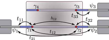
One such scenario was considered recently in Ref. Béri and Cooper, 2012: Majoranas at the end of nanowires on an interacting superconducting island produce several topological qubits (see Fig. 1). A spin- degree of freedom can be constructed from two such, which may be regarded as a nonlocal ‘quantum impurity’. Attaching metallic leads to the device allows this state to be probed by conductance measurement and, importantly, the spin of the nonlocal impurity is then flipped when an electron is transferred from one lead to the other. This gives rise to an effective exchange coupling between the spin- ‘impurity’ and the conduction electrons (which form a representation of spin-), resulting in a ‘topological Kondo effect’.Béri and Cooper (2012) The low-energy physics is controlled by renormalization group (RG) flow to an intermediate-coupling non-Fermi-liquid (NFL) fixed point,Béri and Cooper (2012) itself relatedFabrizio and Gogolin (1994); Fabrizio and Zarand (1996) to that of the four-channel Kondo (4CK) model.Nozières and Blandin (1980) This leads to distinctive signatures in physical properties, which could be used in experiment to identify clearly the topological Kondo effect, and hence the underlying existence of Majorana fermions in the device.
In this paper we examine this system in detail, going beyond the previous analysisBéri and Cooper (2012) to calculate the full temperature/energy dependence of physical quantities using the numerical renormalization group (NRG) technique.Bulla et al. (2008) We focus on the differential conductance in AC and DC fields, relevant to experiment. The lineshapes we obtain recover high- and low-energy asymptotes from CFT,Béri and Cooper (2012) but also contain new information on the entire crossover, which fundamentally encodes the RG flow. Experimental data collected on universal temperature/energy scales should collapse to a part of the full scaling curves presented in this paper, allowing experimental verification of the topological Kondo effect.
Our full NRG calculations also confirm a key prediction of Ref. Béri and Cooper, 2012 that the NFL physics is robust to asymmetric Majorana-lead couplings. This property has important implications for the practical viability of the setup, since fine-tuning is not required.
A rather complete picture of the complex physics of this system is obtained from analysis of its thermodynamics and scattering t-matrix. Characteristic properties of the NFL fixed point are found at low temperatures, including an unusual residual entropy for the Majoranas. Such behavior is similarly obtained at the NFL fixed point of the 4CK model;Andrei and Destri (1984); *Tsvelik1985 indeed, asymptotic corrections to fixed point thermodynamics of the form are common to both models. However, the entire crossover highlights differences, which uniquely fingerprint the topological Kondo effect. This is most clearly seen in the experimentally-relevant case of asymmetric Majorana-lead couplings: here the flow is distinct from that of the 4CK model. Furthermore, we uncover a duality between strong and weak coupling, allowing the Kondo scale at strong coupling to be obtained from simple perturbative scaling performed at weak coupling. In all cases, the NFL fixed point is reached at low energies—unlike the 4CK model, which supports a quantum phase transition to an unscreened local moment state.Schiller and De Leo (2008)
Finally, we consider relevant symmetry-breaking perturbations which do destabilize the NFL fixed point, generating a crossover to the conventional Fermi liquid state. Going beyond Ref. Béri and Cooper, 2012, we identify the coupling between different Majoranas to be one such perturbation. While such a coupling is expected to be very small (suppressed exponentially in the inter-Majorana separation), the resulting Fermi liquid crossover scale must in fact be much smaller than the Kondo scale in order that pristine NFL physics be observed at intermediate temperatures . In this case, we show that two successive universal crossovers arise: one to the NFL fixed point, and one away from it. Both crossovers are entirely characteristic of the incipient NFL state.
Given that the Kondo temperature may also be exponentially-small, a real device may have competing and scales. Here, conductance lineshapes obtained from NRG show more complex behavior, which depends on the ratio (a quantity that could be identified for a given experiment). But in all cases, Kondo-enhanced conductance establishes the existence of Majorana fermions in the device.
II Derivation of the model
We begin by reviewing how the topological Kondo effect arises.Béri and Cooper (2012) The main requirement for the Kondo effect is the coupling of conduction electrons to an impurity with a degenerate ground state. In the topological Kondo context, the impurity is constructed using a superconducting island with Majorana fermions (see Fig. 1). The island is of mesoscopic size, characterised by a charging term , where is the number operator for the island electrons and is the charging energy. The ground state will be degenerate if there are at least four Majoranas. Focusing on this minimal case (see also Fig. 1), if the Majorana wavefunctions do not overlap, each state with a given , and thus the ground state in particular, is twofold degenerate: the four Majoranas combine into two zero energy fermions with a fixed overall parity (their occupation can be changed only by transferring Cooper pairs to/from the superconducting condensate).Alicea (2012) It is this degeneracy that leads to an effective spin degeneracy for our Kondo model. If one includes the overlap of Majorana fermions and , the degeneracy is not exact: a “Zeeman” splitting that is exponentially small in the Majoranas’ separation arises, given by the term considered below.
The topological Kondo system is obtained by coupling the island to conduction electrons. In what follows, we focus on the minimal setup sketched in Fig. 1: we couple three of the four Majorana fermions to single-channel leads of effectively spinless conduction electrons (generated in practice by the application of a large magnetic field or spin-orbit couplingBéri and Cooper (2012)). The conduction electron spin densities, vital for any Kondo effect, will arise from nonlocal combinations of electron operators of different leads.Béri and Cooper (2012)
Working at energy scales much below the superconducting gap, and also much below the energies of any non-Majorana sub gap excitations, the physics is described by the Hamiltonian
| (1) |
where
| (2) |
| (3) |
| (4) |
and
| (5) |
Here is the Hamiltonian of conduction electrons, with creating scattering states (standing waves) of ingoing momentum in lead . The term describes the low energy coupling between the leads and the island. The operators correspond to localized conduction electron orbitals at the end of each physical wire,
| (6) |
and the phase exponential is also an operator, ensuring charge conservation by changing . To obtain , one expresses the electron operator on the island as [where are the Majorana wavefunctions and is the piece of the electron operator with positive energy BCS excitations], and writes down the usual hopping terms (where is the tunneling point in terms of the coordinates on the island). Below the energy scale of the superconducting gap, as discussed above, the piece can be neglected, which leads to Eq. 5.Fu (2010)
The key difference between the topological Kondo problem of Ref. Béri and Cooper, 2012 and Eq. (1) is that the former includes only the local couplings , while here we also consider the nonlocal and terms. Of course, due to the well-localized nature of the Majorana wavefunctions , these are exponentially suppressed with the inter-Majorana distance, . (We chose the phase of the electron operators so that .) At the lowest energy scales, as we will show, they will nevertheless lead to interesting, qualitatively new features.
On energy scales much lower than the charging energy , if one can simplify the model by a standard Schrieffer-Wolff transformation.Hewson (1997) Here it is convenient to assume that the charging term of is tuned to the middle of a Coulomb blockade valley111Moving away from the middle of the Coulomb blockade valley would generate non-universal (but RG-marginal) potential scattering terms in .Béri and Cooper (2012) We have checked numerically that that the non-Fermi-liquid fixed point discussed in Sec. III is robust to their inclusion; their effect on physical properties such as the finite-/finite- differential conductance is left for future work. where for some ; by considering virtual excitations to states of island charge , one obtains
| (7) |
in which repeated indices are summed over. (We add that type contributions are also generated by the couplings; these have been absorbed into the second term.)
Using now that the Majorana bilinears , and (the only independent ones due to the zero-mode parity constraint) form a spin- operator via
| (8) |
the effective model can be written in the form, . The conduction electron Hamiltonian is given in Eq. (3), and the Kondo coupling term isBéri and Cooper (2012)
| (9) |
where is a spin- operator for the lead electrons,
| (10) |
and the positive couplings . For , Eq. (9) can thus be viewed as an (anisotropic) Kondo model involving a spin- ‘impurity’ coupled to spin- conduction electrons.Fabrizio and Gogolin (1994); Béri and Cooper (2012)
Non-local couplings , , to leading order in exponentially small quantities, generate the term
| (11) |
Here are the five components of a spin-2 density where are elementary symmetric real matrices, and the real coupling constants are , and .
II.1 Simplification to the axial-symmetric limit
While the full model described by Eq. (9)–Eq. (11) can in principle be treated by the NRG (to be described later), the calculations are computationally rather expensive. There are two reasons for this: only the total charge is a conserved quantum number, and the Hamiltonian matrix has complex elements. The model as written also contains a large number of parameters, and one cannot hope to examine its full parameter space exhaustively.
We therefore adopt the following simplifications. For much of the paper, we focus on , to identify and understand the universal physics arising from the topological Kondo effect of Eq. (9). To simplify the calculations, we now assume , and imaginary . This leads to a residual ‘axial symmetry’ around axis , as will be discussed in due course, which allows the calculations to be performed with real matrix elements and exploiting the conservation of an additional, overall quantum number.
To obtain a handle on the key effects of the perturbation , one can focus on the non-local couplings arising from the exponentially small overlap between Majoranas and alone. This simplifies the model considerably, as it can then be shown that the first term in Eq. (11) is then absent. We leave a study of the more general case to future work; our expectation is that the remaining perturbations we keep in are sufficient to understand the essential effects of non-local couplings between the Majoranas: namely that if the non-local couplings are made sufficiently small, the universal non-Fermi-liquid physics of the model persists above a low-energy crossover scale set by the size of (see Sec. VI).
With these simplifications in place, we employ a unitary transformation of the lead operators to a basis labeled by the conduction electron spin projection, , viz,
| (12a) | ||||
| (12b) | ||||
| (12c) | ||||
The lead Hamiltonian then follows simply as . Localized orbitals in the new basis are defined as
| (13) |
in terms of which the spin- ladder operators of the lead electrons are
| (14a) | ||||
| (14b) | ||||
| (14c) | ||||
It is then straightforward to show that under the above transformation, the Kondo model including the perturbations takes the form 222If one takes , the coupling constants in Eq. (15) are simply related to those of Eq. (9) by , and . Non-local couplings generate the term and unequal , and then the relationship between the two sets of coupling constants becomes more complicated.
| (15) |
with and spin- operators for the ‘impurity’ as before.
The dependence of the four coupling constants in Eq. (15) on the original model parameters is generally non-trivial. Since the aim of this work is to examine the universal physics of the model and understand the basic effect of non-local couplings between Majoranas, we shall treat the coupling constants of Eq. (15) as the bare model parameters of interest. With this in mind, we make one final simplification: we set . Since a Zeeman term is associated with the same effective time-reversal symmetry breaking as setting , the basic effect of this symmetry breaking can be probed by considering the latter alone.
To calculate thermodynamic and dynamical properties of Eq. (15), we employ the NRG, a powerful non-perturbative method which yields numerically-exact results over a wide range of temperature/energy scales. The general procedure for calculating thermodynamics is explained fully in the review of Ref. Bulla et al., 2008, to which we refer the reader for further details.
The key approximation in NRG is a logarithmic discretization of the conduction electron densities of states. Since we focus on the universal physics of the model here, it suffices to consider equivalent symmetric bands, each with constant density of states over a bandwidth . These are discretized and transformed into semi-infinite 1d tight-binding ‘Wilson chains’,
| (16) |
where the impurity couples only to the ‘zero-orbital’ , as defined in Eq. (13). The logarithmic discretization means that the Wilson chain hoppings decrease exponentially down the chain, rendering the problem amenable to an iterative solution in which high-energy states are successively discarded as more Wilson chain orbitals are added.Bulla et al. (2008) Dynamics are calculated within the complete Anders-Schiller basis,Anders and Schiller (2005) using the ‘full density matrix’ approach.Weichselbaum and von Delft (2007); *Peters2006 In practice we exploit the symmetries of Eq. (15) (overall charge and conservation). We use a discretization parameter , and retain at most 10000 states at each iteration. The results of 8 separate calculations with different discretization ‘slide parameter’ are combined to obtain highly accurate dynamics.Oliveira and Oliveira (1994)
III Fixed points and symmetries
Before presenting numerical results, we first identify and discuss the fixed points of the model, Eq. (15), and consider the RG flows between them. We begin with the axial symmetric limit , where an intermediate coupling, non-Fermi-liquid fixed point is stable. Further insight into this fixed point can then be gained by considering the behavior of the model when : the intermediate coupling fixed point arises from a competition between two Kondo effects, as explained below.
At high energies, the physics of the model is controlled by the local moment (LM) fixed point, obtained by setting in Eq. (15). At the fixed point itself, the spin (the ‘impurity’) decouples from the three conduction electron channels, to giveHewson (1997) an ‘impurity entropy’ and Curie law magnetic susceptibility (we use units where and throughout). Near the fixed point, antiferromagnetic exchange coupling is (marginally) relevant, and its effect can be understood using Anderson’s poor man’s scalingAnderson (1970); Béri and Cooper (2012) (i.e. perturbative RG) to obtain flow equations for the renormalized couplings as the effective bandwidth/energy scale is reduced. Defining dimensionless running couplings , , and with the running UV cutoff, second-order poor man’s scaling gives
| (17) |
These equations are precisely those obtained for the spin- anisotropic Kondo model, with a single spinful conduction electron channel.Hewson (1997) The initial RG flow is therefore similar to that of the regular Kondo problem: weak antiferromagnetic bare couplings begin to grow as the temperature/energy scale is reduced, showing up in physical quantities such as the conduction electron t matrix and conductance as slow inverse-logarithmic tails at high energies.Hewson (1997); Dickens and Logan (2001)
In the antiferromagnetic one-channel Kondo problem, it is well knownHewson (1997) that RG flows tend ultimately to a stable, isotropic strong coupling (SC) fixed point, describing the Kondo singlet at very low energies. [This conclusion is naturally beyond the scope of the perturbative scaling analysis, but has been established by exact methods including NRGBulla et al. (2008) and the Bethe ansatz.Tsvelick and Wiegmann (1983); Andrei et al. (1983)] An isotropic SC fixed point also exists for Eq. (15), obtained by setting in Eq. (15) and in Eq. (16) (which decouples the three leads subject to a phase shift). But in contrast to the conventional Kondo model, this SC fixed point is unstable. The reason is that the decoupled subsystem comprising the impurity and the three ‘zero orbitals’ has degenerate ground states with local charge and , which are connected by a relevant perturbation of the form 333We noteKrishnamurthy et al. (1980) that the same perturbation connects degenerate charge states of the ‘free orbital’ fixed point in the regular Anderson impurity model
| (18) |
In the conventional Kondo model, there is no such internal structure at the SC fixed point: the strong coupling state is an ‘inert’ singlet and no such relevant perturbations around the fixed point are possible.
With both LM and SC fixed points unstable when , one anticipates the existence of a stable fixed point at intermediate coupling. This intermediate coupling fixed point was shown to be stable within a form of the Toulouse limit for a model with axial symmetry.Fabrizio and Gogolin (1994) A full CFTAffleck (1990); *affleck1991kondo; *affleck1991critical; *Affleck1993 analysis of the problem was recently performed,Béri and Cooper (2012) establishing that this overscreened NFL fixed point is robust to breaking exchange isotropy () or, equivalently, to asymmetries of the local couplings in the original model of Eq. (1).
Further insight into the model can be obtained by noting that the spin sector of the model, Eq. (15), is identical to that of the four-channel Kondo (4CK) model.Fabrizio and Gogolin (1994); Fabrizio and Zarand (1996); Sengupta and Kim (1996) The physics near the intermediate coupling fixed point therefore has many common features with that of the 4CK effect. The latter has been studied using the Bethe ansatzAndrei and Destri (1984); *Tsvelik1985 and boundary CFT,Affleck (1990) which predict for example a residual impurity entropy and NFL low-temperature behavior such as a divergent susceptibility . As these thermodynamic quantities originate from the spin sector, the same behavior is expected for the topological Kondo effect studied here. But crucially, the remaining sectors of the two models are distinct. The realization of the NFL fixed point with a spin- conduction band changes certain key physical properties, as we will illustrate through our calculation of the scattering -matrix (see Sec. IV.3). Moreover, although the fixed points of Eq. (15) and the 4CK model are similar, the RG flows between them are also quite different, as we shall discuss in Sec. V.
Upon including non-local couplings , we perturb the fixed point studied in Ref. Béri and Cooper, 2012 in an as-yet unexplored manner. These perturbations lead to qualitative changes: since they introduce complex couplings in Eq. (7), they break the effective time-reversal invarianceBéri and Cooper (2012) responsible for the stability of the NFL fixed point. But if these couplings are sufficiently small (see Sec. VI for a precise definition of ‘small’), the NFL behavior will persist down to an energy scale , before the symmetry-breaking becomes important and deviations occur.
In terms of the simplified model under consideration in this work, Eq. (15), the non-local couplings manifest themselves in two ways. As discussed in Sec. II, they introduce an effective magnetic field (neglected here, as explained in Sec. II.1) and they lead to . To understand the effect of the latter further, we can rewrite Eq. (15) as , with
| (19) | |||||
| (20) |
and . In this form the model has a simple physical interpretation. The terms and each describe a spin- anisotropic Kondo model, with spin- conduction electrons. In , channels and can be thought of as the ‘’ and ‘’ spins of a conventional Kondo model; while in these roles are played by channels and . Crucially, channel plays a different role in than it does in — it is therefore not possible to combine channels into a single ‘’ channel and have channel acting as the ‘’ spin in both terms (this is merely a statement that Kondo models with spin- and spin- conduction electrons are inequivalent).
When , then grows under renormalization faster than , and the system is driven to an isotropic strong coupling fixed point. The impurity spin- is exactly Kondo-screened by the and channels of , with . Meanwhile, the third channel, decouples, . By contrast, when , the Kondo effect takes place with the and channels, with now decoupling.
The critical physics of the model near can thus be understood physically in terms of competing Kondo effects in different channels, depending on whether . On tuning precisely to (i.e. ), one realizes the stable NFL fixed point of the model: by symmetry, neither nor can individually decouple, with the result that the impurity is ‘overscreened’. This competition between strong coupling Kondo-screened states, and the accompanying emergence of NFL physics, similarly arises in the multichannel KondoNozières and Blandin (1980); Mitchell et al. and multi-impurity KondoJones et al. (1988); *Jones1991; Affleck and Ludwig (1992); *Affleck1995; Mitchell et al. (2012, ) problems.
The quantum phase transition arising on tuning is explored further in Sec. VI.
IV NRG Results for the channel-isotropic limit
We begin by examining the physics when [i.e. equal local couplings, in Eq. (9)]. Here the model has full spin symmetry, with each screening channel coupled equivalently to the central impurity spin. As mentioned in Sec. III, our model Eq. (15) in this limit has the same NFL fixed point as the 4CK model, and is therefore expected to show similar low-energy physics.Fabrizio and Gogolin (1994); Fabrizio and Zarand (1996); Sengupta and Kim (1996) This is confirmed below. We also look beyond the low-energy regime, calculating exactly with NRG the full universal crossover behavior of the thermodynamics and dynamics.
IV.1 Thermodynamics
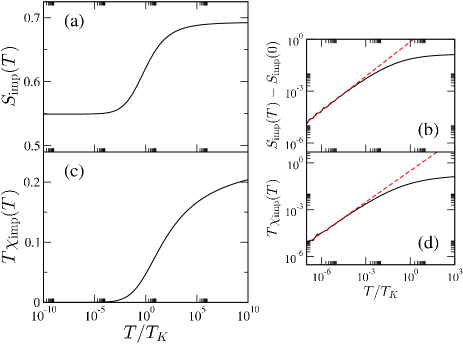
The RG flow associated with the isotropic model is seen most vividly in the ‘impurity entropy’ as a function of temperature, , defined as the difference in entropy between and . The Kondo temperature, , sets the scale for universal flow from the LM fixed point to the NFL fixed point. In practice, we define it numerically via , suitably halfway between the limiting fixed point entropies. Numerical results for any choice of the bare parameter then collapse onto a single universal scaling curve when plotted in terms of . This scaling curve is shown in Fig. 2(a).
The general form of the entropy scaling curve for the model Eq. (15) in the isotropic limit is indeed as one would expect for the 4CK model: a crossover on the scale of from the LM fixed point with to the NFL fixed point, with residual entropyAndrei and Destri (1984); *Tsvelik1985; Affleck (1990) (this non-trivial value is reproduced very accurately in our NRG calculations). Behavior in the vicinity of the fixed point is characteristic of the non-Fermi-liquid physics, with leading corrections in the low-temperature limit of , as shown in Fig. 2(b) by comparison to the dashed line. This behavior arises in the 4CK modelAndrei and Destri (1984); *Tsvelik1985; Affleck (1990) due to a leading irrelevant operator of scaling dimension . The leading irrelevant operator at the NFL fixed point of Eq. (9) was identified in Ref. Béri and Cooper, 2012, and has the same scaling dimension.
Figure 2(c) shows a similar universal plot of the impurity spin susceptibility vs . The low behavior [see Figure 2(d)] is found to be , again entirely consistent with 4CK-like physics.Andrei and Destri (1984); *Tsvelik1985; Affleck (1990)
IV.2 Kondo temperature
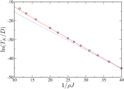
Having examined the universal thermodynamics as a function of , we now consider the dependence of the Kondo temperature, , on the coupling strength, . The asymptotic behaviour for small can be obtained by applying perturbative scalingAnderson (1970) to Eq. (15), which yields
| (21) |
to third-order. This result is tested and confirmed in Fig. 3, where we plot vs [points obtained by NRG, dashed line is Eq. (21)]. It is worth pointing out here that Eq. (21) is also obtained for the 4CK model from perturbative scaling, suggesting that the RG flow from the (same) LM to NFL fixed points in the two models are rather similar, at least for small .
For comparison, the second-order perturbative scaling result, , is plotted as the dotted line in Fig. 3. At this level one does not obtain the prefactor in front of the exponential in Eq. (21); from the figure it is clear that this prefactor has a rather strong influence on the Kondo scale for moderate values of .
IV.3 Scattering t-matrix
We turn now to the dynamics of the model Eq. (15), about which far less is currently known. Asymptotic behavior near the NFL fixed point of the 4CK model has been extracted using CFT,Affleck (1990); *affleck1991kondo; *affleck1991critical; *Affleck1993 but full crossover functions for either model have not previously been calculated.
The scattering t matrix is a central quantity of interest, which contains rich information about the RG flow and underlying physics. It describes scattering between eigenstates of the disconnected leads, induced by the ‘impurity’, and is thus defined for a given channel, , in terms of the retarded Green function for conduction electrons in that channel,
| (22) |
Equations of motionZubarev (1960) for the Fourier transformed Green function, , then yield directly
| (23) |
where is the Green function of the free leads in the absence of the impurity. is the t matrix, which contains information about electronic correlations and the Kondo effect. We consider its spectrum,
| (24) |
Note that, although is defined in terms of the lead operators in the rotated basis of Eq. (15), it also describes scattering in the physical basis of Eq. (9). This follows because the transformation Eq. (12b) is trivial for so that, from Eqns. (22)–(24), the t matrix of the physical lead is simply given by that for channel in the rotated basis. Then, channel isotropy implies that the t matrices for all physical and rotated channels are identical. In practice we calculate the single t matrix from with NRG. Details can be found in Appendix A.
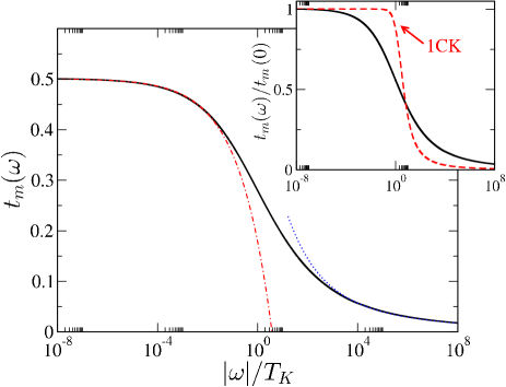
The universal RG flow between the LM and NFL fixed points is naturally reflected in the spectrum , the scaling curve for which we show in Fig. 4 in terms of (solid line obtained by NRG). The full crossover can be understood in terms two asymptotic limits. The high-frequency ‘tail’ in , obtained for , is associated with simple perturbative scattering of conduction electrons from the spin- impurity local moment. The resulting behavior of the spectrum (which is common to all problems in which local moment physics plays a key role), takes the formDickens and Logan (2001)
| (25) |
with and constants. A fit to this form is shown as the dotted line in Fig. 4, which our exact numerics approach asymptotically for . In the opposite regime , the t matrix has the characteristic behavior
| (26) |
with . This power-law form is as predicted by CFT: generally one expects , with the scaling dimension of the leading irrelevant operator near the stable fixed point; here, ,Béri and Cooper (2012) thus yielding Eq. (26). Excellent agreement between Eq. (26) (dot-dashed line in Fig. 4) and the exact NRG result is found over a wide range of energies.
As pointed out earlier, the -matrix exemplifies certain key differences between the low energy physics of the 4CK and the present model. This is seen immediately in the zero-frequency values: for the 4CK model, CFT predictsAffleck (1990) , while here it recovers the value observed in Fig. 4. This simply reflects the different forms of the conduction channels of the two models (four spin- channels versus one spin- channel); indeed, the result is correctly recovered using the CFT fusion rules of Ref. Affleck, 1990 with spin- conduction electrons.
The inset of Fig. 4 compares the universal scaling spectrum of the t matrix for Eq. (15) (solid line) to that known for the regular one-channel Kondo (1CK) model (dashed line), both plotted as for ease of comparison. 444For the 1CK model, ; and we define via . The two curves are strikingly different: the crossover from the high-frequency tails to the low-frequency power-law is much sharper in the 1CK case than for the present model. This is consistent with the very different leading corrections to the stable fixed points of the two models. Fermi-liquid theory for the 1CK model predictsHewson (1997) the ubiquitous quadratic approach to the Fermi level value, , as compared to the slower NFL corrections of Eq. (26).
IV.4 Linear conductance
Finally, we consider the zero-bias differential conductance — the central quantity of experimental relevance: measuring this simply amounts to measuring a current in one of the leads as a response to infinitesimally small voltages.
We employ the Kubo formalismIzumida et al. (1997) to obtain an expression amenable to treatment within NRG (see Appendix B for details). Our focus is the conductance in an AC field. As such, we assume that the system is in equilibrium at time , with all three leads at a common chemical potential . The chemical potential of lead is then given a time dependence , switched on adiabatically from . Denoting the total electronic number operator of lead by , the current flowing into lead has reached an oscillatory steady state by time . The dimensionless AC conductance tensor is then defined as
| (27) |
which holds at any temperature . On taking the limit one obtains the static conductance,
| (28) |
in response to a DC voltage switched on adiabatically from .
In the channel-isotropic limit under consideration in this section, the off-diagonal elements for are identical by symmetry. Moreover, as shown in Appendix B, they are related to the diagonal elements by
| (29) |
Physically, the minus sign reflects the fact that a positive bias applied to lead produces net current flow from lead to leads — i.e., positive current towards lead and negative current towards lead . The entire conductance tensor is thus fully determined by a single element; we calculate explicitly below.
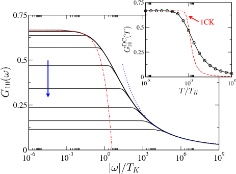
As one would expect from the preceding results, we find from NRG that is a universal function of at any given temperature . The main panel of Fig. 5 shows the scaling form of vs both at zero temperature, and for a range of temperatures with integral , increasing in the direction of the arrow.
As with the t matrix, the form of at can be understood in terms of its asymptotes. At high frequencies, one observes conductance signatures characteristic of spin-flip scattering of conduction electrons from an asymptotically-free impurity spin, again of the form
| (30) |
as confirmed by comparison to the dotted line in the main panel of Fig. 5. On the scale of , RG flow toward the NFL fixed point results in an enhancement of the conductance. At low frequencies , corrections to the NFL fixed point yield characteristic power-law behavior,
| (31) |
with . NRG results fold onto Eq. (31) for , as shown by comparison with the dot-dashed line in Fig. 5. 555NRG recovers the exact value to within a few percent (although numerical errors can in principle be systematically reduced). In our analysis of the low-frequency power-law behavior of , we therefore treated as a fitting parameter. A fit to the form extends to the lowest frequencies, compared with other simple rational powers. We note that the leading correction here is of the form — different from the behavior observed for the t matrix, see Eq. (26). This difference is understood by a simple extension of the CFT arguments given in Ref. Béri and Cooper, 2012: perturbation theory around the NFL fixed point in the leading irrelevant operator yields corrections to the conductance which vanish to first order, by symmetry. The expected behavior is thus replaced by leading second-order corrections of the form in Eq. (31).
The same basic crossover is observed in the static DC conductance, , as a function of temperature . This is shown in the inset to Fig. 5 as the circle points, obtained from the calculated666 We use the standard broadening schemeBulla et al. (2008); Weichselbaum and von Delft (2007); *Peters2006 for calculating NRG spectra on temperature scales , which has been shownMitchell and Sela (2012) to reproduce accurately the full frequency and temperature dependence of dynamical quantities for other quantum impurity problems where exact results are known as , according to Eq. (28) (the solid line is a guide to the eye).
We find that the low-temperature behavior of in the inset of Fig. 5 is consistent with the CFT prediction of Ref. Béri and Cooper, 2012,
| (32) |
mirroring the low- behavior of [with as before]. For comparison we also show the universal conductance of the 1CK model (dashed line). As for the t matrix in Fig. 4, the crossover in the conductance of the present model is much less rapid than for the 1CK model, and should prove useful as a means of identifying the topological Kondo effect experimentally.
On that note, we end this section with a further comment. While Eqs. (30) and (31) do describe the behavior of the full conductance crossover at high and low energies, in fact they do so only at very high and low energies, respectively. The power-law form of Eq. (31) is seen only when ; and the log-tails of Eq. (30) are approached only for . Depending on the value of the Kondo temperature, , in a real experiment, it seems unlikely that either or both of these asymptotes could be robustly observed, given experimental limitations (or the presence of non-universal effects and perturbations — see also Sec. VI). Any positive identification of the precise nature of the topological Kondo effect is therefore likely to require a more detailed comparison of the experimental conductances with the full crossover curves from NRG. (However, its existence can be demonstrated through the qualitative signature pointed out in Ref. Béri and Cooper, 2012: by removing any one of the three leads, all signs of the Kondo effect, including the upturn of the conductance, should disappear.)
V NRG results in the anisotropic case
The above discussion has focussed on the isotropic limit of the model. In this section we consider the effect of breaking full SU(2) spin symmetry, introducing anisotropy of the form in Eq. (15) — this corresponds physically to changing the Majorana-lead coupling in one of the channels. The model still possesses an axial symmetry in this case, although the same fundamental physics described below is expected even when the couplings in all three channels are distinct, as pointed out in Ref. Béri and Cooper, 2012. Indeed, preliminary NRG calculations in the case of full anisotropy, do indicate that the physics is robust.
As mentioned in Sec. III, the NFL fixed point is not destabilized by lowering the symmetry in this way (the spin anisotropy is RG irrelevant, meaning that the NFL fixed point itself is isotropic).Béri and Cooper (2012) The stability of the NFL fixed point does not itself rule out a quantum phase transitionSchiller and De Leo (2008) on tuning the ratio ; however, as shown below, we do find the low-temperature fixed point in all cases to be the NFL fixed point and hence the physics of the model to be robust to breaking the channel isotropy. We first address this point in more detail, before moving on to discussing further predictions on experimental aspects.
V.1 Kondo temperature
It is instructive to examine how the Kondo temperature varies with the parameters of our effective model, Eq. (15), in the general axial-symmetric case. In Fig. 6 we plot as a function of for various fixed .
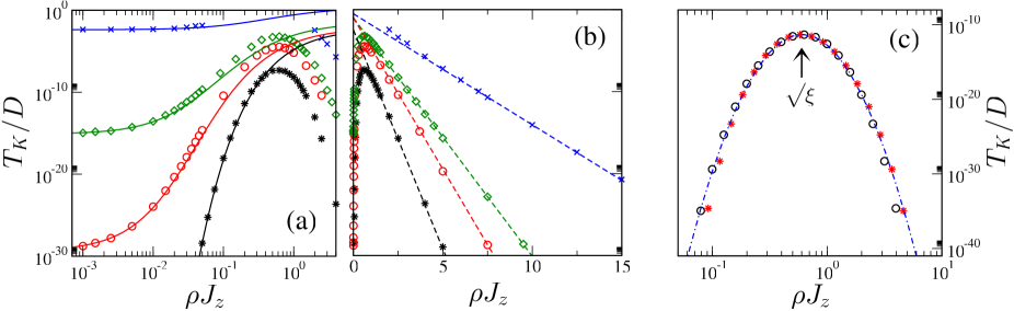
The low behavior, seen most clearly in Fig. 6 (a), can be understood using perturbative scaling. As mentioned in Sec. III, to second-order this yields scaling equations for Eq. (15) that are identical to the regular spin- Kondo model.Béri and Cooper (2012) The equations can be solvedAnderson et al. (1970); Zitko et al. (2008) to give
| (33a) | ||||
| where | ||||
| (33b) | ||||
| with | ||||
| (33c) | ||||
When , there is excellent agreement between exact NRG results for (points) and Eq. (33a) [solid lines, panel (a)]. In each case, we have adjusted the constant to fit the data, implying a weak dependence on of the pre-exponential factor in Eq. (33a), obtained to higher order in perturbative scaling.
When becomes large, the perturbative treatment naturally breaks down. As seen from NRG results in Fig. 6, the Kondo temperature in fact passes through a maximum at , and then decreases rapidly as is further increased. Specifically, we find from NRG for that,
| (34) |
which is plotted for comparison as the dashed lines in Fig. 6 (b). On extrapolating this result, we conclude that that remains finite for any (provided ). (We have also performed a direct survey of the parameter space of the model to substantiate this conclusion further.) As such, while the Kondo temperature is very small for large , there is always overscreening of the ‘impurity’ for antiferromagnetic .
The latter point may not be surprising at first sight. However, in the case of the 4CK model (with the same low-energy NFL fixed point), the ground state is a free local moment state for a sufficiently large, antiferromagnetic .Schiller and De Leo (2008) The argument involves a mapping between the positive and negative sectors, and hence the transition for antiferromagnetic is effectively the same Kosterlitz-Thouless transition well known to arise in the ferromagnetic case.Schiller and De Leo (2008) The absence of such a transition here reflects that, while the fixed points of the two models are the same, the RG flows between these fixed points are very different in the general case of exchange anisotropy (c.f. the discussion of Sec. IV.2).
Further analytical insight is obtained by applying the abelian bosonization technique of Ref. Schiller and De Leo, 2008 to the present problem. We predict a duality in Eq. (15):
| (35) |
with . This result does not hold ubiquitously, however, as the bosonization argument requires that and . To understand the effect of these constraints, it is convenient to define the quantity
| (36) |
from which it follows simply that Eq. (35) holds when
| (37) |
and thus becomes most valid when , i.e. .
Equation (35) is consistent with the absence of a transition for antiferromagnetic since, in contrast to the 4CK model,Schiller and De Leo (2008) the duality does not change the sign of the exchange coupling and therefore does not map the ferromagnetic Kosterlitz-Thouless transition of the model onto the antiferromagnetic side. Instead it simply maps small to large ; in this sense it is similar to the duality inherent to the two-channel Kondo (2CK) model.Kolf and Kroha (2007)
A further consequence of Eq. (35) can be seen by writing Eq. (35) in terms of as
| (38) |
Since the Hamiltonian is invariant to changing the sign of , it follows that
| (39) |
for fixed when Eq. (37) is satisfied. On making the ansatz that has a power series expansion in , one thus obtains
| (40) | ||||
| (41) |
with a constant: this form agrees very well with our NRG results when Eq. (37) is satisfied, albeit with a slightly adjusted . A fit of Eq. (41) to NRG data for is shown in Fig. 6 (c) as the dot-dashed line.
The duality also sheds light on Eq. (34). For , the perturbative scaling result of Eq. (33) is valid, and can be expanded to give
| (42) | ||||
| (43) |
for , such that
| (44) |
with a constant. But since it follows from Eq. (37) that the duality of Eq. (35) holds, and hence
| (45) |
for . This recovers Eq. (34), with asymptotically for small .
V.2 Physical quantities
In addition to the results above, we have calculated the t matrices when . On lowering the channel symmetry we find as expected that . Specifically, the high-frequency logarithmic tails of the t matrices still take the form of Eq. (25) but with different constants. At frequencies , however, we find that the t matrices fall onto the same universal curve as in Fig. 4. This reflects an emergent channel symmetry at the NFL fixed point.Béri and Cooper (2012)
Similar behavior is naturally found when examining the AC conductance. We thus conclude that channel isotropy would not be required in order to observe the non-Fermi-liquid physics of the model described in Sec. IV.
VI Fermi-liquid crossover
Finally, we consider breaking the axial symmetry of Eq. (15) by taking . As shown in Sec. II, this kind of symmetry breaking arises due to non-local Majorana-Majorana, Majorana-lead, or lead-lead couplings in the bare model, Eq. (5). In Sec. III we argued that such perturbations are RG relevant, and drive the system to a strong coupling, Fermi-liquid (FL) ground state. In this section we confirm this explicitly using NRG. Although even tiny perturbations destabilize the NFL fixed point, NFL physics may still be observable at finite energies/temperatures.
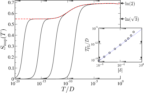
In Fig. 7 we show NRG results for the impurity entropy, with , , and several different values of the symmetry-breaking parameter (solid lines), compared with the case (dashed line). For all finite , the entropy always vanishes, . This is indicative of RG flow to the stable SC Fermi-liquid fixed point. We denote the scale characterizing this flow by , defining it in practice by , suitably halfway between the SC and NFL fixed point values.
CFT allows one to identify relevant operators in the channel sector which have the same symmetry as the perturbation. Owing to axial symmetry, there is one such operator at the NFL fixed point with scaling dimension . This dimension implies that the Fermi-liquid crossover scale has a power-law dependence,
| (46) |
which should apply when acts as a perturbation to the NFL fixed point — i.e., when there is good scale separation . Indeed, this result is confirmed in the inset to Fig. 7, by comparison of NRG results (points) to Eq. (46) (dotted line).
Although any nonzero destabilizes the NFL fixed point, signatures of non-Fermi-liquid physics should still be observable in an intermediate temperature ‘window’, provided the strength of perturbations is small (as might be expected physically, see Sec. II). As seen from Fig. 7, when there is good scale separation , thermodynamics at higher temperatures are essentially indistinguishable from the case (where the NFL fixed point is stable down to ). The topological Kondo effect could thus be identifiable in this regime, even when symmetry-breaking perturbations act. Indeed, at lower temperatures, the subsequent Fermi-liquid crossover is wholly characteristic of flow from the unstable NFL fixed point, and exhibits universal scaling in terms of . Thus, flow away from the NFL fixed point due to symmetry-breaking perturbations could also be used to identify the topological Kondo effect.
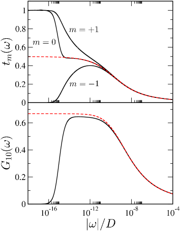
Dynamics of the model when are of particular interest. In the top panel of Fig. 8, we show the three t matrices , when and , with . The corresponding t matrices for are shown as the dashed line (these are identical by symmetry in this isotropic limit). Here, is sufficiently small that the NFL fixed point strongly affects the RG flow and resulting t matrix lineshapes. When there is good scale separation, we find for the asymptotic behavior of
| (47) |
The behavior of is consistent with first-order corrections from the relevant operator mentioned above, while the deviations of and appear to arise at the second-order level. Interestingly, in the basis of Eq. (12), the t matrix in channel is essentially indistinguishable from the case for energies , and we find .
At lower energies , the perturbation grows under RG and becomes large, causing deviation from this behavior. Near the Fermi-liquid fixed point we instead find for that
| (48) |
This is characteristic of standard strong coupling Kondo physics in leads and , with lead decoupling asymptotically. The roles of are reversed when , since the Kondo effect then takes place with leads and . The t matrices thus indicate directly which channels are participating in the Kondo effect at the SC fixed point, and support the physical picture discussed in Sec. III.
The low-energy crossover to the SC fixed point (and the associated ‘window’ of non-Fermi-liquid behavior) is also seen in the AC conductance, shown in the bottom panel of Fig. 8 for the same parameters as the t matrices discussed above. We find asymptotically that
| (49) |
Interestingly, as here, despite the fact that channels and form a Kondo singlet with the central impurity spin for (typically the Kondo effect results in a zero-bias enhancement of conductance). The vanishing conductance (between channels and ), is in fact due to the decoupling of the third channel, , at the strong coupling fixed point. This can be understood by the following physical argument: an electron tunneling from lead to requires (by conservation of total ) to flip the impurity spin from to . Further electronic transport is now blocked, since the impurity mediates the current between all channels, and is already in the configuration. Only when lead is coupled in can a finite conductance result: the impurity configuration can be restored (thus ‘resetting’ the system) by a tunneling process from to . The Fermi-liquid ground state of the model (arising from any inter-Majorana coupling) thus inevitably results in vanishing conductance; although of course signatures of criticality and non-Fermi-liquid physics may appear at finite temperatures. Naturally, similar results are obtained for .
One might ask how the results above change when the non-local perturbations are larger, e.g. of order or more. In this case, the NFL fixed point (characterized by fractional power-law behaviour) seen on decreasing or will of course not be directly observable. The system will flow away to the SC fixed point on the energy scale of the perturbations, and hence the conductance will drop to zero before the power-law behavior is reached. But the key signature of the topological Kondo effect itself—the approach to the NFL fixed point, characterized by the low frequency/temperature conductance peak—could still be observable for such large perturbations. This is aided by the fact that the approach to the NFL fixed point is very slow (compared to that of the conventional Kondo effect, see Fig. 5), taking place over a very wide energy range that starts several orders of magnitude above .
VII Conclusion
We have analyzed in detail the physics of the minimal topological Kondo setup of Fig. 1, starting from its most symmetric limit of a spin- Kondo impurity coupled isotropically to spin conduction electrons, gradually breaking its symmetries, and then including the small nonlocal couplings not considered in Ref. Béri and Cooper, 2012. Using the NRG, we have obtained accurate results for the model, including directly-measurable quantities such as the differential conductance, on energy scales ranging over many orders of magnitude.
The spin-isotropic limit of the model displays a universal crossover from local moment to non Fermi liquid fixed points, the latter being characterised by non-trivial power-law corrections to the low-temperature/frequency physics. Since the spin sector of the present model is the same as that of the four-channel Kondo model, many of the full crossover curves we have calculated here tend toward known asymptotes for the latter model. On the other hand, quantities depending on the details of the charge and orbital sectors, such as the scattering t-matrix and differential conductance, show quite distinct physics.
Focussing on the differential conductance, we showed that this has characteristic logarithmic tails at high energies, which cross over to power-law behavior with exponent at low energies,Béri and Cooper (2012) as shown in Fig. 5. The NRG results show that the power law scaling sets in for energy scales and the logarithmic tails require . Depending on the value of the Kondo temperature, observing either or both of these asymptotes might be difficult in experiment. The universal scaling curve (in terms of ) obtained here by NRG, with its far broader domain than those of the asymptotes, is therefore indispensable for full quantitative comparisons to experiments.
We find, as predicted in Ref. Béri and Cooper, 2012, that the physics of the model is robust to exchange anisotropy (which would arise physically due to differences between the tunnel couplings in the device). Furthermore, we found that the small and large regimes are related by a duality when is sufficiently weak. This duality is reminiscent of that seen in the two-channel Kondo model,Kolf and Kroha (2007) and enables analytical weak-coupling perturbative scaling results to be carried over to the large- regime.
Including non-local coupling between the Majoranas breaks the effective time-reversal symmetry of the model, causing a crossover ultimately to the strong coupling, Fermi liquid fixed point. As long as the perturbations are sufficiently weak that the energy scale of the Fermi liquid crossover is , data collapse onto the scaling curve of the unperturbed problem for a wide range of energies , see Fig. 8. In this case, the NFL to Fermi liquid crossover itself also has its own universal scaling curve in terms of , providing another signature of the NFL physics.
For larger perturbations, of order and above, the NFL fixed point will not be approached so closely. But even in this situation, part of the slow crossover from the local moment to NFL fixed point could potentially be observed in experiment, thus providing a signature of the topological Kondo effect—and hence the existence of Majorana fermions—in a real device.
Acknowledgements.
This research was supported by EPSRC grants EP/I032487/1 (AKM,DEL) and EP/J017639/1 (NRC), the MC IEF and the Royal Society (BB).Appendix A Correlation functions for scattering t-matrix
For a system described by the general Hamiltonian
| (50) |
in which describes an interacting subsystem coupled to the orbitals, and is a ‘flavor’ index, standard equations of motion techniques lead to the result
| (51) |
where and denotes the Fourier transform to the domain of the retarded correlation function . The term in square brackets in Eq. (51) describes describes scattering due to and will be related to the on-shell t matrix below.
The Hamiltonian Eq. (15) is of precisely the form of Eq. (51), with given by the terms involving the ‘impurity’ spin operators. From Eq. (13) we obtain , and use the relation to obtain
| (52) |
with
| (53a) | ||||
| (53b) | ||||
| (53c) | ||||
Defining as the quantity in square brackets in Eq. (51), it follows from Eq. (53) that the on-shell t-matrix is given by
| (54) | ||||
| (55) |
Of primary interest is the spectral function of , which we define as the dimensionless quantity
| (56) |
Appendix B Kubo formula for conductance
The conductance tensor of the model can be calculated for both the original basis of Eq. (9) and the transformed basis of Eq. (15). For the most part, the derivations are essentially identical, since only number operators of the lead electrons enter (rather than the interaction part of the Hamiltonian which is strongly basis-dependent). We therefore begin by outlining the part of the derivation common to both bases.
Our starting point is the standard result from Appendix B of Hewson Hewson (1997). To leading order in the perturbation, the change in expectation value of an operator from its equilibrium value, due to an adiabatically-switched-on perturbation (with , is
| (57) |
where , the density matrices in the presence [absence] of the perturbation are [], and
| (58) |
with the Hamiltonian of the equilibrium system. Taking the perturbation to be
| (59) |
(with the magnitude of the electron charge and the frequency of the AC bias voltage), the current into lead ,
| (60) |
is given by
| (61) |
Here, we use to denote the total number operator of lead , either in the original basis of Eq. (9), or the transformed basis of Eq. (15).
The change of variable leads to
| (62) |
i.e.
| (63) |
with
| (64) |
as defined by Izumida et al.Izumida et al. (1997) Following the manipulations therein, we obtain (for )
| (65) | ||||
| (66) |
where
| (67) | ||||
| (68) |
In the limit, we obtain the steady-state (-independent) DC conductance
| (69) |
At finite , for specificity we focus henceforth on the value of the conductance,
| (70) |
which thus probes the frequency dependence of the same spectral function , and satisfies
| (71) |
By Lehmann-resolving (see ref. Izumida et al., 1997), one obtains
| (72) |
and hence, from Eq. (70),
| (73) |
To check this sign, one can examine the DC limit. Using Eq. (59) with , a positive bias applied to lead will raise its chemical potential, such that the current into lead obtained from Eq. (60) [and hence the conductance from Eq. (65)] should indeed be negative.
B.1 Symmetries of the conductance
For specificity we focus on a particular off-diagonal element, of the conductance tensor. As explained below, in the axial-symmetric limit of the model it has the convenient properties of a) being the same in both bases, and b) being proportional also to the diagonal element .
We denote by and the number operators for the leads in the physical basis of Eq. (9) and the transformed basis of Eq. (15), respectively. It is straightforward to show that
| (74a) | ||||
| (74b) | ||||
It thus follows from eqns. (67) and (70) that
| (75a) | ||||
| (75b) | ||||
where and denote the conductance in the physical and transformed bases, respectively.
Two sets of further results hold in each basis: axial symmetry implies that
| (76a) | ||||
| (76b) | ||||
while current conservation means that
| (77a) | ||||
| (77b) | ||||
Combining eqns. (75), (76) and (77), we obtain
| (78) |
[Here, the minus signs reflect that, for a particular bias applied to lead , the currents flowing from the ‘impurity’ to leads and will be in opposite directions, and the inequality is obtained from Eq. (73).] The single quantity thus provides a useful handle on the conductance of the model in both bases.
In the fully isotropic limit of the model, Eq. (78) can of course be extended by symmetry: the full tensors and are identical, with
| (79) |
for all . In this case, therefore, the single quantity represents all elements of both conductance tensors.
B.2 Calculation via NRG
To calculate by NRG, one needs the time-derivatives of the lead operators in Eq. (67). Using
| (80) |
one obtains with
| (81) | ||||
| (82) | ||||
| (83) |
(the latter equality reflecting the current conservation in the system).
Matrix elements of these operators can be calculated, and then used to obtain the correlation function in Eq. (67) by the FDM-NRG method.Weichselbaum and von Delft (2007) Owing to the discretization inherent in the NRG approach, one obtains a discrete set of delta functions which lead to a similarly discrete representation of when Eq. (70) is used. We then broaden the poles of using the standard method of Ref. Weichselbaum and von Delft, 2007.
References
- Read and Green (2000) N. Read and D. Green, Phys. Rev. B 61, 10267 (2000).
- Kitaev (2001) A. Y. Kitaev, Physics-Uspekhi 44, 131 (2001).
- Fu and Kane (2008) L. Fu and C. Kane, Phys. Rev. Lett. 100, 96407 (2008).
- Sau et al. (2010a) J. Sau, R. Lutchyn, S. Tewari, and S. Das Sarma, Phys. Rev. Lett. 104, 40502 (2010a).
- Alicea (2010) J. Alicea, Phys. Rev. B 81, 125318 (2010).
- Oreg et al. (2010) Y. Oreg, G. Refael, and F. von Oppen, Phys. Rev. Lett. 105, 177002 (2010).
- Alicea (2012) J. Alicea, Rep. Prog. Phys. 75, 076501 (2012).
- Beenakker (2013) C. W. J. Beenakker, Annu. Rev. Con. Mat. Phys. 4, 113 (2013).
- Nayak et al. (2008) C. Nayak, S. Simon, A. Stern, M. Freedman, and S. Sarma, Rev. Mod. Phys. 80, 1083 (2008).
- Mourik et al. (2012) V. Mourik, K. Zuo, S. M. Frolov, S. R. Plissard, E. P. A. M. Bakkers, and L. P. Kouwenhoven, Science 336, 1003 (2012).
- Das et al. (2012) A. Das, Y. Ronen, Y. Most, Y. Oreg, M. Heiblum, and H. Shtrikman, Nat. Phys. 8, 887 (2012).
- Deng et al. (2012) M. T. Deng, C. L. Yu, G. Y. Huang, M. Larsson, P. Caroff, and H. Q. Xu, Nano Letters 12, 6414 (2012).
- Rokhinson et al. (2012) L. P. Rokhinson, X. Liu, and J. K. Furdyna, Nat. Phys. 8, 795 (2012).
- Williams et al. (2012) J. R. Williams, A. J. Bestwick, P. Gallagher, S. S. Hong, Y. Cui, A. S. Bleich, J. G. Analytis, I. R. Fisher, and D. Goldhaber-Gordon, Phys. Rev. Lett. 109, 056803 (2012).
- Knez et al. (2012) I. Knez, R.-R. Du, and G. Sullivan, Phys. Rev. Lett. 109, 186603 (2012).
- Law et al. (2009) K. T. Law, P. A. Lee, and T. K. Ng, Phys. Rev. Lett. 103, 237001 (2009).
- Wimmer et al. (2011) M. Wimmer, A. R. Akhmerov, J. P. Dahlhaus, and C. W. J. Beenakker, New J. Phys. 13, 053016 (2011).
- Sau et al. (2010b) J. D. Sau, S. Tewari, R. M. Lutchyn, T. D. Stanescu, and S. Das Sarma, Phys. Rev. B 82, 214509 (2010b).
- Pientka et al. (2012) F. Pientka, G. Kells, A. Romito, P. W. Brouwer, and F. von Oppen, Phys. Rev. Lett. 109, 227006 (2012).
- Bagrets and Altland (2012) D. Bagrets and A. Altland, Phys. Rev. Lett. 109, 227005 (2012).
- Pikulin et al. (2012) D. Pikulin, J. Dahlhaus, M. Wimmer, H. Schomerus, and C. Beenakker, New J. Phys. 14, 125011 (2012).
- Liu et al. (2012) J. Liu, A. C. Potter, K. Law, and P. A. Lee, Phys. Rev. Lett. 109, 267002 (2012).
- Kells et al. (2012) G. Kells, D. Meidan, and P. W. Brouwer, Phys. Rev. B 86, 100503 (2012).
- Hassler et al. (2010) F. Hassler, A. R. Akhmerov, C. Y. Hou, and C. W. Beenakker, New J. Phys. 12, 125002 (2010).
- Sau et al. (2010c) J. D. Sau, S. Tewari, and S. Das Sarma, Phys. Rev. A 82, 052322 (2010c).
- Alicea et al. (2011) J. Alicea, Y. Oreg, G. Refael, F. Von Oppen, and M. P. A. Fisher, Nat. Phys. 7, 412 (2011).
- van Heck et al. (2012) B. van Heck, A. Akhmerov, F. Hassler, M. Burrello, and C. Beenakker, New J. Phys. 14, 035019 (2012).
- Hyart et al. (2013) T. Hyart, B. van Heck, I. C. Fulga, M. Burrello, A. R. Akhmerov, and C. W. J. Beenakker, Phys. Rev. B 88, 035121 (2013).
- Béri and Cooper (2012) B. Béri and N. R. Cooper, Phys. Rev. Lett. 109, 156803 (2012).
- Fu (2010) L. Fu, Phys. Rev. Lett. 104, 056402 (2010).
- Tsvelik (2013) A. M. Tsvelik, Phys. Rev. Lett. 110, 147202 (2013).
- Crampe and Trombettoni (2013) N. Crampe and A. Trombettoni, Nucl. Phys. B (2013).
- Béri (2013) B. Béri, Phys. Rev. Lett. 110, 216803 (2013).
- Altland and Egger (2013) A. Altland and R. Egger, Phys. Rev. Lett. 110, 196401 (2013).
- (35) A. Zazunov, A. Altland, and R. Egger, “Transport properties of the coulomb-majorana junction,” arXiv:1307.0210.
- Fabrizio and Gogolin (1994) M. Fabrizio and A. O. Gogolin, Phys. Rev. B. 50, 17732 (1994).
- Fabrizio and Zarand (1996) M. Fabrizio and G. Zarand, Phys. Rev. B. 54, 10008 (1996).
- Nozières and Blandin (1980) P. Nozières and A. Blandin, J. Phys. (Paris) 41, 193 (1980).
- Bulla et al. (2008) R. Bulla, T. A. Costi, and T. Pruschke, Rev. Mod. Phys. 80, 395 (2008).
- Andrei and Destri (1984) N. Andrei and C. Destri, Phys. Rev. Lett. 52, 364 (1984).
- Tsvelik (1985) A. M. Tsvelik, J. Phys. C 18, 159 (1985).
- Schiller and De Leo (2008) A. Schiller and L. De Leo, Phys. Rev. B. 77, 075114 (2008).
- Hewson (1997) A. C. Hewson, The Kondo Problem to Heavy Fermions (Cambridge University Press, Cambridge, 1997).
- Note (1) Moving away from the middle of the Coulomb blockade valley would generate non-universal (but RG-marginal) potential scattering terms in .Béri and Cooper (2012) We have checked numerically that that the non-Fermi-liquid fixed point discussed in Sec. III is robust to their inclusion; their effect on physical properties such as the finite-/finite- differential conductance is left for future work.
- Note (2) If one takes , the coupling constants in Eq. (15) are simply related to those of Eq. (9) by , and . Non-local couplings generate the term and unequal , and then the relationship between the two sets of coupling constants becomes more complicated.
- Anders and Schiller (2005) F. B. Anders and A. Schiller, Phys. Rev. Lett. 95, 196801 (2005).
- Weichselbaum and von Delft (2007) A. Weichselbaum and J. von Delft, Phys. Rev. Lett. 99 (2007).
- Peters et al. (2006) R. Peters, T. Pruschke, and F. B. Anders, Phys. Rev. B. 74 (2006).
- Oliveira and Oliveira (1994) W. C. Oliveira and L. N. Oliveira, Phys. Rev. B. 49, 11986 (1994).
- Anderson (1970) P. W. Anderson, J. Phys. C 3, 2346 (1970).
- Dickens and Logan (2001) N. L. Dickens and D. E. Logan, J. Phys.: Condens. Matt. 13, 4505 (2001).
- Tsvelick and Wiegmann (1983) A. Tsvelick and P. Wiegmann, Adv. Phys. 32, 453 (1983).
- Andrei et al. (1983) N. Andrei, K. Furuya, and J. H. Lowenstein, Rev. Mod. Phys. 55, 331 (1983).
- Note (3) We noteKrishnamurthy et al. (1980) that the same perturbation connects degenerate charge states of the ‘free orbital’ fixed point in the regular Anderson impurity model.
- Affleck (1990) I. Affleck, Nucl. Phys. B 336, 517 (1990).
- Affleck and Ludwig (1991a) I. Affleck and A. Ludwig, Nucl. Phys. B 352, 849 (1991a).
- Affleck and Ludwig (1991b) I. Affleck and A. Ludwig, Nucl. Phys. B 360, 641 (1991b).
- Affleck and Ludwig (1993) I. Affleck and A. W. W. Ludwig, Phys. Rev. B 48, 7297 (1993).
- Sengupta and Kim (1996) A. M. Sengupta and Y. B. Kim, Phys. Rev. B. 54, 14918 (1996).
- (60) A. K. Mitchell, M. R. Galpin, S. Wilson-Fletcher, D. E. Logan, and R. Bulla, arXiv:1308.1903.
- Jones et al. (1988) B. A. Jones, C. M. Varma, and J. W. Wilkins, Phys. Rev. Lett. 61, 125 (1988).
- Jones (1991) B. A. Jones, Physica B 171, 53 (1991).
- Affleck and Ludwig (1992) I. Affleck and A. W. W. Ludwig, Phys. Rev. Lett. 68, 1046 (1992).
- Affleck et al. (1995) I. Affleck, A. W. W. Ludwig, and B. A. Jones, Phys. Rev. B. 52, 9528 (1995).
- Mitchell et al. (2012) A. K. Mitchell, E. Sela, and D. E. Logan, Phys. Rev. Lett. 108, 086405 (2012).
- Zubarev (1960) D. N. Zubarev, Sov. Phys. Usp. 3, 320 (1960).
- Note (4) For the 1CK model, ; and we define via .
- Izumida et al. (1997) W. Izumida, O. Sakai, and Y. Shimizu, J. Phys. Soc. Japan 66, 717 (1997).
- Note (5) NRG recovers the exact value to within a few percent (although numerical errors can in principle be systematically reduced). In our analysis of the low-frequency power-law behavior of , we therefore treated as a fitting parameter. A fit to the form extends to the lowest frequencies, compared with other simple rational powers.
- Note (6) We use the standard broadening schemeBulla et al. (2008); Weichselbaum and von Delft (2007); *Peters2006 for calculating NRG spectra on temperature scales , which has been shownMitchell and Sela (2012) to reproduce accurately the full frequency and temperature dependence of dynamical quantities for other quantum impurity problems where exact results are known.
- Anderson et al. (1970) P. W. Anderson, G. Yuval, and D. R. Hamann, Phys. Rev. B. 1, 4464 (1970).
- Zitko et al. (2008) R. Zitko, R. Peters, and T. Pruschke, Phys. Rev. B. 78 (2008).
- Kolf and Kroha (2007) C. Kolf and J. Kroha, Phys. Rev. B 75, 045129 (2007).
- Krishnamurthy et al. (1980) H. R. Krishnamurthy, J. W. Wilkins, and K. G. Wilson, Phys. Rev. B. 21, 1003 (1980).
- Mitchell and Sela (2012) A. K. Mitchell and E. Sela, Phys. Rev. B 85, 235127 (2012).