A Radio Determination of the Time of the New Moon

Abstract

The detection of the New Moon at sunset is of importance to communities based on the lunar calendar. This is traditionally undertaken with visual observations. We propose a radio method which allows a higher visibility of the Moon relative to the Sun and consequently gives us the ability to detect the Moon much closer to the Sun than is the case of visual observation. We first compare the relative brightness of the Moon and Sun over a range of possible frequencies and find the range 5–100 GHz to be suitable. The next consideration is the atmospheric absorption/emission due to water vapour and oxygen as a function of frequency. This is particularly important since the relevant observations are near the horizon. We show that a frequency of $\sim 10$ GHz is optimal for this programme. We have designed and constructed a telescope with a FWHM resolution of 0${}^{\circ}{}\!\!$.6 and low sidelobes to demonstrate the potential of this approach. At the time of the 21 May 2012 New Moon the Sun/Moon brightness temperature ratio was $72.7\pm 2.2$ in agreement with predictions from the literature when combined with the observed sunspot numbers for the day. The Moon would have been readily detectable at $\sim 2^{\circ}$ from the Sun. Our observations at 16 hr 36 min UT indicated that the Moon would have been at closest approach to the Sun 16 hr 25 min earlier; this was the annular solar eclipse of 00 hr 00 min UT on 21 May 2012.

1 Introduction

Throughout history, dating back to Babylonian times, the first appearance of the New Moon has been used to determine the calendar. Hindu, Hebrew and Muslim calendars are based on the visual sighting of the first cresent Moon after conjunction with the Sun at the beginning of each month (Bruin, 1977). Today, most lunar calendars are based on calculation with a mean lunar synodic period of 29.35 solar days. However, many observe a religious lunar calendar using actual visual observations of the setting crescent Moon.

The visual sighting by the naked eye of the first crescent after New Moon (Sun-Moon conjunction) depends on the angular distance between the Moon and the Sun at sunset. Typically, twenty four hours after conjunction, the Moon has moved $\sim 12$^∘ in Right Ascention (RA) from the Sun and the Moon illumination will be about 1 per cent. Under these conditions, the Moon will set approximately 40 min after sunset (depending on the observer’s geographical latitude) when the sky luminosity has decreased. Provided the sky is sufficiently clear, these factors (lower sky luminosity and and increased illumination) combine to make the crescent Moon visible for few minutes with the naked eye before it sets. If sunset occurs much less than twenty four hours after conjunction, the angular separation between the Moon and the Sun is not sufficient for the sighting to be performed.

We propose a radio method for the determination of the time of New Moon. This method is independent of the weather and can be used to establish the exact time of the New Moon with much higher accuracy than the traditional visual method. At optical frequencies, the full Moon is a factor of 4$\times$10⁵ fainter than the Sun; in the radio range, this factor is reduced to approximately 100–500. The challenge is to detect the weaker signal from the Moon in the presence of the much brighter Sun and also to account for the atmospheric emission and absorption at low elevation. Both the Sun and the Moon have variable brightness. The Sun changes with the 27-day solar rotation and the 11.3-year sunspot cycle. The Moon varies with the lunar 29.3-day cycle. In addition the Sun shows strong variation with frequency; the Moon is less variable. The choice of an optimal radio frequency is critical for this project.

The paper is set out as follows. Section 2 describes the frequency dependence of the various components of solar emission. Section 3 gives the frequency dependence of the lunar emission including the variation with lunar phase. The atmospheric opacity of H₂O and O₂ are discussed in Section 4. This is required because the observations are made at low elevation where absorption and emission effects are significant. Section 5 describes a working system at 10 GHz. It includes observations 16 hr after New Moon on 21 May 2012, demonstrating the potential of such a system for direct observation of the New Moon. Conclusions are given in Section 6.

2 The radio properties of the Sun

The radio emission of the Sun comes from the corona, the chromosphere and the photosphere in various proportions depending on the frequency. The $10^{6}$ K corona dominates the emission at frequencies below $\sim 1$ GHz where its free-free emission becomes optically thick. At 50 GHz and above the photosphere (electron temperature, $T_{e}=6000$ K) is the major contributor. At 5 to 30 GHz the chromosphere ($T_{e}=10000$ K) is also a significant component and is the source of the radio variability.

We now consider the relationship between the optical and radio emission from the Sun in its quiet and active modes.

2.1 The brightness temperature of the quiet Sun

The brightness temperature, $T_{b}$, of the Sun at a given frequency can be expressed as the value which will give the observed flux density when averaged over the optical diameter. We confine our study to frequencies above 1 GHz where $T_{b}<10^{5}$ K in order that the Sun is considerably less than 1000 times the Moon emission (see Section 3). The quiet Sun emission is defined as that observed/estimated for zero sunspots. The quiet Sun $T_{b}$ values at times of sunspot maximum and minimum are given in Table 1 for representative frequencies of interest for this project. These values are derived from the multiplicative terms given by Cox (2000) and cross-checked with data given by Kundu (1965) and by Covington & Medd (1954).

Table 1 shows that for frequencies less than 10 GHz the quiet Sun $T_{b}$ increases approximately as wavelength squared, as expected for an optically thin solar corona. At 10–20 GHz the emission is dominated by the optically thick chromosphere; at 50 GHz and above we approach the optically thick photosphere with $T_{b}=6000$ K. The ratio of the quiet Sun $T_{b}$ at sunspot maximum to minimum is highest ($\sim 1.5$) at frequencies dominated by coronal emission. At 10 GHz the ratio is 1.32.

		Quiet Sun $T_{b}$		$T_{b}$ ratio	Increase of
$\lambda$	$\nu$	SS min	SS max		SS min $T_{b}$
(cm)	(GHz)	(1000 K)	(1000 K)		(per cent)
(1)	(2)	(3)	(4)	(5)	(6)
30	1.0	132	218	1.65	110
15	2.0	56	85	1.51	126
6.0	5.0	21.4	31.6	1.48	68
3.0	10	12.6	16.6	1.32	17
1.5	20	9.5	11.0	1.16	2
0.6	50	6.8	7.4	1.10	0
0.3	100	6.3	6.5	1.03	0

Table 1: The radio brightness temperature of the Sun in the frequency range 1–100 GHz. The sunspot maximum (SS max) and minimum (SS min) values for the steady component (i.e. at $R=0$) are given in columns 3 and 4. Column 5 gives the brightness temperature ratio between sunspot maximum and minimum. Column 6 gives the component correlated with sunspot number for $R=100$. $R$ is defined as $10N_{g}+N_{s}$ where $N_{g}$ is the number of sunspot groups and $N_{s}$ is the number of individual sunspots.

2.2 Variation of emission over the sunspot cycle

The 11.3-year sunspot cycle can be seen at all frequencies from radio to X-rays. In the frequency range of 1–100 GHz considered here the emission is closely correlated with the sunspot activity measured either as the sunspot area or the sunspot number. It has become conventional to use the sunspot number $R$, defined as $R=10N_{g}+N_{s}$ where $N_{g}$ is the number of sunspot groups and $N_{s}$ is the number of individual spots (Cox, 2000).

Fig. 1 shows the monthly averaged values of $R$ from 1980 to the present. Predicted values for the remainder of the current sunspot maximum are shown as full lines to represent the mean value of $R$ and the upper and lower bounds. The sunspot data are from the Solar Influences Data Analysis Center . It is seen that the level of activity varies from cycle to cycle. For example the most recent cycle lasted for an unusually long period and the present maximum promises to be weaker than average.

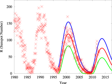
Figure 1: Monthly sunspot numbers ($R$) from 1980 to the present. The sunspot number data are from the Solar Influences Data Analysis Center.¹ The solar cycle model for the 23^rd cycle (1998–2009) and the prediction for the 24^th cycle (2009–2020) in red line is based on Hathaway et al. (1994). The blue line gives the prediction for 95 per cent of the observations being below this level and the green line is for 95 per cent above.

A shorter period of variability arises from the 27-day rotation period of the Sun as defined by the active areas with their associated sunspots. These active areas can last from a few days to a few months as the sunspots are born and decay. The larger sunspot groups last for several rotation periods as can be seen in Fig. 2, which shows the daily values of $R$ for 2001 (near sunspot maximum) and for 2011 (near the most recent sunspot minimum).

Figure 2: Daily sunspot numbers, $R$, covering a year near the previous sunspot maximum (2001) in blue compared with a year at the rise from the recent sunspot minimum (2011) plotted in red. The 27-day period of the longer-lasting groups can be seen in both years. Note the ordinate is sunspot number $R$. Data are taken from the published values on the Solar Influences Data Analysis Center website.¹

The close correlation between the 2.8 GHz radio emission (Covington, 1974) and the monthly values of sunspot number is illustrated in Fig. 3 which covers the sunspot cycle running from 1954 to 1964. The quiet Sun at sunspot minimum is 66 flux units and rises to $\sim 120$ flux units at sunspot maximum. The variable $R$-correlated emission more than doubles this level. This result can be checked against the predictions of Table 1. The peak sunspot number is $R=250$ which would add another 120 flux units at sunspot maximum giving a total of $\sim 240$ flux units in agreement with Fig. 3. Clearly there is significant variation in the radio emission over the solar cycle that needs to be taken into account in the present study.

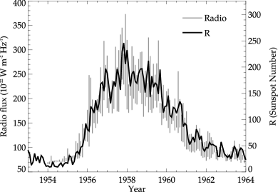
Figure 3: A comparison of the 2.8 GHz flux density in units of $10^{-22}$ W m^-2 Hz^-1 with the sunspot number, $R$, for the period of one sunspot cycle from 1954 to 1964. The range of flux density in each month is plotted. Note that the radio emission for R$\sim$0 (sunspot minimum) corresponds to $\sim 60$ flux units due to the steady chromosphere emission The radio data are from Covington (1974); the sunspot data are from the Solar Influences Data Analysis Center¹.

2.3 Variability over timescales $<<1$ day

The main variability on timescales $<<1$ day arises from the radio bursts associated with solar flares. At 2.8 GHz, for example, typical bursts last 2 min to 50 min (Covington & Medd, 1954). These occur in various forms, with the two most common being a single burst and a single burst with a following enhancement. Peak flux values are 10–20 per cent of the quiet Sun. Analysis of the flare data of Dodson et al. (1954) indicated that 57 per cent of the brightest flares (types 2 and 3) had associated radio bursts. The frequency of occurrence of the stronger bursts was one every few days and consequently will have little effect on the present programme, which tracks the Sun/Moon for periods of several hours at least.

2.4 The diameter of the quiet and active Sun as a function of frequency

This is a small effect at frequencies where the chromospheric and photospheric emission dominates, being the optical value. The solar optical diameter at the mean Sun-Earth distance is 32.0 arcmin. The diameter changes by $\pm 1.67$ per cent beween aphelion and perihelion. Consequently at 10 GHz and above the diameter can be taken as the optical value but with some limb-darkening in the polar direction.

At 1.4 GHz the diameter of the quiet Sun is 1.1 times the optical value (Christiansen & Warburton, 1955). At the much lower frequency of 200 MHz the effective diameter is $1.5\times 1.2$ times the optical value with the greater extent in the equatorial direction (Kundu, 1965).

The active Sun at frequencies above 1 GHz is produced by heated regions lying above sunspot and plage areas (Christiansen et al., 1957). These can extend up to 5 arcmin (0.2 solar diameter) above the quiet Sun level.

3 The radio properties of the Moon

In this section we consider the properties of the Moon as a function of frequency. In the present case we are concerned with the detection of the Moon in the presence of the much stronger Sun where we use an observing beam which encompasses the whole Moon disk. The integrated properties are the total flux density or the corresponding brightness temperature averaged over the the lunar disc. There is a significant phase effect, which varies significantly in amplitude and phase over the radio range.

$\lambda$	$\nu$	$T_{0}$	$T_{1}$	Phase from
		(average)	(1st harmonic)	New Moon
(cm)	(GHz)	(K)	(K)	(∘)
0.1	300	203	101	5
0.2	150	208	80	14
0.3	100	210	72	17
0.4	75	211	62	24
0.8	37	214	38	32
1.6	19	215	29	35
3.2	9.4	217	14	40
9.6	3.1	221	4	42
20	1.5	224	0.0	–
30	1.0	226	0.0	–

Table 2: Brightness temperature of the Moon at selected frequencies; the data are from Krotikov & Pelyushenko (1987). Listed are the mean brightness temperatures over a lunation, $T_{0}$, the amplitude of the 29.3-day first harmonic, $T_{1}$, and the phase shift of this harmonic as measured from the time of New Moon, $\xi$.

3.1 The mean brightness temperature at radio frequencies

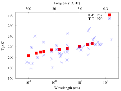
Figure 4: The mean brightness temperature $T_{0}$ of the Moon as a function of wavelength. The blue circle data points are from Troitskii & Tikhonova (1970). The red squares are the model of Krotikov & Pelyushenko (1987).

A substantial body of observations of the Moon is available which covers a wide frequency range (Hagfors, 1970). In recent times, the Moon has been widely used as a calibrator for radio brightness (Linsky, 1973; Harrison et al., 2000; Poppi et al., 2002; QUIET Collaboration et al., 2012) and lunar emission data have been used to complement information from dust samples returned from the Apollo landings (Heiken et al., 1991) and from the lunar orbiter CE-1 (Zheng et al., 2009). It is found that there is a variation of brightness across the surface dependent upon the local properties of the regolith (Zhang et al., 2012). Theoretical modelling of the the lunar material indicates that the depth from which the emission comes is $\approx 10$ times the wavelength (Linsky, 1973).

The mean brightness temperatures of the Moon $T_{0}$ taken from the literature (Troitskii & Tikhonova, 1970) are shown in Fig. 4 for the wavelength range 0.1 to 100 cm. Also plotted in red squares is a more recent assessment of the data (Krotikov & Pelyushenko, 1987). The paper by Zhang et al. (2012) summarizes modern observations which show a mean brightness at 1.4 GHz ($\lambda\approx$21 cm) of $233\pm 2$ K. This indicates that the mean temperature at a depth of $\approx 2$ m is 20 to 30 K higher than in the thin surface layer responsible for the emission at sub-millimetre wavelengths (Fig. 4). Typical values of the mean brightness temperature of the Moon are given in Table 2 for the frequency range of concern here.

3.2 The brightness temperature variation with lunar phase

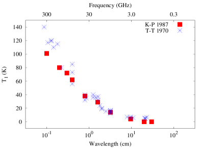
Figure 5: The amplitude of the first harmonic surface brightness $T_{1}$ of the Moon. The description is as for Fig. 4.

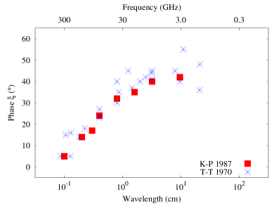
Figure 6: The phase offset of the first harmonic mean surface brightness measured relative to the time of New Moon. The description is as for Fig. 4.

The brightness temperature of the Moon varies in frequency and time during the 29.3-day lunar phase. At any frequency this can be expressed as a harmonic series. Higher harmonics are required at FIR and millimetre wavelengths. The mean temperature $T_{0}$ and the first harmonic, $T_{1}$, are adequate to describe the temperature variation at the lower frequencies required for the present project. We use:

$${T}(\nu)={T}_{0}(\nu)+{T}_{1}(\nu)\cos{}(\omega t-\xi(\nu))~{},$$ (1)

where $\omega$ is the angular frequency of the lunar cycle (12${}^{\circ}\!$.26 per day) and $\xi(\nu)$ is the phase relative to the time of New Moon.

The amplitude of the first harmonic phase variation is shown in Fig. 5. The values of $T_{1}$ at typical frequencies of interest for this project are given in Table 2. The source of the data is as for Fig. 4 with a best-fit model (Krotikov & Pelyushenko, 1987) indicated by red squares. It is seen that the variation is greatest ($\approx 100$ K) at high frequencies where the emission comes from a thin surface layer. At frequencies less than $\approx 3$ GHz ($\lambda\geq 10$ cm), the emission probes a depth of $\approx 1$ m, the variation of $T_{1}$ is less than 4 K.

The phase offset $\xi$ of the first harmonic $T_{1}$ as measured from the time of New Moon is shown in Fig. 6 for the same data set as used in Fig. 4 and 5. Table 2 gives values of $\xi$ at representative frequencies. The phase offset is small ($<5$^∘) at frequencies $\geq 300$ GHz ($\lambda<0.1$ cm) and rises to $\approx 40$^∘ at frequencies $\leq 10$ GHz ($\lambda>3$ cm). It is seen that the phase effect is significant at the frequencies of concern for the present study.

4 The atmospheric emission as related to the project

The emission from the atmosphere is an important consideration when following the Sun and the Moon to the western horizon at sunset. The main components that contribute to atmospheric emission at radio and millimetre wavelengths are molecular oxygen (O₂) and water vapour (H₂O).

The spectrum of O₂ at the frequencies of interest here ($<100$ GHz) is dominated by the pressure-broadened band of lines at $\sim 60$ GHz. This emission extends through the radio band down to a few hundred MHz. It is the main emission component at frequencies below 10 GHz in relatively dry conditions where the H₂O spectrum is falling rapidly.

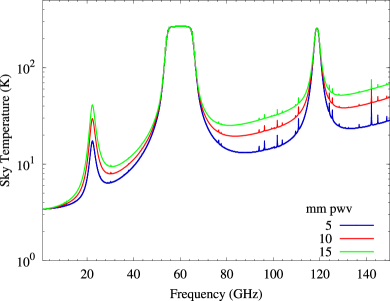
Figure 7: The atmospheric sky temperature at the zenith for a range of H₂O contents. The plots show the temperature for 5, 10 and 15 mm of precipitable water vapour and the standard sea level atmosphere (1013 mbar, 288 K). The plots are derived from the ATM model of Pardo et al. (2001)

The components of the atmospheric emission spectrum derived from the Atmospheric Transmission at Microwaves (ATM) model of Pardo et al. (2001) are shown in figure 7 for the frequency range 1–150 GHz. The sky brightness temperature is plotted for 5, 10 and 15 mm of precipitable water vapour (pwv) and a standard atmosphere at sea level pressure of 1013 mbar and a temperature of 288 K. It is seen that the O₂ line is optically thick ($\tau\geq 1$) at 60 GHz and the H₂O line is optically thick at 118 GHz. In addition to the H₂O lines, there is emission from the so called “excess water vapour absorption” (EWA) which appears as a broad frequency component that increases with frequency. The low opacity ranges in the total atmospheric spectrum are at $\leq 15$ GHz, $\sim 35$ GHz and $\sim 85$ GHz.

Sea level values of the pwv on clear days at low ambient temperature may be 5 mm, but is more commonly 10–20 mm. At heights of 2 km above sea level 5 mm is more usual (Danese & Partridge, 1989; Staggs et al., 1996).

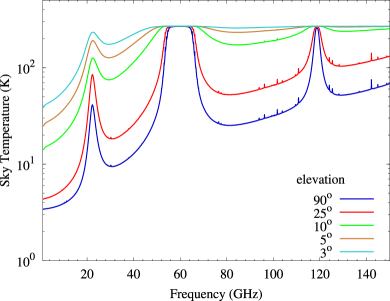
Figure 8: The atmospheric emission at elevations from 3^∘ to 90^∘ (zenith) in the frequency range 1–150 GHz the plots are derived from the ATM model of Pardo et al. (2001) and an H₂O content of 15 mm pwv.

$\lambda$	$\nu$	O2	H2O
(cm)	(GHz)	(K)	(K)
73	0.408	2.0	0.00
21	1.4	2.2	0.00
12	2.5	2.2	0.01
5.9	5.0	2.3	0.01
2.9	10	2.4	0.03
1.57	19	3.3	0.45
0.91	33	7.6	0.33
0.33	90	14.6	1.50

Table 3: The zenith atmospheric emission from O₂ and H₂O at sea level. Adapted from the observational data of Danese & Partridge (1989), Staggs et al. (1996) and Zhang et al. (2012). The O₂ emission is for the standard sea level atmosphere of 1013 mbar and a temperature of 288 K. The H₂O emission per mm pwv is given.

Table 3 gives direct observational data for the zenith emission at frequencies of potential interest here taken from the summary by Danese & Partridge (1989), which is based on the model of Waters (1976) and Smith (1982). The frequency bands are the standard ones allocated for radio astronomy; we also include 19 GHz, which is near the water line. These are augmented by 1.4 GHz data from Staggs et al. (1996) and Zhang et al. (2012). The O₂ emission is proportional to the local atmospheric pressure. The listed of values of the H₂O emission per mm of pwv can be used along with the local water vapour data to give the total H₂O emission. Table 4 gives the total (O₂ + H₂O + EWA) zenith emission for 10 mm pwv at selected frequencies.

The increase in atmospheric emission at lower elevation is of particular interest for this project. Fig. 8 shows the atmospheric spectrum for elevations of 3^∘, 5^∘, 10^∘, 25^∘ and 90^∘ (the zenith) estimated using the ATM code. Table 4 lists the total sky temperature for 10 mm pwv at elevations 3^∘, 5^∘, 10^∘, and 90^∘ at frequencies of interest for the current project. For example, at 10 GHz the sky temperature increases from 2.6 K at the zenith to 37 K and 54 K at elevations of 5^∘ and 3^∘ respectively. This extra emission will significantly increase the receiver system noise temperature at frequencies $\geq 10$ GHz. At the higher frequencies the spatial variation of the H₂O distribution may lead to unstable baselines in the recorded data. The O₂ distribution is relatively steady in comparison.

In a related fashion, the corresponding optical depth of the atmosphere at higher frequencies leads to significant absorption at lower elevations. For example, at 10 GHz the zenith absorption of 1 per cent increases to 6, 12 and 20 per cent at elevations of 10^∘, 5^∘ and 3^∘ respectively. When account is taken of these atmospheric emission and absorption effects, the choice of operating frequencies is $\leq 15$ GHz.

$\lambda$	$\nu$	Zenith $T$			Total $T$
(cm)	(GHz)	(K)			(K)
					Elevation
		O2	H2O		90∘	10∘	5∘	3∘
21	1.4	2.2	0.0		2.2	12.3	23	41
5.9	5.0	2.3	0.1		2.4	14.5	29	45
2.9	10.0	2.4	0.2		2.6	19.5	37	54
1.91	33	7.6	3.3		10.9	75.0	140	185
0.33	90	14.6	15.0		29.6	150	240	270

Table 4: Atmospheric emission as a function of elevation for selected frequencies in the range 1–100 GHz. The emission is given for 10 mm pwv. Data are from observations (Danese & Partridge, 1989; Staggs et al., 1996; Zhang et al., 2012) and from the modelling (Pardo et al., 2001; Smith, 1982; Waters, 1976; Crane, 1976).

5 The working system

A compact radio telescope suited to the observation of the Moon in proximity to the Sun is presented in this section.

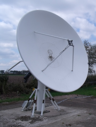
Figure 9: A photograph of the 3.7 m telescope showing the diagonal feed support arrangement

5.1 General requirements

The aim of the telescope is to acquire a set of scans of the sky temperature where the Sun and the Moon are located in the 24 hours prior to and after the time of New Moon at intervals of $\approx 1$ hour. As discussed in the previous sections, the ideal frequency for such observations is between 5 and 15 GHz. In this frequency range, the Sun brightness is $\sim 20$ dB above the Moon and the atmosphere is still relatively transparent. We have therefore chosen 10 GHz as the frequency for this project. Such frequencies is commonly used for satellite communications and the components (receivers, detectors, filters, etc.) are inexpensive and readily available.

In order to achieve its primary goal, the telescope must have a beamwidth small enough to resolve the Sun and the Moon even when in close proximity (less than few degrees). Given that the Moon moves $\approx 30$ arcmin per hour along the ecliptic with respect to the Sun and their minimum distance is 0^∘ (as during total solar eclipse), the beamwidth of the telescope must be $\approx 30$ arcmin. These considerations lead to a diameter of the antenna effective aperture $D\geq\lambda/\theta\approx 4$ m at the frequency of 10 GHz ($\lambda=3$ cm).

A second requirement derives from the strong sidelobe level associated with the much brighter Sun. The sidelobe level necessary to identify the Moon in the presence of the Sun, which is $\sim$ 50–100 times brighter at 10 GHz, is greater than 25 dB (a factor of 300) at a projected distance of 1^∘ to 2^∘ in the sky. This requires a polar diagram for the prime focus feed which tapers to $\leq-15$ dB at the edge of a parabolic reflector. As a result, the required reflector diameter may be larger in order to accommodate for the feed taper.

Figure 10: Diagram of the telescope detection system as implemented for the New Moon observations.

The telescope must be agile and have a fast scanning speed in order to obtain quasi-synchronous scans (snapshot) of the Sun and the Moon in celestial coordinates and avoid significant relative motion of the Moon during the observation. For a telescope with FWHM $\approx 30$ arcmin and given the Moon motion with respect to the Sun of 30 arcmin per hour, the scanning time must be less that 30 min to avoid significant motion of the Moon. For an observation performed 24 hours before or after closest approach, the angular separation of the Moon and Sun may be as large as $\approx 15^{\circ}{}$; depending on the scanning strategy, to cover an area of $15^{\circ}{}\!\times 15^{\circ}{}$ in size with a 30 arcmin beam leads to a minimum telescope pointing speed of no less than 30 arcmin per sec.

Parameter	Value
Reflector diameter	3.7 m
FWHM beamwidth	36 arcmin
Azimuth drive speed	$\geq 30$ arcmin per sec
Pointing accuracy	2 arcmin
Frequency	10.8 GHz
Bandwidth	1 GHz
$T_{sys}$ at zenith	100 K

Table 5: Telescope and receiver parameters.

5.2 The telescope

A telescope designed to observe the New Moon has been developed at the Jodrell Bank Observatory, UK (longitude $02^{\circ}{}18^{m}$ W, latitude $53^{\circ}{}14^{m}$ N). The telescope has been constructed in accordance with the requirements stated in the Sec. 5.1. The parameters of the telescope are given in Table 5.

The telescope receiver is a commercial room temperature satellite low-noise block downconverter (LNB) with an input radio frequency (RF) of 10.3 GHz to 11.3 GHz. The LNB contains the low-noise amplifier (LNA), a local oscillator (LO) and a mixer to down-convert the input frequency to the Intermediate Frequency (IF) of 950 MHz to 2.0 GHz. After a further 20 dB amplification, the IF signal is converted into a DC voltage by a power-law detector diode. The DC level is then amplified using two operational amplifiers in the inverting configuration and filtered using a RC low-pass filter with a cut-off frequency of 150 kHz. The two DC amplifiers have $-4.7$ and $-10$ gain respectively. A commercial data acquisition system (DAQ) containing an analogue to digital 16 bits card measures the filtered DC at a sampling rate of up to 25 kHz. Fig. 10 shows the telescope detection system; the diagram includes the LNB power supply (PSU) and an IF switch used to divert the RF signal to a spectrum analyzer for testing.

The telescope reflector is a parabolic dish 3.7 m in diameter. It is illuminated with a horn feed located at the primary focus to give a beam with sidelobes more than $20$ dB lower than the main beam. The feed and receiver system are supported at the dish focus by four metallic cylindrical legs 7 cm in diameter and 1.5 m in length. Fig. 9 is a photograph of the telescope; it shows the 3.7 m reflector, the receiver and the diagonal feed support arrangement.

The telescope pointing is obtained directly from two 24-bit absolute rotary encoders on the azimuth and elevation axes. The Sun was used to test the telescope pointing accuracy and was found to be good to $\approx 2$ arcmin using this simple method. This value is sufficiently small given the large telescope beam. The telescope drive speed is $\approx 30$ arcmin per second in both azimuth and elevation directions.

At the frequency of 10.8 GHz and for a 3.7 m effective aperture antenna, the expected main beam FWHM is $\approx 30$ arcmin. The beam FWHM was measured on a geostationary satellite to be $36\pm 3$ arcmin. This value was confirmed by the Moon and Sun measurements (see below).

5.2.1 Data acquisition and mapping

The recorded time-ordered-data include the telescope position, the receiver output voltage and the time. The UTC time is obtained from an NTP server using the GPS system as the primary timing source. A sampling rate of 50–100 Hz for both the receiver DC voltage and telescope position gives more than adequate redundancy in the data streams.

The telescope is capable of recording a $15^{\circ}{}\!\times 15^{\circ}{}$ map of the sky signal around the Sun and the Moon every 30–40 minutes at the time of New Moon. The scanning strategy is to cover the required sky area with a series of azimuth scans at intervals of 15 arcmin in elevation which gives a sky sampling at the Nyquist rate for a 36 arcmin beam. Each 15^∘ azimuth scan takes 20 sec at the scan rate of 30 arcmin per sec. With a turn-around of 10 sec to account for deceleration and reacceleration, the net time for a scan is 30 sec. This satisfies the requirement to complete the map of the Sun/Moon within 30 min.

A baseline is removed from each scan before it is incorporated into the final map. The map is obtained by simple binning of the signal into a two dimensional array. Further destriping of the map can be performed off-line.

The map can be displayed in celestial coordinates (RA and Dec) for the purpose of displaying the passage of the Moon past the Sun when determining the true time of New Moon (Bruin, 1977; Ilyas, 1994; Yallop, 1997; Hoffman, 2003).

5.2.2 Polar diagram measurements

The beam shape is well defined with high signal-to-noise using the Sun. A map of the sidelobe structure using observations made on 28 May 2012 is shown in Fig. 11. Both the circular inner diffraction sidelobes and the diagonal scattering sidelobes can be seen. The diffraction lobe is at a radius of 1^∘50^′. An inner diffraction lobe is suggested at a radius of $\approx 1$^∘ embedded in the main beam as convolved with the Sun. The diagonal sidelobes produced by the scattering of Earth and Sun radiation into the prime beam can be traced out to a radius of 7^∘ from the beam centre where the amplitude is 0.3 per cent ($-25$ dB) of the main beam response.

Figure 11: Map of the sidelobe structure on the Sun observed 17:05 UT on 28 May 2012 at an elevation of 27^∘. Contours are at 0.1, 0.2, 0.4, 1.4, 6.3, 20 and 63 per cent of the peak (the lowest 3 contours correspond to $-30$, $-27$, $-24$ dB). Both the circular diffraction lobe and the diagonal scattering sidelobe structures can be seen

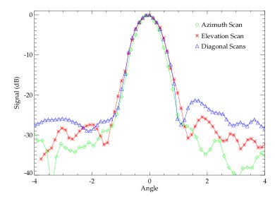
Figure 12: Plot of the beam response showing the main beam and sidelobes for the Sun on 28 May 2012 as seen in Fig. 11. The curves are the azimuth (green diamonds) and elevation (red stars) scans and the average of the two diagonal direction scans (blue triangles).

The amplitude of the sidelobe structure is quantified in Fig. 12 on a logarithmic dB scale. The elevation and azimuth cuts show that the diffraction lobes at a radius of 1^∘50^′ are $-27$ dB compared to the peak. The average diagonal cut shows variations of $-25$ to $-28$ dB extending from 1^∘ 30^′ out to 7^∘ radius. Beyond that radius the level falls further to a level of $\leq-30$ dB (0.1 per cent), comparable to the noise level at the pixel scale of the map.

It can be seen when comparing observations of the Sun on different days (Figs. 11 and 13) that the sidelobes are sufficiently stable and a sidelobe template of the Sun can be removed from the map. This would more clearly show the Moon and the Sun as convolved with the 36 arcmin primary beam without the confusion of Sun sidelobes.

5.3 Observation of the Sun and Moon at New Moon on 21 May 2012

An observation of the Sun and Moon some 4 hours before sunset on 21 May 2012 is shown in Figure 13. Contours are given at the same levels as in Figure 11. The sidelobe levels are very similar to those on the 28 May 2012 when the elevation was similar. This has implications for the possibility of developing an algorithm for subtracting a sidelobe template from the observations in order improve the Moon visibility against the brighter Sun as described in Sec. 5.2.2. At low elevations ($\leq 10$^∘) account would have to be taken of the greater scattering of Earth radiation from the feed supports as well as atmospheric absorption and refraction. These latter effects are calculable and small.

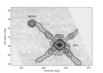
Figure 13: A map of the Sun and Moon on 21 May 2012 near the time of New Moon. The Sun was observed at 16:27 UT; the Moon at 16:36 UT. Contours are at 0.1, 0.2, 0.4, 1.4, 6.3, 20, and 63 per cent of the Sun peak. The sidelobe levels may be compared directly with those in Figure 11 for 28 May 2012 observation.

The Moon is clearly visible even though it lies close to a diagonal lobe. Cuts across the Moon parallel and perpendicular to the diagonal lobe are shown in Fig. 14. The cut parallel to the sidelobe is $-4$ to $-5$ dB relative to the perpendicular cut. The parallel cut shows that the Moon was 1.37 $\pm$ 0.03 per cent of the Sun, indicating that the Sun was $73.0\pm 2.2$ times brighter than the Moon on 21 May 2012. The Moon is clearly detected at about 13 dB (factor of 20) above the sidelobe structures. The effective noise level in Fig. 11 is $\approx 0.03$ per cent relative to the Sun.

Figure 14: Cuts through the centre of the Moon on 21 May 2012 parallel (full line) and perpendicular (dashed line) to the diagonal lobe direction. Amplitudes are given as per centage of the Sun.

5.4 Comparison of Sun to Moon ratio with previous data

The observed ratio of 73 for the Sun-to-Moon emission at 10.8 GHz can be compared with the value predicted from the literature as outlined in Sections 2 & 3 and Tables 1 & 2 of this paper. The relevant input data for this calculation of the New Moon on 21 May 2012 are given on Table 6.

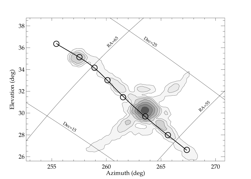
Figure 15: The map of 16 hr 36 min UT on 21 May 2012 with suporimposed celestial coordinates. The path of the Moon relative to the Sun in celestial coordinate is shown at 4 hour intervals for the previous 24 hours. The Moon passed closest to the Sun at 00 hr 09 min UT.

Sun 21 May 2012
Mean diameter	31.99 arcmin
Diameter on observation day	31.66 arcmin
Quiet Sun (SS max)		16,600 K
Quiet Sun (SS min)		12,600 K
Quiet Sun on 21 May 2012		14,600 K
Sunspot number $R=$ 71
Sunspot emission		1,500 K
Expected $T_{b}$		16,100 K
Sun area correction	$-2.1$ per cent
Corrected Tb		15,800 K
Moon 21 May 2012
Mean diameter	29.50 arcmin
Diameter 21 May 2012	30.09 arcmin
Moon mean Tb		216 K
First harminic correction	$-11$ K	205 K
Moon area correction	+4.0 per cent
Corrected Tb		213 K
Expected ratio Sun/Moon	$74.2\pm 7.4$
Observed ratio Sun/Moon	$73.0\pm 2.2$

Table 6: Estimation for the Sun and the Moon brightness temperature at 10 GHz on 21 May 2012. The Sun and Moon are observed at similar elevations and so there is no effect on the Sun/Moon ratio.

The quiet Sun brightness temperature for 21 May 2012 is taken as the average of the sunspot maximum and minimum values, namely 14,600 K. The sunspot emission for a sunspot number $R=71$ is 1,500 K at 10 GHz (Table 1). The Sun diameter on 21 May 2012 (31.66 arcmin) is less than its mean diameter (31.99 arcmin) used for the solar data in Table 1. This leads to an area correction of $-2.1$ per cent which gives a reduction of the effective T_b from 16,100 K to 15,800 K.

The Moon mean brightness temperature at 10 GHz is 216 K with a correction of $-11$ K for a first harmonic phase lag of 40^∘ at the time of New Moon. On correction for the Moon diameter to 21 May 2012, the predicted brightness temperature of the Moon is 213 K.

The predicted ratio Sun-to-Moon for 21 May 2012 is $74\pm 7$. The uncertainty is mainly in the solar value which conservatively is 10 per cent. This ratio may be compared with the observed value for that day of $73.0\pm 2.2$. This agreement confirms that the Sun and Moon parameters given in Tables 1&2 are a reliable guide for estimating the relative brightness of the Sun and Moon.

5.5 Estimation of time of New Moon

The time of New Moon is defined as the time of minimum elongation of the Moon from the Sun in celestial coordinates (Bruin, 1977; Hoffman, 2003; Ilyas, 1994). Figure 15 shows this situation for the New Moon on 21 May 2012 as seen from Jodrell Bank Observatory (longitude 00^h09${}^{m}\!$.2, latitude 53^∘14^′). The Moon and Sun positions are for 16 hr 36 min UT and 16 hr 26 min UT respectively. The movement of the Moon in celestial coordinates is shown at 4 hr intervals during the previous 24 hours.

The plot shows that the Moon past in front of the Sun 16 hr 25 min previous to the observation shown here, namely at 00 hr 12 min UT on 21 May 2012. During this 16 hr 25 min interval, the Sun will have moved +2${}^{m}\!$.5 in RA, thus making the true New Moon at 00 hr 09 min as seen from Jodrell Bank Observatory. This agrees with the time of an annular eclipse of the Sun which occurred at 00 hr00 min UT.

6 Discussion and conclusions

6.1 Review of the aims

We have shown that it is possible to design a radio telescope for direct observation of the time of New Moon. Optimal frequencies are in the range 5–15 GHz where the ratio of the Sun to Moon is 50–100 ($\leq$ 20 dB), so as not to be confused by the sidelobes of the telescope.

At these frequencies the angular diameter of the Sun approaches the optical value of 0^∘.5. The Moon angular diameter is 0^∘.5 at all frequencies. A telescope of moderate size gives a beamwidth of 0^∘.5 which is suitable for clearly separating the Sun and Moon. The emission from the Earth’s atmosphere is manageable at the low elevation required by the traditional methods of sighting the New Moon.

6.2 The radio telescope system

A system operating at 10.8 GHz has been built to demonstrate the practicability of detecting the Moon as it passes the Sun at the time of New Moon. The telescope sidelobes are $\approx-23$ dB as compared with $-18.6$ dB for the Moon-to-Sun ratio. These sidelobes are shown to be stable and can be accounted for in the analysis by subtracting a beam template of the Sun sidelobes.

At 10.8 GHz the New Moon observations can be followed down to an elevation of $\approx$3^∘ where the atmospheric emission increases the system noise by $\approx 40$ K and the attenuation of the Sun and the Moon signals by $\approx 15$ per cent (0.6 dB).

The telescope scanning strategy and pointing accuracy were shown to give a 15^∘$\times$15^∘ map of the Moon-Sun field in 30 min. The aims for the project set out in Sec 5.1 and 6.1 are achieved.

6.3 Measurements on 21 May 2012

The setting Sun-Moon field was observed 16 hours after the annular eclipse of the Sun at 00 hr 00 min UT on 21 May 2012. The Sun/Moon ratio was $73.0\pm 2.2$ in agreement with the data from the literature given in the Tables 1 and 2. It was found using the observed images that the Moon can be clearly distinguished from the Sun for any angular distance above $\approx 2$^∘. Fig. 15 is a plot of the path of the Moon relative to the Sun in the RA-Dec system for the previous 24 hours which shows that the New Moon would have occurred at 00 hr 09 min as seen from Jodrell Bank Observatory.

6.4 Conclusions – the potential of the radio method

We have made a successful test of a radio method of directly observing the time of New Moon. It has the advantage over the optical (naked eye or binocular) method of sighting the New Moon in that at radio frequencies (5–15 GHz) the Moon is $\sim 10^{-2}$ of the brightness of the Sun as compared with $10^{-5.5}$ for optical frequencies. Furthermore this method is essentially independent of the weather in the form of water clouds or atmospheric dust. Observations of the Moon are possible at elevations down to $\approx 3^{\circ}{}$ where the atmospheric opacity is $\approx 15$ per cent and the emission is less than the receiver system temperature at the radio frequency of 10.8 GHz chosen for this project.

The radio approach can be used at any time of day from sunrise to sunset. The present approach is to map the Sun and the Moon field every 30 min for 24 hr either side of the true New Moon. The resulting “movies” will trace the locus of the Moon as it passes the Sun at 30 min intervalls which corresponts to 0^∘$\!.25$ steps. At a single site there is a period of $12\pm 2$ hours when the Moon/Sun system is beneath the horizon. Accordingly, observations near sunset and sunrise are important for interpolating the time of closest approach if it occurs during the night time. The time of true New Moon, when the Moon is nearest to the Sun, is then directly evident. In principle, this could change the beginning of the lunar calendar month by as much as one day, since it begins when the Moon is observed at the first sunset after conjunction.

References

- Bruin (1977) Bruin F., 1977, Vistas in Astronomy, 21, Part 4, 331
- Christiansen & Warburton (1955) Christiansen W. N., Warburton J. A., 1955, Australian Journal of Physics, 8, 474
- Christiansen et al. (1957) Christiansen W. N., Warburton J. A., Davies R. D., 1957, Australian Journal of Physics, 10, 491
- Covington (1974) Covington A. E., 1974, JRASC, 68, 31
- Covington & Medd (1954) Covington A. E., Medd W. J., 1954, JRASC, 48, 136
- Cox (2000) Cox A. N., ed., 2000, Allen’s Astrophysical Quantities. Springer–Verlag, New York
- Crane (1976) Crane R. K., 1976, in Astrophysics. Part B: Radio Telescopes, Meeks M. L., ed., pp. 136–141
- Danese & Partridge (1989) Danese L., Partridge R. B., 1989, ApJ, 342, 604
- Dodson et al. (1954) Dodson H. W., Hedeman E. R., Covington A. E., 1954, ApJ, 119, 541
- Hagfors (1970) Hagfors T., 1970, Radio Science, 5, 189
- Harrison et al. (2000) Harrison D. L. et al., 2000, Monthly Notices of the Royal Astronomical Society, 316, L24
- Hathaway et al. (1994) Hathaway D., Wilson R., Reichmann E., 1994, Solar Physics, 151, 177
- Heiken et al. (1991) Heiken G. H., Vaniman D. T., French B. M., 1991, Lunar Sourcebook - A User’s Guide to the Moon. Cambridge University Press
- Hoffman (2003) Hoffman R. E., 2003, MNRAS, 340, 1039
- Ilyas (1994) Ilyas M., 1994, Quarterly Journal of the Royal Astronomical Society, 35, 425
- Krotikov & Pelyushenko (1987) Krotikov V. D., Pelyushenko S. A., 1987, Soviet Astronomy, 31, 216
- Kundu (1965) Kundu M. R., 1965, Solar Radio Astronomy. John Wiley and Sons, New York
- Linsky (1973) Linsky J. L., 1973, ApJS, 25, 163
- Pardo et al. (2001) Pardo J., Cernicharo J., Serabyn E., 2001, Antennas and Propagation, IEEE Transactions on, 49, 1683
- Poppi et al. (2002) Poppi S., Carretti E., Cortiglioni S., Krotikov V. D., Vinyajkin E. N., 2002, in American Institute of Physics Conference Series, Vol. 609, Astrophysical Polarized Backgrounds, Cecchini S., Cortiglioni S., Sault R., Sbarra C., eds., pp. 187–192
- QUIET Collaboration et al. (2012) QUIET Collaboration et al., 2012, ArXiv e-prints
- Smith (1982) Smith E. K., 1982, Radio Science, 17, 1455
- Staggs et al. (1996) Staggs S. T., Jarosik N. C., Wilkinson D. T., Wollack E. J., 1996, ApJ, 458, 407
- Troitskii & Tikhonova (1970) Troitskii V. S., Tikhonova T. V., 1970, Radiophysics and Quantum Electronics, 13, 981
- Waters (1976) Waters J. W., 1976, in Astrophysics. Part B: Radio Telescopes, Meeks M. L., ed., p. 142
- Yallop (1997) Yallop B. D., 1997, Technical notes N. 69, HM Nautical Almanach Office
- Zhang et al. (2012) Zhang X.-Z., Gray A., Su Y., Li J.-D., Landecker T., Zhang H.-B., Li C.-L., 2012, Research in Astronomy and Astrophysics, 12, 1297
- Zheng et al. (2009) Zheng Y. C., Bian W., Su Y., Feng J. Q., Zhang X. Z., Liu J. Z., Zou Y. L., 2009, Geochimica et Cosmochimica Acta Supplement, 73, 1523