Photometric type Ia supernova surveys in narrow band filters

Abstract

We study the characteristics of a narrow band type Ia supernova survey through simulations based on the upcoming Javalambre Physics of the accelerating universe Astrophysical Survey (J-PAS). This unique survey has the capabilities of obtaining distances, redshifts, and the SN type from a single experiment thereby circumventing the challenges faced by the resource-intensive spectroscopic follow-up observations. We analyse the flux measurements signal-to-noise ratio and bias, the supernova typing performance, the ability to recover light curve parameters given by the SALT2 model, the photometric redshift precision from type Ia supernova light curves and the effects of systematic errors on the data. We show that such a survey is not only feasible but may yield large type Ia supernova samples (up to 250 supernovae at $z<0.5$ per month of search) with low core collapse contamination ($\sim 1.5$ per cent), good precision on the SALT2 parameters (average $\sigma_{m_{B}}=0.063$, $\sigma_{x_{1}}=0.47$ and $\sigma_{c}=0.040$) and on the distance modulus (average $\sigma_{\mu}=0.16$, assuming an intrinsic scatter $\sigma_{\mathrm{int}}=0.14$), with identified systematic uncertainties $\sigma_{\mathrm{sys}}\la 0.10\sigma_{\mathrm{stat}}$. Moreover, the filters are narrow enough to detect most spectral features and obtain excellent photometric redshift precision of $\sigma_{z}=0.005$, apart from $\sim$ 2 per cent of outliers. We also present a few strategies for optimising the survey’s outcome. Together with the detailed host galaxy information, narrow band surveys can be very valuable for the study of supernova rates, spectral feature relations, intrinsic colour variations and correlations between supernova and host galaxy properties, all of which are important information for supernova cosmological applications.

1 Introduction

Supernovae (SNe) and their relations with their surrounding environment have been an active field of study for decades. Their progenitors and explosion mechanisms are not fully known and understood, nor are all their possible variations, sub-classes and behaviours (Hamuy et al., 2000; Sullivan et al., 2006; Leonard, 2007; Xavier et al., 2013). On top of that, SNe play a key role in other scientific fields like chemical evolution of intra and intergalactic medium (Wyse & Silk, 1985; Zaritsky et al., 2004; Scannapieco et al., 2006), star formation rate in galaxies (Tsujimoto et al., 1999; Yungelson & Livio, 2000; Seo & Kim, 2013), energetics of the interstellar medium (Chevalier, 1977), galaxy cluster density and temperature profiles (Suginohara & Ostriker, 1998; Voit & Bryan, 2001), and on measurements of the cosmological expansion history of the universe (Riess et al., 1998; Perlmutter et al., 1999; Conley et al., 2011; Sullivan et al., 2011). Many of these subjects are interconnected, and a better understanding of one is likely to positively influence the other.

SN studies are made more difficult due to their rarity and their transient nature: SN rates are of order unity per galaxy per century and they are visible only for a couple of months (Carroll & Ostlie, 1996). Fortunately, their cosmological importance have driven and continues to drive astrophysical surveys that can amass a relatively large number of such events. These surveys – such as the Supernova Legacy Survey (SNLS, Pritchet et al., 2005; Astier et al., 2006), the ESSENCE supernova survey (Miknaitis et al., 2007), the Sloan Digital Sky Survey (SDSS, York et al., 2000; Frieman et al., 2008), the Dark Energy Survey (DES, DES Collaboration, 2005; Bernstein et al., 2012), Pan-Starrs (Kaiser et al., 2010) and the Large Synoptic Survey Telescope (LSST, Ivezic et al., 2008; LSST collaboration, 2009) – are broad band photometric surveys backed up by spectroscopic measurements. An appropriately time-distributed sequence of observations in a few broad band filters can provide a good measurement of the SN light curves up to high redshifts, while spectroscopy was indispensable for typing the SN and measuring its redshift.

Even though these projects could obtain images of a huge amount of SN candidates, their typing (a fundamental part in a SN program) was strongly based on their spectral features. While secure, this method is costly and time consuming, therefore it severely limits the SN sample sizes, specially since SN science must share time with different surveys goals. For instance, SDSS database contains near 660 spectroscopically confirmed SNe out of a total of $\sim 4650$ photometric SNe candidates (14 per cent), and DES expects to measure the spectra of 800 type Ia SNe from a total of 4000 SNe Ia with host galaxy spectroscopy (20 per cent) (Bernstein et al., 2012).

With this bottleneck in mind, a lot of effort was placed on photometrically typing SN candidates (e.g. Kessler et al., 2010b) and a lot of progress was achieved in this field (e.g. Sako et al., 2011). Even though typing can be reasonably good for SNe Ia without spectroscopy, a precise redshift prior is still needed in order to get good constraints on SN properties (specially colour), and this prior has to be obtained with spectroscopic measurements of the SN’s host galaxy. This change in spectroscopy target (from the SNe to their hosts) facilitates the observations by allowing the measurements to be made well after the SNe have vanished, but it still presents a bottleneck for SN samples. From SDSS, $\sim 2500$ of the SNe without direct spectroscopic measurement also did not have spectroscopy from its host. These purely photometric SN samples will grow in the future as new surveys such as the LSST are expected to detect and measure the light curve of $\sim 10^{7}$ SNe (LSST collaboration, 2009).

Spectroscopy is not only beneficial for SN light curve fitting and for measuring its redshift: it also conveys information about the SN properties. For instance, studies have indicated that SN Ia spectral features like the width of the SiII line and various flux ratios can be used to improve distance measurements (Nugent et al., 1995; Bongard et al., 2006; Hachinger et al., 2006; Bronder et al., 2008; Foley et al., 2008; Bailey et al., 2009; Chotard et al., 2011; Nordin et al., 2011). On top of that, SN Ia spectroscopy can help us to distinguish between various models for their luminosity intrinsic scatter (Kessler et al., 2013). These measurements do not require high resolution spectra since the SN absorption features are reasonably large (for a review, see Filippenko, 1997).

SN science benefits also from spectroscopy of the SN host galaxies. An accurate measurement of the hosts properties – or, even better, of the environment in the vicinity of the SNe – will help to pin down their possible progenitors (Galbany et al., 2012). Besides, the SN environment was shown to correlate with their rates and properties (Sullivan et al., 2006; Dilday et al., 2010; Gupta et al., 2011; Li et al., 2011; Xavier et al., 2013), which are important information for stellar and chemical evolution of galaxies and galaxy clusters, and for cosmological distance measurements (Sullivan et al., 2010; Lampeitl et al., 2010).

Given the importance of spectroscopic data and the challenges of obtaining it in large scale, we investigate the expected characteristics of a photometric SN Ia survey performed with a set of contiguous narrow band filters. Filters with transmission functions about 100–200 Å  wide still have enough resolution to detect almost every SN spectral feature. Since it acts as a low resolution spectrograph equipped with an integral field unit (IFU), all SNe detected by this type of survey automatically have their spectra measured. Moreover, it naturally yields rich information about their local environments.

Figure 1: SN Ia spectral surface at redshift $z=0.25$ convolved with top-hat functions $T(\lambda)$ 1000 Å  (left panel) and 100 Å  wide (right panel), representing the resolution attainable with broad and narrow band filters, respectively. The epoch $t_{\mathrm{obs}}$ is given in days from maximum luminosity and the flux density $f_{\lambda}$ is in arbitrary units. SN observations can be represented as $N$ sampling points at specific epochs and filters central wavelengths $\{(\lambda_{1},t_{1}),\ldots,(\lambda_{N},t_{N})\}$. A typical broad band sampling and a possible narrow band sampling are shown in the left and right panels, respectively. Filters with bandwidths $\sim 100$ Å  can detect practically all SN spectral features while filters $\sim 1000$ Å  wide can only detect large scale features.

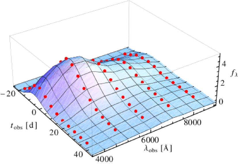
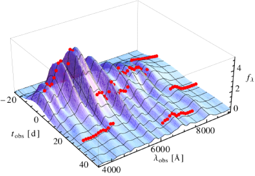
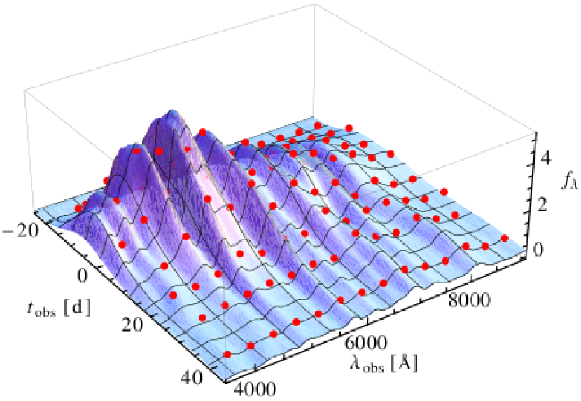
The main features of a narrow band SN survey are best described with the help of Fig. 1, which presents the spectral energy distribution of a SN Ia as a function of time $f_{\lambda}(\lambda_{\mathrm{obs}},t_{\mathrm{obs}})$ – called spectral surface – with typical wavelength resolutions for broad band (left panel) and narrow band filters (right panel). Measurements can be interpreted as sampling these surfaces at specific points, and the amount of information available for a narrow band survey is clear. For instance, while for a broad band survey the SN redshift must be inferred from the position of a wide peak, it can be inferred from the position of all the spectral peaks and troughs in the case of a narrow band survey. Fig. 1 also emphasises that the relevant SN quantities to be well sampled and constrained are not individual light curves (spectral surface slices at fixed $\lambda$) but the entire collection of correlated light curves (i.e. the spectral surface itself). The individual light curve perspective is common in broad band SN surveys given they can only sample the spectral surface (Fig. 1, left panel) at 1–5 different wavelengths. Since narrow band surveys may sample the spectral surface (Fig. 1, right panel) at 20–60 different wavelengths, a large sampling in the same wavelength is not as important and one or two might suffice – provided the observations in different wavelengths are also appropriately distributed in time.

In this paper we make forecasts of SN Ia data obtainable with a narrow band filter survey by simulating and fitting light curves with the SALT2 model (Guy et al., 2007) as implemented by the snana software package (Kessler et al., 2009b), using the Javalambre Physics of the accelerating universe Astrophysical Survey (J-PAS, Benitez et al., 2014) as our fiducial survey. We estimate the performance of such a narrow band survey regarding the amount of observable SNe Ia, their average error and bias on various parameters, their redshift distribution and their typing purity and completeness, and compared with results for broad band surveys, namely SDSS and DES. Medium band surveys were already performed in the past [e.g. the COMBO-17 survey (Wolf et al., 2003) used 12 filters about 220 Å  wide and the ALHAMBRA survey (Moles et al., 2008; Benitez et al., 2009b; Molino et al., 2014) used 20 filters $\sim 310$ Å  wide], while narrow band surveys – J-PAS and PAU (Benitez et al., 2014; Martin et al., 2014) – are already being implemented. Besides, future spin-offs like a southern copy of J-PAS are under planning.

The outline of this paper is as follows: in section 2 we describe all the inputs we used to simulate the SN data, starting from light curve models and their allowed range of parameters (section 2.1). Sections 2.2 and 2.3 describe our fiducial survey, including its filter system and observing strategy. Host galaxy inputs and various noises estimates are described in sections 2.4 and 2.5. Our simulation results are presented in section 3: the expected number of SNe per season and its redshift distribution; the flux measurement signal-to-noise ratio in each redshift and filter (section 3.1); the SN typing efficiency, SN Ia light curve parameters recovery and distance measurement precision (sections 3.2 and 3.3); and the quality of redshift inference from SN Ia light curves (section 3.4). A few suggestions for optimising a narrow band SN survey are presented in section 4, and some systematic uncertainties are discussed in section 5. Our conclusions and a summary of our main findings are presented in section 6.

2 Simulation characteristics

Snana can make realistic simulations of supernova surveys by generating different SN light curves at various redshifts according to a specified rate, then applying noise to the data – based both on their intrinsic properties and on the survey apparatus – and selecting the actually detected SNe based on defined selection cuts and on the survey design. The simulated data can then be typed and fitted just like real data.

To perform the simulations, the following inputs are required: a SN light curve model and distributions for its parameters; a SN rate as a function of redshift; a library of potential host galaxies, used to introduce extra noise and to possibly supply a redshift prior to the SNe; either the SN position or the value of the Milky Way excess colour in order to calculate the Galactic extinction; the filters transmission functions; an observation schedule listing the days and filters used, along with the photometric conditions (zero points, sky noise, CCD readout noise and point spread function); the area covered by the survey; and eventual selection cuts that can be applied to the data. These are described in detail below. We also briefly describe the typing and fitting methods used by the snana package.

2.1 Light curve models

Table 1: Light curves and spectra used as templates for simulating CC-SNe. The columns present, from left to right: a template identification; its type; the fraction of the simulated CC-SN light curves generated using each template; the mean absolute magnitude at peak in B band, in the supernova rest-frame, and the standard deviation $\sigma_{M_{B}}$ of the light curves simulated with each template. These are the default snana templates; all values (Frac., $M_{B}$ and $\sigma_{M_{B}}$) were set to match those reported in Li et al. (2011).

Template ID	Type	Frac.	$M_{B}$	$\sigma_{M_{B}}$
SDSS-000018	IIP	0.0246	-17.11	1.050
SDSS-003818	IIP	0.0246	-15.09	1.050
SDSS-013376	IIP	0.0246	-15.46	1.050
SDSS-014450	IIP	0.0246	-16.16	1.050
SDSS-014599	IIP	0.0246	-16.06	1.050
SDSS-015031	IIP	0.0246	-15.25	1.050
SDSS-015320	IIP	0.0246	-15.61	1.050
SDSS-015339	IIP	0.0246	-16.32	1.050
SDSS-017564	IIP	0.0246	-17.01	1.050
SDSS-017862	IIP	0.0246	-15.68	1.050
SDSS-018109	IIP	0.0246	-16.02	1.050
SDSS-018297	IIP	0.0246	-15.28	1.050
SDSS-018408	IIP	0.0246	-15.29	1.050
SDSS-018441	IIP	0.0246	-15.37	1.050
SDSS-018457	IIP	0.0246	-15.65	1.050
SDSS-018590	IIP	0.0246	-14.52	1.050
SDSS-018596	IIP	0.0246	-15.80	1.050
SDSS-018700	IIP	0.0246	-14.32	1.050
SDSS-018713	IIP	0.0246	-15.25	1.050
SDSS-018734	IIP	0.0246	-14.84	1.050
SDSS-018793	IIP	0.0246	-16.42	1.050
SDSS-018834	IIP	0.0246	-15.71	1.050
SDSS-018892	IIP	0.0246	-15.44	1.050
SDSS-020038	IIP	0.0246	-17.04	1.050
SDSS-012842	IIn	0.0200	-17.33	1.500
SDSS-013449	IIn	0.0200	-16.60	1.500
Nugent+Scolnic	IIL	0.0800	-16.75	0.640
CSP-2004gv	Ib	0.0200	-16.69	0.000
CSP-2006ep	Ib	0.0200	-18.51	0.000
CSP-2007Y	Ib	0.0200	-15.53	0.000
SDSS-000020	Ib	0.0200	-16.14	0.000
SDSS-002744	Ib	0.0200	-15.99	0.000
SDSS-014492	Ib	0.0200	-16.93	0.000
SDSS-019323	Ib	0.0200	-16.11	0.000
SNLS-04D1la	Ibc	0.0167	-15.84	1.100
SNLS-04D4jv	Ic	0.0167	-14.50	1.100
CSP-2004fe	Ic	0.0167	-15.66	1.100
CSP-2004gq	Ic	0.0167	-14.93	1.100
SDSS-004012	Ic	0.0167	-15.84	1.100
SDSS-013195	Ic	0.0167	-15.63	1.100
SDSS-014475	Ic	0.0167	-16.53	1.100
SDSS-015475	Ic	0.0167	-14.43	1.100
SDSS-017548	Ic	0.0167	-16.34	1.100

For simulating Core Collapse SNe (CC-SNe) we used the spectral templates available in the snana package, listed in Table 1, which were based on objects observed by various surveys. Table 1 also shows the fraction of simulated CC-SNe that was drawn from each template, the absolute AB magnitude in the B band, in the supernova rest-frame, used to normalise it and a coherent (same for all epochs and wavelengths) random Gaussian deviation applied to the magnitude in each simulation of that template. These values were based on the work of Li et al. (2011). The extinction caused by host galaxy dust is modelled with the curve from O’Donnell (1994), a fixed ratio of total to selective extinction $R_{V}=2.22$ and an extinction at band V, $A_{V}$, drawn from a distribution $f(A_{V})=\exp(-A_{V}/0.334)$, limited to values $-1<A_{V}<1$.

For simulating and fitting SN Ia light curves, we used the SALT2 model which is adequate for narrow band filters since it returns sufficiently high resolution ($\sim 60$ Å) spectra for each epoch (Guy et al., 2007). Since a narrow band survey is likely to detect more variation in the light curves and spectra than current models can predict, these are to be understood as general guides to how well such surveys can perform.

SALT2 is an observer frame spectral model based on five parameters: the redshift $z$, a time of maximum luminosity $t_{0}$, a colour term $c$, a principal component factor $x_{1}$ which can be roughly interpreted as a stretch parameter, and an overall normalisation $x_{0}$, which can be translated into an apparent magnitude $m_{B}$ at peak in the SN rest-frame $B$ band. The observed spectral flux density $f_{\lambda}$ for a given epoch $t_{\mathrm{obs}}$ and wavelength $\lambda_{\mathrm{obs}}$ is given by:

$$f_{\lambda}(\lambda_{\mathrm{obs}},t_{\mathrm{obs}})=\frac{x_{0}}{1+z}\left[M_{0}\left(\lambda,t\right)+x_{1}M_{1}\left(\lambda,t\right)\right]e^{cC\left(\lambda\right)}\;,$$ (1)

where $\lambda$ and $t$ are the rest-frame wavelength and time from maximum, given by: $\lambda=\lambda_{\mathrm{obs}}/(1+z)$ and $t=(t_{\mathrm{obs}}-t_{0})/(1+z)$. $M_{0}(\lambda,t)$ is a rest-frame average spectral surface (it gives you the average spectrum for each epoch $t$); $M_{1}(\lambda,t)$ is a principal component that accounts for the main deviations from $M_{0}$; and $C(\lambda)$ is a time-independent colour law that accounts for both intrinsic colour variations and dust extinction by the host galaxy.

For each simulated SN, the redshift $z$ is randomly drawn according to the survey volume at each $z$ slice and to the CC-SN (Kessler et al., 2010b) and SN Ia (Dilday et al., 2008) rates below:

$$\frac{\mathrm{d}N_{CC}}{\mathrm{d}z}=6.8\times 10^{-5}(1+z)^{3.6}h_{70}^{3}\;\mathrm{Mpc^{-3}yr^{-1}}\;,$$ (2)

$$\frac{\mathrm{d}N_{Ia}}{\mathrm{d}z}=2.6\times 10^{-5}(1+z)^{1.5}h_{70}^{3}\;\mathrm{Mpc^{-3}yr^{-1}}\;,$$ (3)

where $h_{70}=H_{0}/(70\mathrm{\;km\;s^{-1}\;Mpc^{-1}})$ and $H_{0}$ is the Hubble constant. The $x_{1}$ and $c$ parameters are drawn from Gaussian distributions with zero mean and standard deviations of 1.3 and 0.1, respectively, but constrained to the range $-5<x_{1}<5$ and $-0.4<c<0.4$. The time of maximum $t_{0}$ is drawn from a uniform distribution, and $x_{0}$ is calculated from the formula:

$$x_{0}=10^{-0.4(m_{B}-M-30)}\;,$$ (4)

$$m_{B}-M=\mu-\alpha x_{1}+\beta c\;,$$ (5)

where $M$ is an average absolute magnitude, $\alpha$ and $\beta$ are positive constants that account for the fact that SNe Ia with broader light curves ($x_{1}>0$) are usually brighter while redder SNe Ia ($c>0$) are usually dimmer. When simulating SNe Ia, these three quantities were fixed to $M=-19.365$, $\alpha=0.11$ and $\beta=2.60$ (Richardson et al., 2002; Kessler et al., 2009a). The distance modulus is defined as $\mu\equiv 5\log_{10}(\frac{d_{\mathrm{L}}}{10\mathrm{pc}})$, where $d_{\mathrm{L}}$ is the luminosity distance to the SNe Ia. To calculate $d_{\mathrm{L}}$ and the survey volume we assumed a flat $\mathrm{\Lambda CDM}$ cosmological model with $H_{0}=70\mathrm{\;km\;s^{-1}\;Mpc^{-1}}$ and $\Omega_{\mathrm{m}}=0.3$. To simulate the SN Ia intrinsic scatter $\sigma_{\mathrm{int}}$ in Hubble diagrams, we introduced a 0.14 mag scatter in the $m_{B}$ calculated from Eq. 5.

2.2 Our fiducial survey

Figure 2: Main 56 J-PAS filters transmission functions used in this work. The red dots indicate the central wavelength $\lambda_{\mathrm{c}}$ position of each filter (the position in the vertical axis is arbitrary). The transmission curves already include atmosphere transparency and CCD and optics efficiency.

We based the inputs needed for our simulations on the J-PAS survey. J-PAS is an 8500 $\mathrm{deg}^{2}$ survey aimed at measuring the baryon acoustic oscillations (BAO) at various redshifts using a few broad band (ugr filters plus two unique filters) and 54 narrow band optical filters. It is expected to start taking data in 2015 using a newly built, large field of view (7 $\mathrm{deg}^{2}$ at full focal plane coverage), dedicated 2.5-m telescope situated at Sierra de Javalambre, in mainland Spain, equipped with a 14 CCD camera covering 67 per cent of the focal plane. The J-PAS is described in detail in Benitez et al. (2014) and is an updated version of the survey described in Benitez et al. (2009a). By using an existing project as our fiducial survey, we force our simulations to stay within more realistic boundaries.

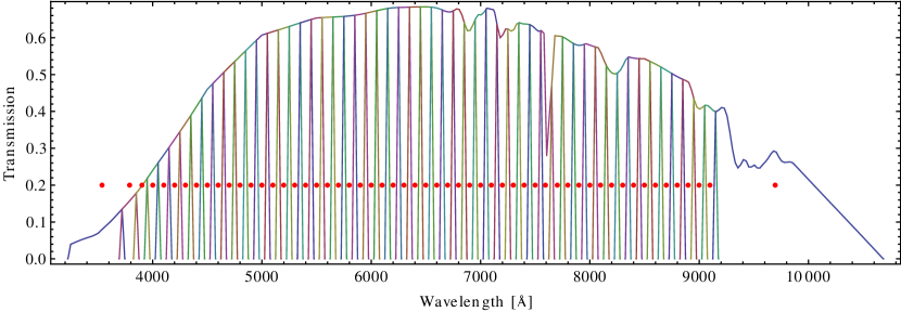
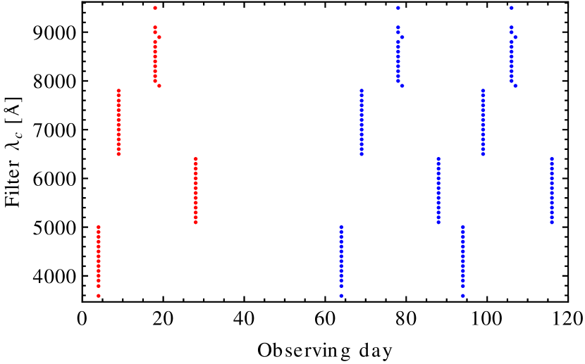
For this study we used the main contiguous J-PAS filters described in Fig. 2. These are 54 narrow band filters with width $\sim 145$ Å  and spaced by 100 Å, plus two broader filters at the ends of the wavelength range. For convenience, we will number them from 1 to 56 following their order in central wavelength $\lambda_{\mathrm{c}}$ (e.g. the bluest filter is number 1, the reddest filter is 56 and the reddest narrow band filter is 55). Each individual exposure, in each filter, will be of 60 s for filters 1–42 (3500 Å $\leq\lambda_{\mathrm{c}}\leq$ 7800 Å) and 120 s for filters 43–56 (7900 Å $\leq\lambda_{\mathrm{c}}\leq$ 9700 Å).

For simulating photometric data, other characteristics of the telescope, camera and site are necessary. We assumed an effective aperture of 223 cm, a plate scale of 22.67 $\mathrm{arcsec/mm}$ and a pixel size of 10 $\mathrm{\mu m}$. The CCD readout noise was set to 6 electrons per pixel, with a readout time of 12 s. These values are very close to the ones reported for J-PAS (Benitez et al., 2014). The point spread function was modelled as a Gaussian with dispersion $\sigma$ determined by a conservative estimate of the seeing (0.8 arcsec) at the J-PAS site (Observatorio Astrofísico de Javalambre, OAJ, Moles et al., 2010).

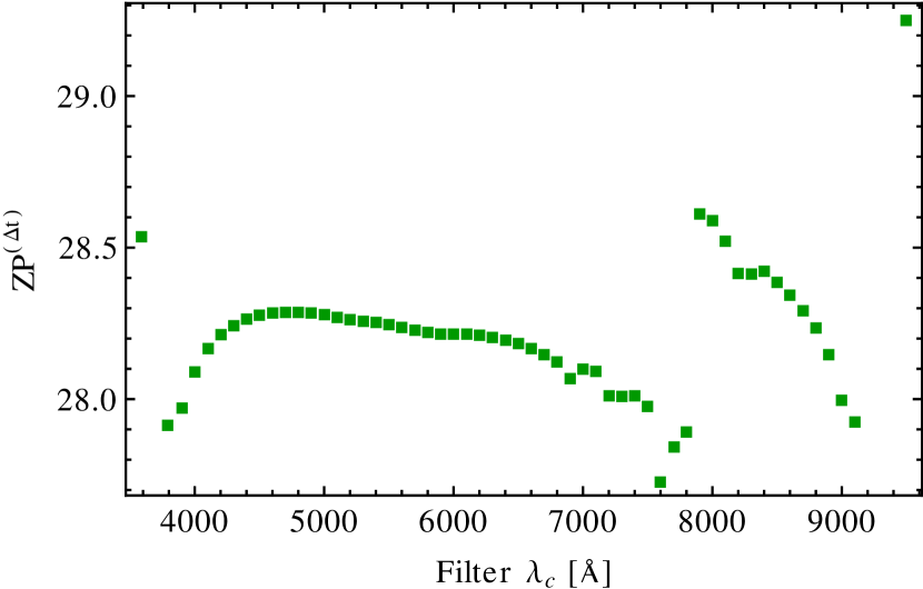
With this information, we can calculate the zero point that relates an object’s magnitude to its corresponding CCD electron count, an snana required input. Note that the zero points we refer to in this paper relate magnitudes to total counts instead of count rates as this is snana’s convention; to stress this fact we will call them $ZP^{\mathrm{(\Delta t)}}$. By assuming that the object’s spectrum is fairly constant within a filter wavelength range and using the AB magnitude system, we calculated the zero points $ZP_{n}^{\mathrm{(\Delta t)}}$ for the filter $n$ as:

$$ZP_{n}^{\mathrm{(\Delta t)}}=2.5\log_{10}\left[\frac{\pi D^{2}\Delta t_{n}}{4h}\int\frac{T_{n}(\lambda)}{\lambda}d\lambda\mathrm{\frac{erg}{cm^{2}}}\right]-48.6\;,$$ (6)

where $D$ is the telescope aperture, $h$ is the Planck’s constant, $\Delta t_{n}$ and $T_{n}(\lambda)$ are the filter $n$ exposure time and transmission function, respectively. Fig. 3 shows the average zero points used in the simulations.

When comparing narrow band to broad band surveys, more attention will be given to SDSS rather than DES since the former is much more similar to our fiducial survey: it also used a 2.5-m telescope with a field of view (FoV) of 7 $\mathrm{deg^{2}}$, and its exposure time was 55 s (Gunn et al., 2006; Frieman et al., 2008). In contrast, DES uses a 4-m telescope with a 3 $\mathrm{deg^{2}}$ FoV and an average exposure time of 230 s for its shallow fields (Bernstein et al., 2012).

Figure 3: Average zero points for the 56 filters. The large difference from filters 1 to 2 and 55 to 56 are due to their band size, and the difference between filters 42 and 43 (around 7900 Å) is due to the doubling in exposure time.

2.3 Survey strategy

Most astrophysical surveys have multiple goals and the final survey strategy may be a compromise between optimal strategies for different sciences. However, the SNe need for a particular observation schedule usually excludes them from the main parts of surveys. For instance, the SDSS supernova survey was restricted to the months of September through November, during the years 2005–2007, scanning a region of $\sim 300$ $\mathrm{deg^{2}}$ (Frieman et al., 2008). DES is expected to employ $\sim 32$ per cent of its total time and $\sim 10$ per cent of its photometric time for SN science, imaging an area of 30 $\mathrm{deg^{2}}$ (Bernstein et al., 2012). To test a possible optimisation of the survey’s time usage, we analysed a strategy suitable both for SN and for a galaxy survey at the same time. This multi-purpose strategy is termed 2+(1+1) and is likely to be adopted by J-PAS (although its particular implementation might not involve all its filters during the same observing season).

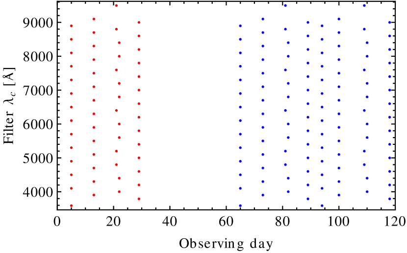
The 2+(1+1) strategy consists of a total of four exposures per filter per field. From the SN science perspective, the first two (which we call ‘template’) are used to form an image of the SN environment and are taken on the same night. If a SN shows up in the last two exposures (which we call ‘search’), the template is used to subtract the host galaxy. Therefore, it is important to leave a minimum time gap of approximately one month between the last template observation and the first search observation so the templates are not contaminated by the SNe. Fig. 4 presents a typical observation schedule for a given field.

In a real survey, the two template exposures would be combined into a deeper image; in this case, the errors on the two search exposures taken in the same filter would be correlated after the template subtraction, and this correlation would have to be taken into account during the data analysis. Unfortunately, snana was originally designed for surveys with very deep template images and does not fully support such analysis. To get around this issue we did not combine the two template exposures and used each one to subtract from a different search exposure. This approach trades the correlation between measurements for higher noise in each observation, thus making our simulations a conservative estimate of the capabilities of the survey.

During the search observations each field is imaged in 8 different epochs separated by $\sim 1$ week, and in each epoch the field is imaged using 14 different filters, making a total of 112 search observations (twice in each filter). The two exposures taken in the same filter are separated by $\sim 1$ month and it takes around two months to complete all search observations. In our main scenario schedule, the 14 filters that are observed in the same day are contiguous, which allows for the imaging of specific parts of the SN spectrum. Variations on this scenario are presented in section 4.

Figure 4: Example of observation schedule for our main scenario. The red and blue points represent the template and search observations, respectively. The filters being used in each day are identified by their central wavelengths $\lambda_{\mathrm{c}}$. Provided there is a gap of at least one month between template and search, the exact template schedule is irrelevant for SNe. Schedule realisations are affected by weather conditions and the SN angular position.

In our simulations, the SN observation schedule might be altered by the SN position in the field and by weather conditions which introduce a 0.16 chance of delaying a measurement. Moreover, complex particularities of the J-PAS filter positioning on the focal plane – whose specifications are beyond the scope of this paper – increase the survey’s footprint at expense of full filter coverage in some regions. In our fiducial SN survey, this translates into a 0.24 chance of 8 or more filters not being observed at all and into an effective FoV of 5.4 $\mathrm{deg^{2}}$. Assuming 8 hours of night time per day and the exposure and readout time from section 2.2, this strategy can be applied to $\sim 800$ $\mathrm{deg^{2}}$.

2.4 Host galaxy library

Our simulations made use of a library of host galaxies for two purposes: introducing extra Poisson noise left over after the host galaxy subtraction and for supplying a redshift prior when fitting the SN light curves. For each entry, the library contained the galaxy’s true redshift, its angular major and minor axis at half light (we used deVaucouleurs profiles), an orientation angle, the observed magnitude in each of the survey’s filters, and its photometric redshift (photo-$z$) and corresponding error. The orientation angle was drawn from an uniform distribution, while the luminosity profiles and magnitudes were drawn from actual SDSS data (Abazajian et al., 2009) for SN host galaxies (Gupta et al., 2011). To compute the magnitude of the host galaxies in the J-PAS filters we fitted SDSS DR5 spectral templates to SDSS broad band photometry and used the best-fitting spectrum to generate the narrow band fluxes.

The luminosity profile, the orientation angle and the observed magnitudes are only used to generate the extra Poisson noise in the SN photometry. A random galaxy at a similar redshift of the SN is chosen, along with the SN’s position on the galaxy, and then the flux coming from the galaxy is calculated. This flux is used to compute a CCD count which in turn serve as the mean value for a Poisson distribution from which the galaxy noise is drawn. Since the process of image subtraction increases the noise coming from the host galaxy (photon counts from the galaxy may vary between different exposures), we emulated this noise increase by making the galaxies brighter by a factor of $(1+1/N)$ [their magnitudes were decreased by $-2.5\log_{10}(1+\frac{1}{N})$, see Appendix A], where $N$ is the number of images of the galaxy alone, taken with the same exposure time as the SNe, that are combined into a single subtraction image. In our simulations, $N=1$. In any case, the host galaxy Poisson noise contribution proved to be sub-dominant when compared to other sources of errors (see section 3.1).

Although real galaxy photo-$z$s are usually non-Gaussian, we adopted Gaussian errors for simplicity. The photo-$z$s and corresponding errors adopted in our host galaxy library were based on J-PAS expected precision, which Benitez et al. (2009a, 2014) reported to be $0.003(1+z)$ for luminous red galaxies. Since not all galaxies may reach this error level we used a fixed precision of $0.005(1+z)$ for all SN hosts. This level of galaxy photo-$z$ accuracy is unique to narrow band surveys and, as shown is section 3.4, can also be attained from the SNe themselves.

2.5 Noise sources

The snana software includes many sources of noise to the simulated photometry: Poisson fluctuations from the source, the host galaxy and from the sky; CCD readout noise; a multiplicative flux error; and error on the Milky Way extinction correction. The multiplicative error on the flux (which can be translated into an additive error on the magnitudes) models a combination of errors such as standard stars measurement, flat fielding and other photometric technique errors (Smith et al., 2002; Astier et al., 2013; Kessler et al., 2013), and will be generically called calibration rms error $\sigma_{ZP}$. It is worth reminding that assuming a random error to model these effects is a simplification given that they might be correlated between different measurements. The CCD readout and the calibration rms errors were set to 6 electrons per pixel and 0.04 mag, respectively, for all filters, both conservative estimates. These and other relevant simulation parameters are summarised in Table 2. The effects of systematic uncertainties on the data are analysed in section 5.

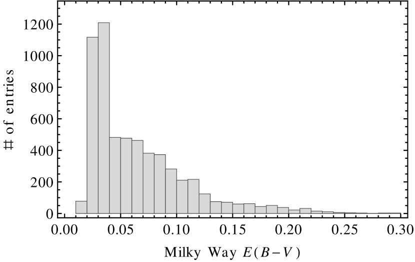
The Galactic extinction correction error used was the snana default (16 per cent). The true values of the excess colour $E(B-V)$ used for each SN simulation were drawn from a SDSS stripe 82 $E(B-V)$ sample presented in Fig. 5, and the extinction at each wavelength was calculated using the O’Donnell (1994) curve and $R_{V}=3.1$.

Figure 5: Histogram of the Milky Way excess colour $E(B-V)$ sample used to compute Galactic extinction on the SN fluxes.

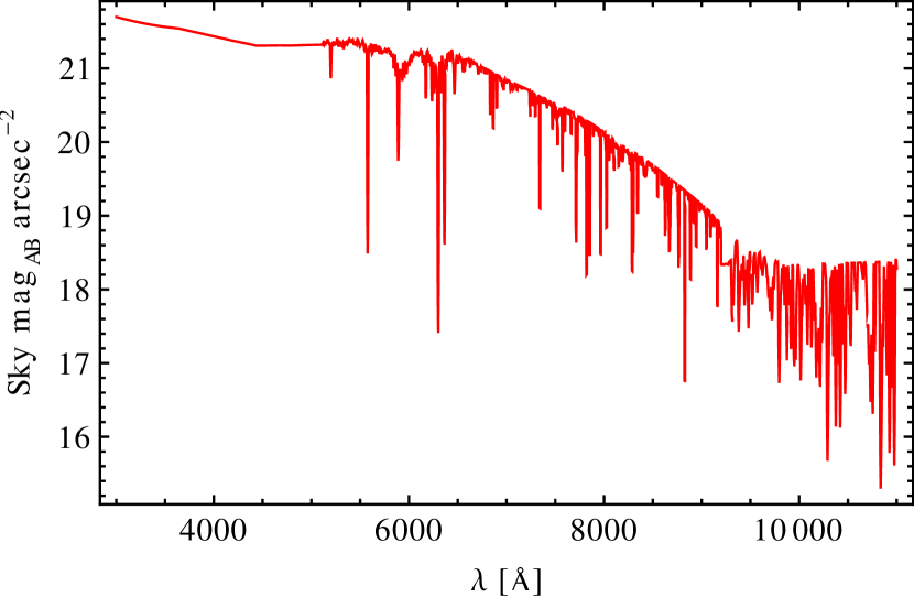
Based on an updated version of the sky spectrum from Benitez et al. (2009a), presented in Fig. 6, we estimated the photometry sky noise per pixel $\sigma_{\mathrm{sky},n}$ for filter $n$ using the following equation:

$$\sigma_{\mathrm{sky},n}^{2}=\frac{\pi D^{2}}{4}\Delta t_{n}P^{2}\int f_{\mathrm{sky},\lambda}(\lambda)T_{n}(\lambda)\frac{\lambda}{hc}d\lambda\;,$$ (7)

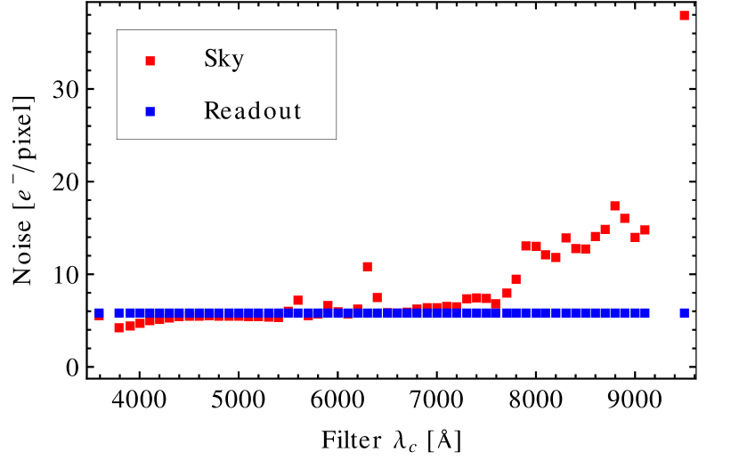
where $P$ is the pixel angular size in arcsec, $c$ is the speed of light and $f_{\mathrm{sky},\lambda}$ is the sky spectral energy density (SED) per $\mathrm{arcsec^{2}}$. Fig. 7 presents the obtained $\sigma_{\mathrm{sky},n}$ values and compare them with the CCD readout noise. Due to the narrow band nature of most filters, the adopted exposure time of 60 s makes the sky noise and the readout noise comparable.

Figure 6: Estimate of the average night sky spectrum for the J-PAS site, in AB magnitudes per $\mathrm{arcsec^{2}}$.

Figure 7: Estimated sky (solid red line) and readout (dashed blue line) noise per pixel for the 56 filters. Due to the small bandwidth of most filters, both noises are comparable.

The process of image subtraction required in SN surveys for removing the host galaxy flux increases the final SN photometry error. To account for this fact, we introduced this extra noise in the sky noise budget. The actual sky noise used in the simulations $\sigma^{\prime}_{\mathrm{sky},n}$ is related to the pure sky noise $\sigma_{\mathrm{sky},n}$ by:

$$\sigma^{\prime}_{\mathrm{sky},n}=\sqrt{\sigma_{\mathrm{sky},n}^{2}+\frac{1}{N}(\sigma_{\mathrm{sky},n}^{2}+\sigma_{\mathrm{r}}^{2})}\;,$$ (8)

where $N$ is the number of template observations combined into one subtraction image and $\sigma_{\mathrm{r}}$ is the readout noise per pixel.

Table 2: Observing characteristics assumed in our simulations: the telescope collecting area, the effective field of view, the CCD pixel size, its readout noise, the point spread function (PSF) radius and the rms uncertainty in the calibration.

Collecting area	39,507 $\mathrm{cm^{2}}$
Effective FoV	5.4 $\mathrm{deg^{2}}$
Pixel Size	0.228 arcsec	(10$\mathrm{\mu m}$)
Readout noise	6 $\mathrm{e^{-}/pixel}$
PSF $\sigma$	1.75 pixels	(0.4 arcsec)
Calib. rms error	0.04 mag

2.6 Data quality cuts

SN surveys usually impose various cuts on their data in order to ensure quality, and these cuts can be quite complex. Kessler et al. (2009a), for instance, required from the SDSS SNe at least: one measurement with signal-to-noise ratio (SNR) greater than 5 for each gri filter; five measurements at SN rest-frame epoch $t$ (measured in days from maximum luminosity) in the range $-15<t<60$; one measurement at $t<0$; one measurement at $t>10$; and a $\chi^{2}$ fitting probability for the MLCS2k2 light curve model (Jha et al., 2007) greater than 0.001. Unfortunately, given the big difference between the SDSS Supernova Survey and a narrow band survey, cuts cannot be transferred from one to the other, and therefore we must choose new cuts for selecting our simulated data.

A simple and effective quality cut is to require a minimum number of measurements with SNR greater than some threshold, regardless of the filter or the epoch. Since there is a high number of such observations (up to 112) and they are scattered along the epochs and wavelengths, this cut automatically requires that the SN is observed in many filters and in different epochs. Besides, more complex and optimised quality cuts are likely to be dependent on a specific survey strategy, which is not the goal of this paper. Thus, we classified the SNe according to the number of measurements with $\mathrm{SNR}>3$ that they possess and put them into samples called ‘Group 20’ (with a minimum of 20 such observations), ‘Group 30’ (with a minimum of 30 such observations) and so on. The number of measurements with $\mathrm{SNR}>3$ is highly correlated with the number of measurements with $\mathrm{SNR}>5$ but provides a smoother selection. The quality group 30 provides a good balance between sample size and data quality and will receive most of our attention.

2.7 SN typing and fitting process

The SN typing was performed with the psnid software (Sako et al., 2011) provided in the snana package. This software basically compares the SN photometric measurements to a grid of templates which includes variations of SN type (Ia, Ibc and II), sub-types and parameters. A $\chi^{2}$ is computed for each point in this grid and is used to calculate the Bayesian probability that an observed SN belongs to one of the three types – Ia, Ibc or II – by marginalising over their sub-variations in the grid. In the case of a SN Ia, these sub-variations correspond to variations in the SALT2 parameters. For CC-SNe, they correspond to variations in the redshift $z$, the distance modulus $\mu$, the host extinction at V band $A_{V}$, the ratio of total to selective extinction $R_{V}$, and to variations between different templates within that particular type. psnid uses four type Ibc and four type II SN templates created from Nugent et al. (2002) spectral templates, warped to match the photometry of eight spectroscopically typed nearby CC-SNe observed by SDSS. During the Bayesian probability calculations, psnid uses the host galaxy redshift and its associated uncertainty as the mean and the standard deviation of a Gaussian prior for $z$. The priors for the other parameters were assumed flat. More details about the psnid software can be found in Sako et al. (2011).

Our grid was built according to the ranges and intervals presented in Table 3. To classify a SN as type Ia, we required that its probability of belonging to this type should be above 0.9 (the sum of the three type probabilities is normalised to 1). Moreover, we required the $\chi^{2}$ $p$-value – calculated for the best-fit SALT2 model – to be greater than 0.01, so even if the type Ia model is the best fit for a light curve, it can still be ruled out as a bad fit. Given that psnid CC-SN templates are not fully representative of all our simulated CC-SN light curves, to classify a SN as core-collapse we only required a 0.10 probability of it belonging to any core-collapse template.

Table 3: Ranges and number of nodes for the grid used by psnid for typing SNe. Its parameters are the redshift $z$, the SN phase $t$ with respect to the time of maximum, a flux normalisation shift in mag $\Delta\mu$ from the value expected from fiducial cosmology, the SALT2 parameters $x_{1}$ and $c$, and the CC-SN host extinction parameters $A_{V}$ and $R_{V}$. All grid nodes are equally spaced with the exception of $z$ which is equally spaced in log scale.

Parameter	Min.	Max.	# nodes
$z$	0.01	0.70	160
$t$	-20	80	56
$\Delta\mu$	-2.0	2.0	41
$x_{1}$	-5.0	5.0	20
$c$	-0.4	0.4	6
$A_{V}$	-1.0	1.0	4
$R_{V}$	2.2	3.2	2

The fitting is performed by snana through a $\chi^{2}$ minimisation using the minuit software. All our SALT2 model fits were performed with four free parameters since the SN redshifts were fixed to their host’s photo-$z$s. In section 3.4, in particular, we perform a five free parameters fitting, leaving the SN redshift unconstrained.

The estimate of the distance modulus is performed by solving Eq. 5 for $\mu$. However, the so-called “nuisance parameters” $\alpha$, $\beta$ and $M$ are usually not fixed by local measurements and are determined from the same data by minimising the scatter around an average distance for a particular redshift. In our analysis, this process was performed using the salt2mu software (Marriner et al., 2011), which assumes a fiducial cosmology and uses different average absolute magnitudes $M_{i}$ for each redshift bin $i$ to account for possible discrepancies. The parameters $\alpha$ and $\beta$ are determined by minimising the scatter in these bins, while $M$ is defined as the weighted average of $M_{i}$.

2.8 Broad band survey simulations

The SDSS-II SN survey simulation was performed using the standard SDSS characteristics as implemented in the snana package and the same SN light curve models used for our narrow band simulations. Basically, the SDSS strategy consists of imaging the Stripe 82 region (300 $\mathrm{deg^{2}}$) in the ugriz filters every $\sim$ 4 days, on average. We also applied the default snana cuts required from the SDSS data:

1. at least three ugriz filters with one or more observations with $\mathrm{SNR}>5$, in any epoch;

2. at least one observation made before the SN luminosity peak;

3. at least one observation made after ten days from the SN luminosity peak;

4. at least five observations made in different epochs.

Two separate samples of simulated SDSS light curves were created, one associated with a redshift precision of 0.0005 (representing observations backed up by spectroscopy of the host galaxies) and another with a redshift precision of 0.03 (representing a pure broad band photometric survey). The first case was termed spec-$z$ SDSS and the second one photo-$z$ SDSS. As in our fiducial survey, all redshift errors were assumed to be Gaussian. We did not consider any selection effects or sample size reductions that might be caused by spectroscopic follow-up of host galaxies, and the sole difference between these two simulated broadband data is the redshifts assigned to the SNe. In practise, however, a spec-$z$ broadband survey is likely to have its sample sizes reduced due to the scarcity of spectroscopic time.

For comparing our narrow band survey outcomes with the DES SN survey we did not simulate DES light curves ourselves but used instead the results from Bernstein et al. (2012).

3 Results

The large area covered by our fiducial survey allows for a large number of SNe to be observed. Table 9 presents the number of SNe that could be added to a catalogue every two months of searching, for our various quality groups. As a reference we also present the values obtained for the SDSS-II SN Survey simulation.

Table 4: Number of SNe Ia and CC-SNe expected within each quality group, for every two months of search observations, assuming that the template observations have been made one month before them.  We only included SNe that passed light curve quality cuts and that were correctly typed. Results for an SDSS simulation were also included as a reference point.

Group	SDSS	20	30	50	70
# SNe Ia	330	760	500	210	75
# CC-SNe	60	120	90	50	25

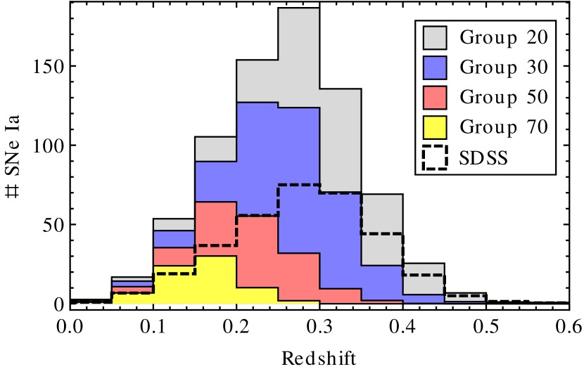
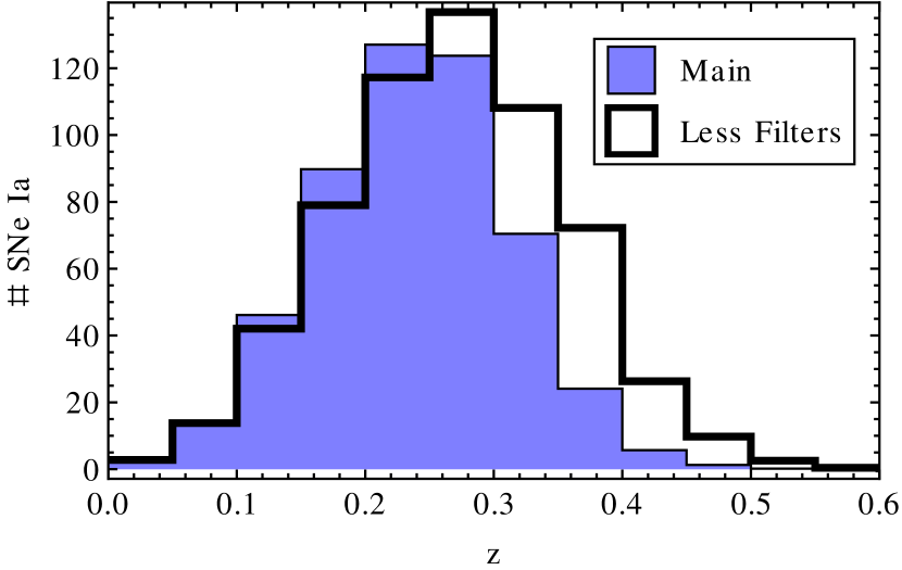
Fig. 8 shows the expected redshift distribution of correctly typed SNe Ia for our fiducial survey under various selection cuts and for the SDSS simulation as a reference. The distributions for quality groups 20 and 30 populate a slightly shallower interval than the one obtained for SDSS, whereas the total number of SNe Ia is much bigger due to the larger area covered. As shown by Bernstein et al. (2012), DES will use a 4-m telescope and longer exposure times to identify up to 4000 SNe Ia with a redshift distribution peaking at $z\sim 0.4$ and reaching $z\sim 1.2$. The DES SN survey will use about 1300 h of observing time (approximately 0.32 of the total survey time), making an average of 1500 SNe Ia every two months of dedicated SN survey time and 470 SNe Ia every two months of total survey time.

Fig. 8 also shows that an increase in the minimum number of observations with $\mathrm{SNR}>3$ required from the data reduces the sample sizes and redshift ranges. However, as presented in the following subsections, these reductions are accompanied by an increase in sample purity, photometry SNR and light-curve parameter recovery precision. An optimal balance can then be chosen according to the desired scientific goals.

Figure 8: SN Ia redshift distributions for our fiducial survey quality groups 20 (gray), 30 (blue), 50 (red) and 70 (yellow filling), superimposed in this order, from back to front. The number of SNe Ia was calculated for a season of two months of search imaging over 800 $\mathrm{deg^{2}}$. An increase in the minimum number of measurements with $\mathrm{SNR}>3$ decreases the average redshift and the number of SNe Ia that passes the cuts. Results obtained for the SDSS simulation (300 $\mathrm{deg^{2}}$), normalised to two months of search, are presented in thick, dashed contours (no filling).

3.1 Individual flux measurements

The change from broad to narrow band filters modifies the qualitative behaviour of the survey, for instance by changing the error budget. As presented in Fig. 7, the background noise from the sky is significantly reduced when compared to broad band, making the readout noise (often neglected in broad band imaging surveys) a relevant aspect of the survey. Moreover, since the calibration rms is a multiplicative flux error, it only contributes to the error budget at very low redshifts, while it might extend to higher redshifts for broadband surveys with the same exposure time.

Figure 9: Evolution of different error sources with redshift $z$, quantified by the CCD photon counting error (in photo-electrons, p.e.). The pink points represent the mean of the errors estimated by snana, and the curves are simplified analytic models representing: the quadratic sum of SN and host galaxy Poisson noise (green, dashed line, decreasing with $z$), the quadratic sum of the readout and sky noise in the PSF (blue, dashed line, constant in $z$); the calibration rms contribution (solid, thin red line) and the total error (solid, thick black line). The simplified model represents the simulated data well, the Poisson noise is sub-dominant and the calibration error dominates the noise up to $z\sim 0.1$

.

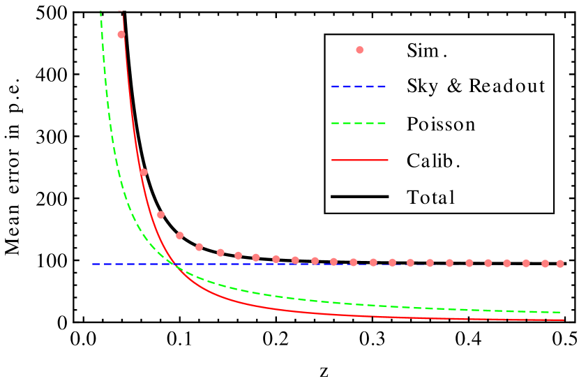
In Fig. 9 we compare the contributions from different error sources to the final flux measurement errors. The lines show simplified analytic error models which assume mean values for the zero point and for the sky noise and a fixed observer-frame absolute magnitude of -18.2 in all filters and redshifts. The points are the average of the results obtained from the detailed snana simulation. We can notice that the Poisson noise from the SN and the host galaxy is almost always sub-dominant; and that the calibration rms contribution dominates up to redshifts $z\sim 0.1$.

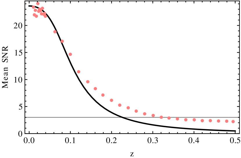
The small bandwidth of the filters also affects the SNR by lowering the signal (see Fig. 10). As expected, a narrow band survey will be shallower, maintaining a high SNR at lower redshifts. Selection effects are also expected to kick in a little before $z\sim 0.3$, when the average SNR reaches the level required (3 in this case) from some SN measurements. Due to the assumed calibration rms error of 0.04 mag, the SNR saturates, for low-$z$, at $\sim 25$.

Fig. 10 also shows the output from our simplified analytic model which is detailed in Appendix A (thick black line). It describes the general behaviour of the SNR reasonably well, although it underestimates the signal at higher redshifts. This is mainly due to effects that were ignored in our toy model: the drift with $z$ of the SN Ia luminosity peak from 4000 Å  to higher wavelengths (where the filter transmission is higher), an effect that can be accounted for with a K-correction; the time dilation of the light curves, that sustain detectable signals for longer periods; and selection effects such as the Malmquist bias.

Figure 10: Average SNR evolution with redshift $z$. The pink points represent the mean over simulated measurements with $\mathrm{SNR}>1$ for SNe Ia in group 30 (at least 30 observations with $\mathrm{SNR}>3$). Our photometry toy model is represented by the thick black line. The horizontal gray line indicates the SNR=3 level. The SNR saturates at $\sim 24$ for low-$z$ due to the multiplicative error $\sigma_{ZP}$, and at $\sim 3$ for $z>0.3$ due to our selection cuts.

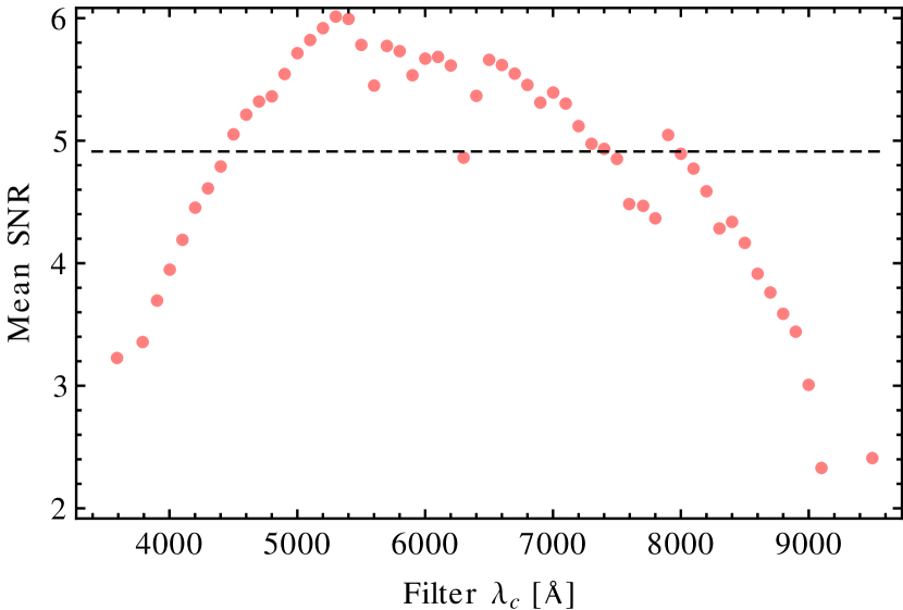
The results presented in Figs. 9 and 10 are an average for all filters, and the specific results vary within the filter set. In general, there are three aspects that alter a narrow band filter’s performance: its average transmission, the sky noise at its wavelength, and the SN Ia spectral energy density probed by the filter.

An increment in the average transmission increases the signal, thus basically stretching the SNR curve in Fig. 10 along the horizontal axis (the sky noise is increased a bit as well). This effect benefits the intermediate wavelength filters (4500–8000 Å, see Fig. 2). The sky noise will affect more strongly the reddest filters and those imaging the sky emission lines (see Fig. 6). Finally, filters probing dimmer parts of the SN spectrum will also present a stronger drop in SNR with redshift. Since our SN Ia model around the epoch of maximum luminosity is brighter at (rest-frame) $\sim 4000$ Å  and quickly drops for lower wavelengths, this will mainly affect the bluest filters, specially since the spectrum will be stretched to higher wavelengths for higher redshifts. The final result for the average SNR per filter is presented in Fig. 11. The toy model in Appendix A can be used to identify the effects of various survey characteristics on flux measurement errors and SNRs.

Figure 11: Average SNR per filter. The pink points present the mean over simulated measurements with $\mathrm{SNR}>1$ for SNe Ia in group 30 (at least 30 observations with $\mathrm{SNR}>3$).The dashed line indicates the average SNR for all filters. The effects of filter transmission functions, sky emission and different exposure times can be noted.

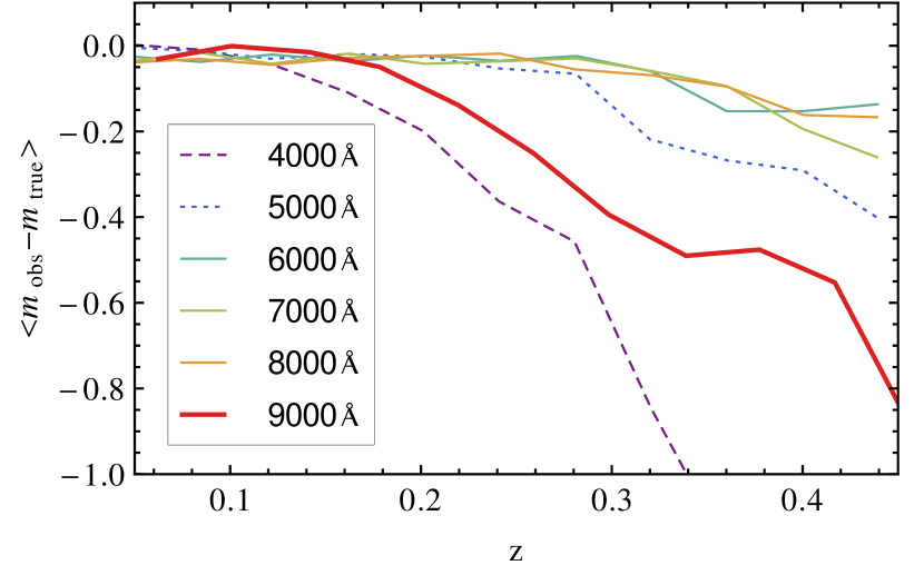
Another relevant effect present in each individual flux measurement is a form of statistical Malmquist bias: as photon counting at the CCD is a statistical process, measurements near the selection threshold with positive fluctuations tend to be detected while those with negative fluctuations do not. This leads to an overestimation of the average photon emission from the source which should be taken into account if one is interested in measuring spectral features and flux ratios, for instance. Fig. 12 shows this effect for six filters as a function of redshift, where we see that filters with lower average SNR (the very blue or very red) are the ones most affected. Apart from small fluctuations caused by the simulated sample finite size, the variations with redshift over the smooth dropping trend (better seen for the thick red curve) are caused by spectral features moving into and out of each filter’s band. Curves for filters not shown in the plot can be roughly estimated by interpolating the plotted ones.

Figure 12: Average difference between measured and true magnitudes for observations with $\mathrm{SNR}>1$ in filters numbers 4 (central wavelength $\lambda_{\mathrm{c}}=4000$ Å, dashed purple line), 14 ($\lambda_{\mathrm{c}}=5000$ Å, dotted blue line), 24 ($\lambda_{\mathrm{c}}=6000$ Å, thin cyan line), 34 ($\lambda_{\mathrm{c}}=7000$ Å, thin green line), 43 ($\lambda_{\mathrm{c}}=8000$ Å, thin orange line) and 54 ($\lambda_{\mathrm{c}}=9000$ Å, thick red line), as a function of redshift $z$. Filters on the outskirts of the wavelength range suffer stronger biases.

Figs. 13 and 14 compare observer frame SN Ia spectra near the epoch of maximum luminosity to simulated measurements. Both spectra and measurements include extinction by the Milky Way. To present a concise picture of the expected data quality we plotted the measurements on all 56 filters together in one epoch, but one should keep in mind that, in our fiducial strategy, the SN is observed in eight different epochs and in each one the observations are made on 14 contiguous filters (see Fig. 4).

Figure 13: Comparison between spectral template with Galactic extinction (orange line) and simulated measurements (data points) for a SN Ia at peak luminosity, at $z=0.157$, in the quality group 30. The average SNR for the plotted measurements is 12.1, and the spectrum units are arbitrary. Spectral features are clear. For brevity we show measurements on all filters, although in our fiducial strategy only a set of 14 different filters (presented as different markers and colours) would be observed on the same day.

Figure 14: Comparison between spectral template with Galactic extinction (orange line) and simulated measurements (data points) for a SN Ia 10 days after peak luminosity, at $z=0.33$, in the quality group 30. The average SNR for the plotted measurements is 4.9, and the spectrum units are arbitrary. Although noisy, large spectral features can still be detected. For brevity we show measurements on all filters, although in our fiducial strategy only a set of 14 filters (presented as different markers and colours) would be observed on the same day.

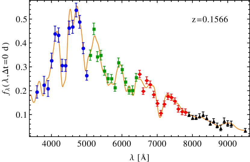
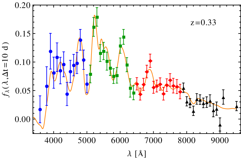
For low redshifts ($z<0.2$), the SN Ia spectral features are clear since they are much larger than the error bars (Fig. 13). In this redshift range, it is possible to detect and measure the light curves of nearly 170 SNe Ia every two months of search time (or every four months if the template imaging time is included). For higher redshifts ($z>0.3$), the measurements get noisier and this might prevent the detection of certain spectral features. However, as we show in section 3.3, global light-curve parameters – which are based on all 112 measurements – can still be measured to high accuracy.

3.2 SN typing

We calculated the contamination fraction $\eta_{\mathrm{Ia}}$ of an SN Ia sample by CC-SNe using the formula:

$$\eta_{\mathrm{Ia}}=\frac{W_{\mathrm{CC}}N_{\mathrm{CC}}}{W_{\mathrm{Ia}}N_{\mathrm{Ia}}+W_{\mathrm{CC}}N_{\mathrm{CC}}},$$ (9)

where $W_{X}$ is the fraction of SNe of type $X$ that was identified as Ia and $N_{X}$ is the expected number of type $X$ SNe per month of search. Table 5 shows that narrow band surveys can type SNe as well as broad band surveys, and that the performance is much higher for better quality groups. Estimates of SN Ia typing made by Bernstein et al. (2012) indicate that DES will reach completeness $W_{\mathrm{Ia}}$ of $\sim 0.85$ and contamination $\eta_{\mathrm{Ia}}$ around 0.02.

Table 5: Typing performance for SDSS SNe with host galaxy photo-$z$ and spec-$z$, and for various quality groups of our fiducial survey. The columns present, from left to right: the sample, the average number of observable SNe Ia and CC-SNe per month of search, the fraction of SNe Ia and CC-SNe identified as Ia, and the final Ia sample contamination by CC-SNe.

Sample	$N_{\mathrm{Ia}}$	$N_{\mathrm{CC}}$	$W_{\mathrm{Ia}}$	$W_{\mathrm{CC}}$	$\eta_{\mathrm{Ia}}$
photo-$z$ SDSS	172	46	0.96	0.214	0.0562
spec-$z$ SDSS	172	46	0.97	0.192	0.0503
Group 20	395	105	0.97	0.102	0.0274
Group 30	263	75	0.98	0.051	0.0148
Group 50	114	42	0.96	0.006	0.0023
Group 70	42	21	0.93	$\la 0.002$	$\la 0.001$

Table 5 also shows that the creation of an SN Ia sample is eased by the fact that its main sources of contamination – the CC-SNe – are dimmer than the SNe Ia (see Table 1) which reach absolute magnitudes of $M_{B}=-18.06$ or less (Phillips, 1993; Richardson et al., 2002). Thus, the CC-SNe populate lower redshifts, where the survey volume is smaller, and the number of detected CC-SNe is reduced. We can also see that photometric typing using broad bands can perform reasonably well, a result in agreement with other simulations (e.g. Campbell et al., 2013) and with real data analysis (Sako et al., 2011).

3.3 SALT2 parameter recovery

Another way of analysing the quality of the SN data obtainable by a narrow band survey is to verify its precision on the recovery of the light-curve parameters used to simulate the data. However, it is important to keep in mind that a narrow band survey offers many more possibilities than can be simulated here. For instance, in the SALT2 model the colour variation is simply an extinction law without any implications to the SN spectra, thus it can be precisely measured with broad band filters and no new information is gained with a better wavelength resolution. The $x_{1}$ simulation and recovery with SALT2, on the other hand, is better suited for a narrow band survey analysis as it reflects variations both on light-curve width and spectral features. Still, it is possible that some spectral variations not present in the simulations could be detected by narrow band filters. Thus, this analysis is to be understood as a coarse, general guide to the survey’s performance.

We selected all true SNe Ia that passed light curve cuts and were identified as Ias and binned them in redshift. For each SN we computed the difference $\Delta y=y_{\mathrm{f}}-y_{\mathrm{t}}$ between the fitted SALT2 parameter value $y_{\mathrm{f}}$ and the true one $y_{\mathrm{t}}$ ($y=m_{B},\;x_{1},\;c,\;t_{0}\;\mathrm{or}\;\mu$), and for each bin we computed the mean and the root mean square (rms) $\sigma_{y}$ of these differences. The mean can indicate the existence of any redshift dependent biases while the rms gives us a sense of the average error in each redshift bin. Their uncertainties were estimated as $\sigma_{y}/\sqrt{n}$ and $\sigma_{y}/\sqrt{2(n-1)}$, respectively, where $n$ is the number of SNe in that bin.

Figure 15: Bias (bottom points) and rms (top points) of the difference between recovered and true $m_{B}$ SALT2 parameter for our narrow band survey groups 30 (blue circles) and 50 (red squares). The gray bands on the top part of the plot represent a $\pm 2\sigma$ interval for the SDSS simulations rms and the bands on the bottom part represent $\pm 2\sigma$ interval for the SDSS simulations biases. The light bands represent the photo-$z$ SDSS and the dark bands represent the spec-$z$ SDSS. All surveys have similar rms and biases.

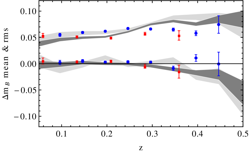
Fig. 15 shows the rms and bias calculated for the SN rest-frame apparent magnitude $m_{B}$ for our fiducial survey (quality groups 30 and 50) and for the SDSS simulations. All surveys suffer from a bias which overestimates the SN luminosity at higher redshifts (the difference $\Delta m_{B}$ between recovered and true $m_{B}$ tends to be more negative), although it is less perceptible for the narrow band survey simulations. This is a form of statistical Malmquist bias, as explained in section 3.1.

Figure 16: Bias (bottom points) and rms (top points) of the difference between recovered and true $x_{1}$ SALT2 parameter for our narrow band survey groups 30 (blue circles) and 50 (red squares). As explained in Fig. 15, the gray bands represent the results for the SDSS simulations. The narrow band survey have smaller errors, as do higher quality groups.

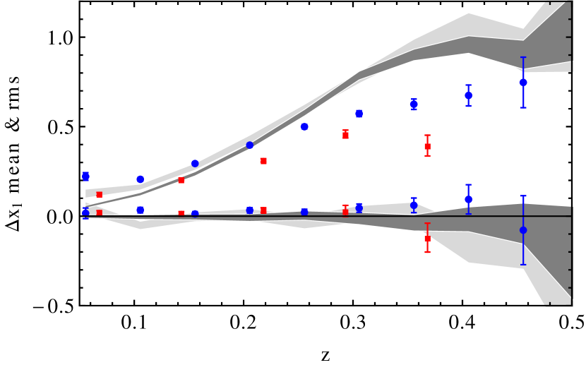
On Fig. 16 we notice that our fiducial survey can pin down more precisely the SALT2 $x_{1}$ parameter than our SDSS simulations, and that the increase in the data quality requirements also increases precision, as the $\Delta x_{1}$ rms is smaller for the quality group 50. The existence of a subtle constant bias favouring broader light curves (larger $x_{1}$) is possible, however this effect is very small – maybe reaching $\sim 5$ per cent of the rms – and is also insignificant for $\mu$ determination.

Figure 17: Bias (bottom points) and rms (top points) of the difference between recovered and true $c$ SALT2 parameter for our narrow band survey groups 30 (blue circles) and 50 (red squares). As explained in Fig. 15, the gray bands represent the results for the SDSS simulations. A strong redshift prior helps reducing the average errors, and broad band photometry is good at constraining $c$ as long as it is backed up with spectroscopic redshifts of the host galaxies.

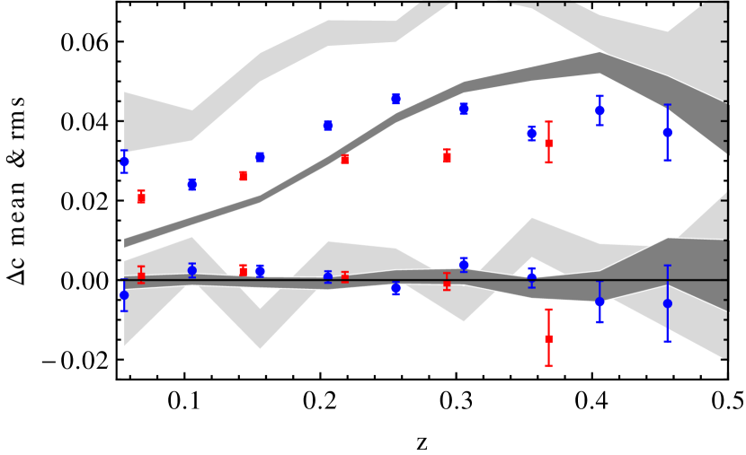
As suggested above, the advantages of narrow band filters are not as significant for constraining SALT2 colour $c$. Fig. 17 shows that spec-$z$ SDSS can perform as well as the narrow band quality group 30, on average, and better than both quality groups at low redshifts. DES, when backed up by spectroscopy, reach a colour rms of 0.031 in the range $0.2<z<0.4$ and an average of 0.046 for its full sample (Bernstein et al., 2012). It is also possible to notice that $c$ measurements are severely affected by a looser redshift prior, as shown by the photo-$z$ SDSS much larger rms. This is expected since a change in redshift drifts the SN spectrum and changes the expected flux in each observer-frame filter. Therefore, even if differences in colour are simply broad band features, pure narrow band surveys still yield better colour measurements than pure broad band surveys given their much better photo-$z$ constraints.

Figure 18: Bias (bottom points) and rms (top points) of the difference between recovered and true distance modulus $\mu$ for our narrow band survey groups 30 (blue circles) and 50 (red squares). As explained in Fig. 15, the gray bands represent the results for the SDSS simulations. All simulations suffers from biases and, apart from the photo-$z$ SDSS, all simulations are very close to the 0.14 intrinsic scatter.

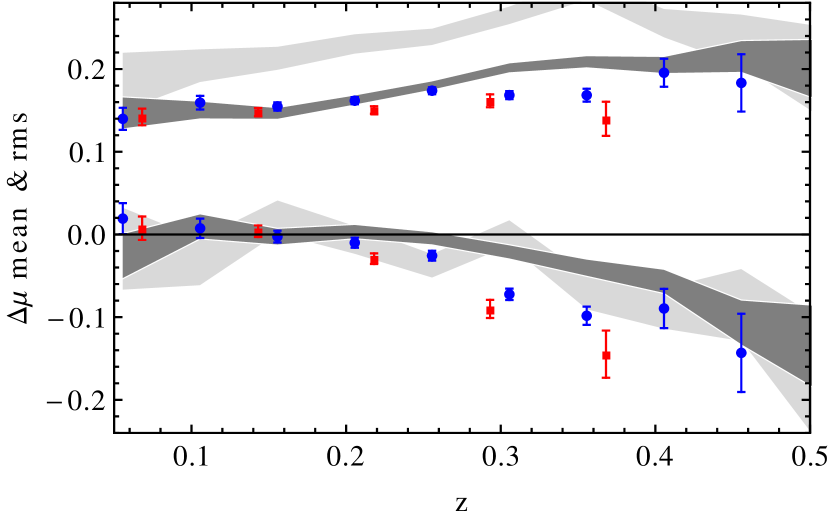
Finally, the quality of distance measurements with narrow band surveys is high, as its rms stays close to the SN Ia intrinsic scatter of 0.14 mag we assumed for our simulations (see Fig. 18). The DES simulations have $\sigma_{\mathrm{int}}=0.13$ and reached a $\Delta\mu$ rms of 0.16 in the range $0<z<0.5$ and an average of 0.20 for the full DES sample. It is also possible to see how the large uncertainty in $c$ caused by the loose redshift prior in the photo-$z$ SDSS simulation affects the distance measurements.

Fig. 18 also shows that all our simulations are affected by a bias that underestimates distances at large redshifts. This bias results from a combination of the $m_{B}$ bias presented in Fig. 15 and from a classical Malmquist bias of its own. The distance modulus $\mu$ is calculated from Eq. 5 by setting $m_{B}$, $x_{1}$ and $c$ to the measured values and $\alpha$, $\beta$ and $M$ to values that minimise the sample’s scatter around the distance predicted by a particular cosmology. However, this relation between $\mu$ and $m_{B}$, $x_{1}$ and $c$ is not perfect and this imperfection is modelled by the intrinsic scatter. Given that for fixed values of $\mu$, $x_{1}$ and $c$ the SNe Ia still present intrinsic luminosity variations, observations near the threshold will preferentially detect brighter objects, thus giving the impression of a smaller distance. For cosmological studies, this bias has to be corrected by simulations. Table 6 summarises the precision attainable in the SALT2 parameters by each SN Ia sample. We verified that the levels of CC-SNe contamination estimated in section 3.2 are too small to affect the determination of the nuisance parameters $\alpha$, $\beta$ and $M$ and, therefore, the distance inferred from SNe Ia.

Table 6: The rms of the differences between fitted and true SALT2 parameters. No binning in redshift was performed.

Group	$\sigma_{m_{B}}$	$\sigma_{x_{1}}$	$\sigma_{c}$	$\sigma_{t_{0}}$	$\sigma_{\mu}$
photo-$z$ SDSS	0.074	0.72	0.066	0.87	0.25
spec-$z$ SDSS	0.069	0.69	0.043	0.77	0.19
20	0.074	0.61	0.054	1.00	0.18
30	0.063	0.47	0.040	0.71	0.16
50	0.052	0.30	0.029	0.48	0.15
70	0.046	0.21	0.024	0.42	0.14

3.4 SNe photo-$z$ fitting

In our main analysis of SALT2 parameter recovery we fixed the SNe redshifts to their host galaxies photo-$z$s, and in the analysis of SN typing with psnid we used the host galaxies photo-$z$s as Gaussian redshift priors; in both cases, the errors on the host galaxies photo-$z$s were Gaussian with $\sigma_{z}=0.005$. In this section we briefly investigate the data outcome for SNe without including any information from their hosts. This translates into typing the SNe using a flat redshift prior and into doing a five-parameter instead of a four-parameter SALT2 fitting (the SN redshift is now a free parameter that can also be tested for recovery precision, and which we call “SN photo-$z$”).

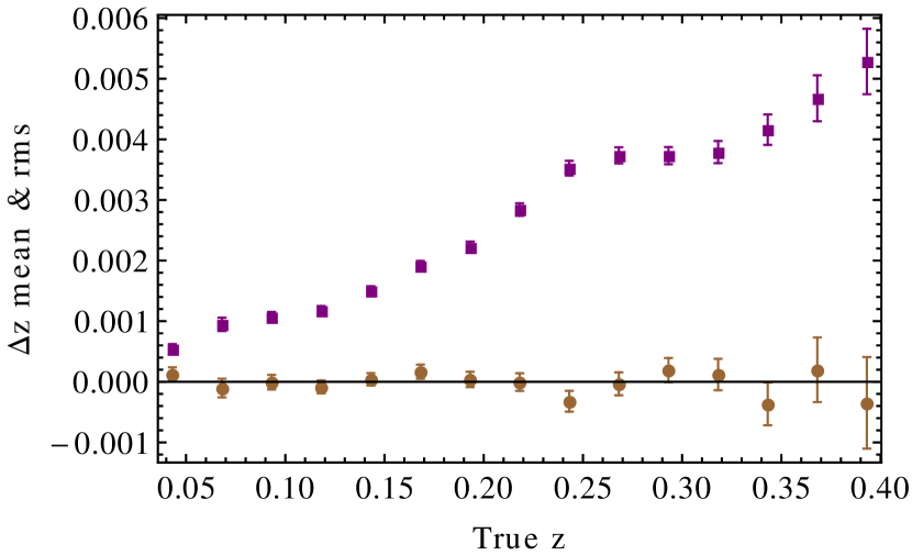
The SN photo-$z$ distribution obtained includes a small fraction of outliers (SNe with photo-$z$s more than 4$\sigma$ away from their true values), whose absolute difference between recovered and true redshifts commonly surpass 0.1. However, this fraction is very low, being 0.038 for the quality group 20 and reaching 0.007 for quality group 50. On top of that, the remaining SNe Ia have extremely accurate photo-$z$s, presenting a symmetrical error distribution, rms below 0.005 and no noticeable bias (Fig. 19 shows the SN photo-$z$ bias and rms for the quality group 30). This precision makes sense as narrow band filters can clearly detect SN spectral features (see Fig. 13 and 14). In comparison, Kessler et al. (2010a) and Sako et al. (2011) showed both with simulations and real data that SDSS SN photo-$z$ in the same redshift range is not free from bias and reach an average rms of $\sim 0.03$ or more. Notice that even though our simulations can reach very small photo-$z$ errors, in practise these are limited to 0.005 by intrinsic uncertainties such as the rms between SN and host galaxy redshifts (Kessler et al., 2009a).

Figure 19: Bias (bottom brown circles) and rms (top purple squares) of the difference between recovered and true redshifts for our narrow band survey quality group 30 when the SALT2 fitting is performed with the redshift as a free parameter and no host photo-$z$ information is used. In this plot we also removed outliers (SNe Ia with $\Delta z>4\sigma_{z}$, corresponding to $\sim$ 2 per cent of the sample). Our simulations can achieve very low rms and no significant bias for the majority of SNe Ia.

The use of the five-parameter SALT2 fit, however, introduces significant biases in all the other parameters: the SN Ia colour, for instance, was on average measured to be redder than in reality by 0.005 mag. A similar bias was already reported by Olmstead et al. (2013) for an analysis of SDSS SN data and was attributed to a bias in the SN photo-$z$ and its degeneracy with colour. To test if the SN photo-$z$ values are responsible for these biases we fixed them as the SN redshifts and reran the fitting, this time with four free parameters. All biases then disappeared, indicating that the five parameter fitting method might be responsible for them. This issue still needs further investigation.

Lastly, Table 7 shows that the lack of a Gaussian redshift prior made the narrow band typing performance slightly worse than before; however, it remained comparable to (or better than) those obtained for the SDSS simulations.

Table 7: Typing performance for our fiducial survey when a flat redshift prior is used instead of the Gaussian prior from the host photo-$z$. The columns are the same as in Table 5.

Sample	$N_{\mathrm{Ia}}$	$N_{\mathrm{CC}}$	$W_{\mathrm{Ia}}$	$W_{\mathrm{CC}}$	$\eta_{\mathrm{Ia}}$
photo-$z$ SDSS	172	46	0.96	0.214	0.0562
spec-$z$ SDSS	172	46	0.97	0.192	0.0503
Group 20	395	105	0.95	0.1519	0.0406
Group 30	263	75	0.97	0.0984	0.0284
Group 50	114	42	0.96	0.0152	0.0057
Group 70	42	21	0.96	0.0020	0.0010

4 Optimising the survey

In this section we look into possible ways of improving narrow band SN data, specially without requiring better instruments. It is clear that a larger light collecting area and lower noise levels will improve the data, even if in different ways. As exemplified by our photometry toy model presented in Appendix A, the effect of a larger mirror, better filter transmission, more exposure time and larger bandwidths are all the same in terms of increasing photometry SNR and redshift depth. A larger exposure time, however, results in a loss of sky area covered during an observing season (presenting a trade-off between SNR and number of SNe), while larger bandwidths result in a loss in spectral resolution. Both of these changes might be beneficial depending on the survey’s goals.

Although less noisy data are always better, noise reduction might result in bad trade-offs or might yield very little gain. As presented in Fig. 9, even though the calibration rms error dominates the error budget at low redshifts and limits the increase of the SNR, the number of SNe affected by it is small since the survey volume at low redshifts is small. Thus, to improve the SNR for a large number of SNe, we should pay attention to the signal and to the dominant noise sources at higher redshifts (sky and CCD readout).

Figure 20: Estimate of the average SNR at each redshift $z$ for our fiducial SN survey (black thick line), calculated with the toy model described in Appendix A. We compare it with a survey with improved calibration rms (25 per cent decrease in $\sigma_{ZP}$, dotted blue line), no readout noise ($\sigma_{\mathrm{r}}=0$, dashed gray line), and two times longer exposure times (solid red line). A lower multiplicative error $\sigma_{ZP}$ greatly improves data (but only at low-$z$) while decreasing CCD readout noise does not. More exposure time improves data at all redshifts.

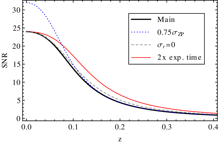
Fig. 20 compares the expected effects of improving calibration precision (in terms of reducing the zero point rms), decreasing the CCD readout noise and doubling the exposure time. A better calibration is highly beneficial for SNe at $z\la 0.1$, and such improvement might be worthwhile if one is interested in these objects (even though, as Fig. 8 points out, the amount of SNe Ia at $z<0.1$ is small). It is also possible to notice that the yield from reducing the readout noise is very small, even with an impossible $\sigma_{\mathrm{r}}=0$, as the sky noise is already comparable to $\sigma_{\mathrm{r}}=6\mathrm{e^{-}/pixel}$ (see Fig. 7) and would dominate the total noise at $z\ga 0.1$ if $\sigma_{\mathrm{r}}$ was reduced.

Fig. 20 also shows that increasing the exposure time would be beneficial to SNe at all redshifts. Keeping the total survey time constant, this increase can be achieved by reducing: (a) the area observed in one season; (b) the number of filters; (c) the cadence (number of times each field is observed in a given period of time); or (d) the so-called overhead time (time wasted, during observing hours, to read the CCDs and to reposition the telescope). Item (a) results in a simple trade-off with sample size and will not be further investigated here. Item (b) is analysed in section 4.2, while the effect of increasing the cadence [the reverse of item (c)] is studied in section 4.3. We investigate the effect of item (d) in section 4.4, and in the following subsection we present an optimisation method that does not involve increasing the SNR.

4.1 Dispersed observations

An interesting approach to improve SN data quality is to redistribute the observations among the epochs or the spectrum while maintaining the same SNR level for the individual flux measurements. Fig. 21 shows the observation schedule for this new scenario. In each epoch, the observations are evenly spread over the 56 filters set wavelength range. As in our main scenario (Fig. 4), only 14 filters are observed in each epoch, the search epochs are evenly distributed over $\sim 2$ months and each filter is observed in the 2+(1+1) strategy.

Figure 21: Example of observation schedule for our scenario with dispersed observations. The red and blue points represent the template and search observations, respectively (the template observations do not necessarily need to be dispersed). Four different sets of 14 filters are observed twice during template and twice during search observations. In each set, the filters are equally spaced in wavelength.

By repeating the analysis with this new observation schedule, our simulations show that our ability to constrain SALT2 parameters is significantly enhanced, specially for lower quality groups – which present more room for improvement. Colour is the most strongly improved parameter, probably due to the increased leverage of sampling the whole wavelength range in each epoch. Table 8 summarises the average SALT2 parameters uncertainties for this scenario and Fig. 22 compares, as an example, its $\Delta x_{1}$ rms redshift dependence for quality group 30 with the one obtained for the main scenario. The redshift distribution of the SNe Ia remained similar, as well as the bias on SALT2 parameters and on the distance modulus, although the subtle bias favouring larger $x_{1}$ got smaller in this scenario.

Table 8: The rms of the differences between fitted and true SALT2 parameters for the scenario with dispersed observations. No binning in redshift was performed.

Group	$\sigma_{m_{B}}$	$\sigma_{x_{1}}$	$\sigma_{c}$	$\sigma_{t_{0}}$	$\sigma_{\mu}$
photo-$z$ SDSS	0.074	0.72	0.066	0.87	0.25
spec-$z$ SDSS	0.069	0.69	0.043	0.77	0.19
20	0.061	0.50	0.039	0.88	0.17
30	0.054	0.39	0.032	0.63	0.16
50	0.046	0.27	0.023	0.44	0.15
70	0.044	0.18	0.017	0.32	0.15

Figure 22: Rms of the difference between recovered and true $x_{1}$ SALT2 parameter for quality groups 30 of the main scenario (black circles), the scenario with dispersed observations (green squares) and the scenario with less filters and more exposure time (cyan diamonds), as a function of redshift. Dispersed observations and more exposure time on fewer filters provide significantly better precision.

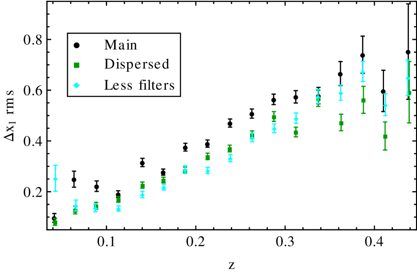
This improvement on constraining light-curve parameters is easy to understand if we remember that we are trying to constrain a spectral surface $f_{\lambda}(\lambda_{\mathrm{obs}},t_{\mathrm{obs}})$ (Eq. 1): if our measurements are better spread over this surface, we have a better idea of its shape (see Fig. 23 for a helpful representation of this idea). It is true that some regions of the spectra might vary more and thus contain more information, but these region’s location change with redshift. Therefore, an even sampling of $f_{\lambda}(\lambda_{\mathrm{obs}},t_{\mathrm{obs}})$ might be the best option for constraining its parameters. It is important to remember that although this strategy is better for describing overall characteristics of the light curves, one looses information about specific spectral features that might be measured within our main scenario.

Figure 23: SN Ia spectral surface $f_{\lambda}(\lambda_{\mathrm{obs}},t_{\mathrm{obs}})$ at $z=0.25$, convolved with a top-hat function 100 Å  wide, in arbitrary flux units. The time $t_{\mathrm{obs}}$ axis is given in days from maximum luminosity. The red points depict measurements in 54 narrow band filters following the strategy with dispersed observations (errors not included). A good sampling of $f_{\lambda}(\lambda_{\mathrm{obs}},t_{\mathrm{obs}})$ can better constrain its parameters.

4.2 Less filters, more time

By analysing SN spectra, one notices that the most luminous parts and many important features for typing SNe (H, He and SiII lines) lie below $\sim 6400$ Å  and only enter the reddest filters ($\lambda\ga 8000$Å) at redshifts $z\ga 0.25$, when our SN Ia redshift distribution starts declining. Therefore, for our survey’s depth, these filters convey little information about supernovae, and their allocated time might be put to better use if distributed among the other filters.

We created a new scenario in which the reddest 14 filters (which, in our main scenario, had twice the regular exposure time – see section 2.2) were removed and their time evenly distributed to the other filters. This filter removal also saved overhead time, and we were able to increase the remaining filter’s exposure time by 73 per cent.

When comparing this scenario with our main scenario, it is important to keep in mind that the same requirements in terms of number of observations with $\mathrm{SNR>3}$ result in a more restrictive selection for the scenario with less filters since the chance of achieving a certain number of good observations is smaller when the total number of observations is smaller. Thus, the best way of comparing the results is to remember the trade-off between number of SNe and data quality and take both into account.

Figure 24: SN Ia redshift distribution for the main scenario (thin contours, blue filling) and for the scenario with less filters (thick contours, no filling). Both histograms are for two months of search observations and quality group 30. The decrease in the number of filters and the corresponding extension of exposure time increased the survey’s depth and the total number of SNe Ia from 500 to 610 every two months of search.

As expected, the increase in exposure time made the survey more deep and massive (see Fig. 24). Table 9 also shows that the precision in the recovery of SALT2 parameters improved for $x_{1}$, $c$ and $m_{B}$, whereas it got slightly worse for $t_{0}$ – probably due to the smaller number of observing epochs – and remained practically the same for $\mu$ since it is limited by the intrinsic scatter. As an example, Fig. 22 shows the redshift dependence of the $\Delta x_{1}$ rms for this scenario. The typing performance remained basically the same.

Table 9: The rms of the differences between fitted and true SALT2 parameters for the scenario without the 14 reddest filters. No binning in redshift was performed.

Group	$\sigma_{m_{B}}$	$\sigma_{x_{1}}$	$\sigma_{c}$	$\sigma_{t_{0}}$	$\sigma_{\mu}$
photo-$z$ SDSS	0.074	0.72	0.066	0.87	0.25
spec-$z$ SDSS	0.069	0.69	0.043	0.77	0.19
20	0.064	0.58	0.056	1.00	0.20
30	0.057	0.43	0.037	0.78	0.17
50	0.051	0.27	0.024	0.53	0.16
70	0.046	0.16	0.017	0.39	0.14

4.3 Less SNR, more cadence

Due to the transient nature of SNe, a higher spectral surface sampling rate in time yields better constraints to its shape. For a fixed instrument, this increase in cadence is achieved by saving observing time either by reducing the area imaged or by reducing the time spent in each individual exposure. Whereas the first option clearly results in a trade-off between number of SNe observed and light curve measurement quality, in principle it is not obvious what the effect of the second option would be: while each individual measurement would have a smaller SNR, the amount of independent measurements would be higher.

To test this last option, we simulated SN observations where each filter was imaged four times instead of two, while the individual exposure times were reduced from 60 to 23.9 s for filters number 1–42 and from 120 to 53.9 s for filters number 43–56. These exposure times were chosen so as to keep constant the observed area of the sky (note that the increase in the number of exposures also increases the amount of wasted overhead time).

In terms of typing efficiency and recovery of SALT2 parameters, this simulation presented basically the same performance as our fiducial strategy, indicating that a larger number of observations can compensate for a smaller individual SNR, at least in the range tested. However, the SNR reduction decreases the survey depth, thus making the overall performance worse for this scenario.

4.4 Overhead time reduction

Assuming that the overhead time $t_{\mathrm{o}}$ is dominated by CCD readout time $t_{\mathrm{r}}$, one can trade low $\sigma_{\mathrm{r}}$ and high $t_{\mathrm{o}}$ for high $\sigma_{\mathrm{r}}$ and low $t_{\mathrm{o}}$ since $\sigma_{\mathrm{r}}$ and $t_{\mathrm{r}}$ follow a power-law relation:

$$\sigma_{\mathrm{r}}=\left(2+\frac{50\mathrm{s}}{t_{\mathrm{r}}}\right)\mathrm{e^{-}/pixel}.$$ (10)

The relation above was based on Jorden et al. (2012) and adjusted to match $\sigma_{\mathrm{r}}(t_{\mathrm{r}}=12\mathrm{s})=6\mathrm{e^{-}/pixel}$. The time saved from reading the CCD could then be used to increase the exposure time and therefore the flux signal. This potential option for improving the SNR was investigated only through the use of our photometry toy model.

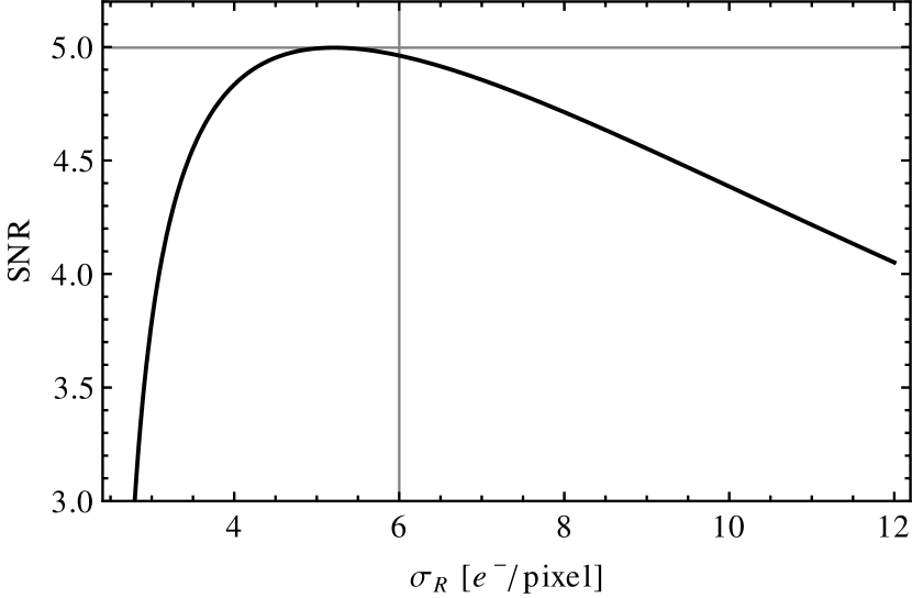
Fig. 25 shows how the average SNR responds to such trade, assuming that the time saved from CCD reading is used to increase exposure time. Although it is beneficial to increase $\sigma_{\mathrm{r}}$ in some regimes, our fiducial value is close to the optimum and not much can be gained from this trade.

Figure 25: Average SNR for a SN Ia at $z=0.19$, calculated for a narrow band survey using the toy model from Appendix A, as a function of the CCD readout noise, assuming that observing hours are fixed and split between exposure time and CCD readout time and that readout noise and time follow the relation presented by Eq. 10. Vertical and horizontal gray lines are shown as references. The relations for different redshifts are very similar.

5 Systematic uncertainties

Our choice of systematic uncertainty sources to be studied was based on the list presented by Bernstein et al. (2012) for the DES supernova simulations: (a) offsets on the filter zero points; (b) offsets on the filter central wavelengths; (c) contamination by CC-SNe; (d) an error on the priors adopted for dust extinction; and (e) bias on inter-calibration with low redshift SN Ia samples. However, many of these sources are not intrinsic to the instrument and filters used: item (d) only applies to the MLCS2k2 model and item (e) involves the combination with other data sets. The contamination by CC-SNe (c) might depend on the instrument and strategy as it depends on selection effects, however it impacts specific uses of SN Ia samples – like measuring the equation of state of dark energy – and not the individual measurements or the recovery of SALT2 parameters. Moreover, Bernstein et al. (2012) showed that the systematic uncertainty caused by a contamination level similar to ours was sub-dominant, so we focused our analysis on the effects of offsets (a) on the filter zero points and (b) on the filter central wavelengths. We also analysed the effects of biases in the photo-$z$ in section 5.3 as they may be relevant for our particular survey.

5.1 Filter central wavelengths

In practise, the filter set used to image the SNe will not be exactly like the synthetic transmission curves we use to compute the expected fluxes from the SALT2 model, and this mismatch will introduce systematic errors on the measurements. To estimate these errors we created a new filter set by applying a random offset to the central wavelength $\lambda_{\mathrm{c}}$ of each filter. This offset was drawn from a uniform distribution limited to $\pm 2.5\times 10^{-3}\lambda_{\mathrm{c}}$, which is a conservative specification for the J-PAS filters (Marin-Franch et al., 2012).

The SN fluxes were simulated with this new set of filters, and the simulated measurements were fitted both with our fiducial filter set (thus introducing the mismatch between assumed and actual filters) and with the same set used to simulate the data (which served as a systematics–free reference). The best-fitting SALT2 parameters under the two filter sets were compared for each individual SN Ia.

The mismatch between the true and assumed central wavelengths introduces a redshift dependent bias to the SALT2 parameters which frequently presents oscillations, specially for $c$, $m_{B}$ and $\mu$, while $t_{0}$ is the least affected parameter. These oscillations have a period within the range $0.08\la\Delta z\la 0.14$, while their amplitude depends on the average offset applied and their phase does not follow any clear relation. Fig. 26 shows an example of this bias for the colour parameter.

Figure 26: Average difference between the recovered values for the SALT2 colour parameter when the SNe Ia are fitted using mismatched and correct filter sets, as a function of redshift. The use of a synthetic filter set with wrong central wavelengths introduces a small oscillatory bias to the measured SALT2 parameters.

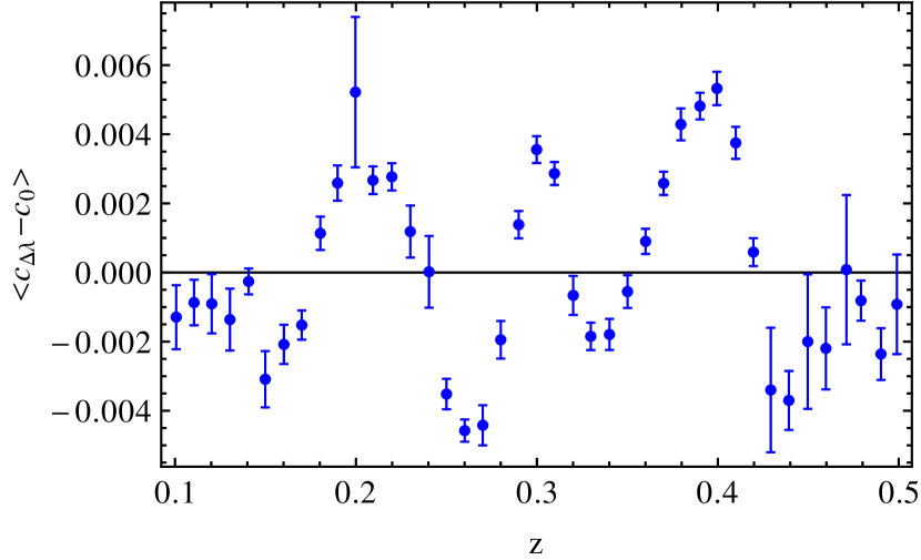
The oscillatory characteristic of the bias might be explained by the series of peaks and troughs in the SN Ia spectrum that, at its peak luminosity, repeat itself approximately every 500 Å. To understand how these two could be tied, imagine that a certain blue filter has an assumed central wavelength $\lambda_{0}$ and a true central wavelength $\lambda_{\Delta}$, shifted to a smaller value. At a certain redshift $z_{1}$, $\lambda_{0}$ coincide with a spectral peak while $\lambda_{\Delta}$ do not. Therefore, we will measure a flux smaller than expected for $\lambda_{0}$ and conclude that the SN is redder than in reality. For a SN Ia at a higher redshift $z_{2}$, when $\lambda_{0}$ coincides with a spectral trough, the measured flux will be higher than expected for $\lambda_{0}$ and we will conclude that the SN is bluer. The cycle repeats at a higher redshift $z_{3}=z_{1}+\Delta z$ when another peak appears at $\lambda_{0}$. While the exact $\Delta z$ needed to make two consecutive peaks appear in the same filter depends on $z_{1}$ and $\lambda_{0}$, it amounts to $\sim 0.12$ for the average filter and redshift.

In a real survey the filter central wavelength would vary across the field, different observations for each SNe would be dithered and each SNe would be observed in different regions of the filter. On one hand this eliminates part of the systematic error as statistical error, which in turn gets overwhelmed by the other error sources; this makes our estimates for this systematic uncertainty more conservative. On the other hand, the inhomogeneity of the filters and the dithering technique result in the galaxy subtraction being performed at slightly different wavelengths, a potentially harmful effect, specially if sharp galaxy spectral features are included or excluded by the wavelength shift. This might introduce strong random fluctuations in the photometry that are not represented by the error estimates. Such effect cannot be modelled in snana and will not be analysed here, but it should be investigated in the future.

Table 10: Estimated systematic errors on the SALT2 parameters caused by shifts on the filter central wavelengths, each randomly drawn from a uniform distribution within the range $\pm 0.25\%$ and $\pm 0.08\%$ of the filter’s central wavelength.

$\Delta\lambda_{\mathrm{c}}$ range	$\sigma_{m_{B}}^{\mathrm{sys}}$	$\sigma_{x_{1}}^{\mathrm{sys}}$	$\sigma_{c}^{\mathrm{sys}}$	$\sigma_{t_{0}}^{\mathrm{sys}}$	$\sigma_{\mu}^{\mathrm{sys}}$
$\pm 0.25\%$	0.0053	0.041	0.0034	0.047	0.0070
$\pm 0.08\%$	0.0015	0.014	0.0010	0.013	0.0021

The resulting $1\sigma$ systematic errors caused by the mismatch between assumed and real filter wavelengths are shown in Table 10. We also present the estimated errors for offsets between $\pm 0.8\times 10^{-3}\lambda_{\mathrm{c}}$, roughly the precision one would get by characterising the filters with a spectrophotometer and using the measured transmission curves as the synthetic ones. Lastly, we remark that mismatched filters could also introduce biases in the host galaxy photo-$z$s which in turn could impact the SN parameter measurements. Unfortunately, the effect of mismatched filters on the galaxy photo-$z$ is beyond the scope of this paper, although we verified that their effect on the SN photo-$z$s leads to systematic uncertainties of 0.001 and 0.0004 for offsets between $\pm 2.5\times 10^{-3}\lambda_{\mathrm{c}}$ and $\pm 0.8\times 10^{-3}\lambda_{\mathrm{c}}$, respectively, which are much less than the photo-$z$ rms errors of 0.005. We also verified the impact of constant photo-$z$ biases in SN Ia parameters in section 5.3. We emphasise that for J-PAS, in particular, filters will be fully characterised so that the central wavelength offsets will be smaller than $\pm 0.8\times 10^{-3}\lambda_{\mathrm{c}}$. Moreover, the galaxy photo-$z$s will be computed from a stack of dithered images, further reducing the average offset and its influence to negligible levels.

5.2 Calibration biases

To test the effects of photometry calibration biases on the SN data we applied random offsets to each filter zero point, drawing from a Gaussian distribution with standard deviation $\sigma_{\mathrm{\Delta ZP}}=0.01$, the same precision expected for DES (Bernstein et al., 2012). The application of a zero point recalibration technique based on photometric redshift estimations from emission line galaxies (Molino et al., 2014) might make this level of bias a conservative estimate. We adopted random offsets as a simplifying assumption since the specification of more complex biases would require detailed analysis of calibration methods which is beyond the scope of this paper.

As with shifts on the filter central wavelengths, the resulting SALT2 parameter biases from zero point offsets are usually redshift dependent. However, no clear common pattern could be identified: various realisations of the bias may lead to different general trends, offsets and fast variations on SALT2 parameters. Table 11 presents the average difference between SN Ia fits with and without the calibration bias. Their values are of the same order of the $\pm 0.8\times 10^{-3}\lambda_{\mathrm{c}}$ shift on the filter central wavelengths presented in section 5.1. The systematic uncertainty on the SN photo-$z$ resulting from this calibration bias was 0.0004, also comparable to the $\pm 0.8\times 10^{-3}\lambda_{\mathrm{c}}$ offset uncertainty.

Table 11: Estimated systematic errors on the SALT2 parameters caused by offsets on the filter zero points, each randomly drawn from a Gaussian distribution with $\sigma_{\mathrm{\Delta ZP}}=0.01$.

$\sigma_{\mathrm{\Delta ZP}}$	$\sigma_{m_{B}}^{\mathrm{sys}}$	$\sigma_{x_{1}}^{\mathrm{sys}}$	$\sigma_{c}^{\mathrm{sys}}$	$\sigma_{t_{0}}^{\mathrm{sys}}$	$\sigma_{\mu}^{\mathrm{sys}}$
0.01	0.0019	0.014	0.0012	0.015	0.0024

5.3 Photo-$z$ biases

Typical systematic galaxy photo-$z$ biases are about 0.33 of the rms error, and using spectroscopy to calibrate the photo-$z$s might help reducing it. To test the effects of such bias on SN Ia data we created four different simulations, each one with a constant offset on the host galaxy photo-$z$s: $\pm 0.001(1+z)$ and $\pm 0.002(1+z)$.

The average effect of a photo-$z$ bias on SN colour is simple: if the redshift estimate is higher than its true value, the SN image will seem bluer than expected for that redshift and the inferred colour will be smaller than its true value. If the redshift estimate is lower than the true value, the SN will seem redder. On the other hand, the effect on the $x_{1}$ estimate is more complex since two distinct redshift dependent effects compete: light curve time dilation and spectral shift in wavelength. Given that light curves are stretched by redshift (time intervals are longer at higher redshifts – see Eq. 1), assuming a smaller redshift for the SN will lead to a larger $x_{1}$ estimate since it will have to compensate for the unaccounted extra bit of time dilation. In opposition, light curves on the bluer part of the SN spectrum are usually narrower than redder light curves (see Fig 23). Therefore, a smaller redshift estimate will make one take a bluer light curve for a red one, pushing the $x_{1}$ estimate to smaller values. The resulting $x_{1}$ bias from these two effects depends on the redshift and filter set, and in our particular case, the spectral shift effect seems to be slightly larger for $z\la 0.3$ while time dilation dominates at $z\ga 0.3$.

The apparent magnitude $m_{B}$ is also affected by competing effects: at lower redshifts, the SN spectrum is more compact in wavelength space (there would be more photons per unit wavelength), so underestimations of $z$ make the SN look fainter. However, the SN rest-frame spectrum peaks at $\sim 4000$ Å  – almost outside our filter set wavelength range – so underestimations of $z$ leads to the wrong conclusion that one is measuring fainter regions of the SN spectrum, therefore increasing the inferred luminosity.

Finally, the distance modulus $\mu$ is affected by the biases in $m_{B}$, $x_{1}$ and $c$ and by a combination of Malmquist bias and misguided estimates of the nuisance parameters $\alpha$ and $\beta$: at higher redshifts, our survey preferentially detects more luminous SNe Ia, which would lead to underestimations of the luminosity distance. Since these SNe tend to be bluer, the term $-\beta c$ in Eq. 5 partially corrects for this effect. However, the biases in $x_{1}$ and $c$ induce slightly off $\alpha$ and $\beta$ values which will under or over-correct distance measurements. We remind that all the processes presented here describe average effects on SNe Ia data. The effects of a photo-$z$ bias on each individual SN is much harder to predict or describe. Table 12 presents the estimates for the systematic errors on SALT2 parameters due to photo-$z$ biases of order $0.001(1+z)$ and $0.002(1+z)$.

Table 12: Estimated systematic errors on the SALT2 parameters caused by $0.001(1+z)$ and $0.002(1+z)$ systematic biases in the photo-$z$s.

$\Delta z/(1+z)$	$\sigma_{m_{B}}^{\mathrm{sys}}$	$\sigma_{x_{1}}^{\mathrm{sys}}$	$\sigma_{c}^{\mathrm{sys}}$	$\sigma_{t_{0}}^{\mathrm{sys}}$	$\sigma_{\mu}^{\mathrm{sys}}$
$\pm 0.002$	0.0040	0.031	0.0037	0.062	0.0096
$\pm 0.001$	0.0018	0.012	0.0019	0.031	0.0059

In case of a photo-$z$ bias in which the offsets $\Delta z_{i}$ applied to each SN $i$ have $\langle\Delta z_{i}\rangle\neq 0$ (such as the constant bias we simulated), $\mu$ will get an extra constant offset, roughly of order $\mu_{0}(\bar{z}+\langle\Delta z_{i}\rangle)-\mu_{0}(\bar{z})$, due to a bias on the nuisance parameter $M$. Here, $\mu_{0}$ is the fiducial distance modulus used to estimate the nuisance parameters (see section 2.7) and $\bar{z}$ is the average redshift of the survey. Since constant offsets in $\mu$ are irrelevant for many applications, these are not included in Table 12.

6 Summary and conclusions

We used the snana software package and the SALT2 model to simulate the SN Ia data that a narrow band survey could obtain. We adopted J-PAS as our survey model, which is going to image 8500 $\mathrm{deg^{2}}$ of the sky in 54 narrow band ($\sim 100$ Å) and five broad band filters (see Fig. 2 for the transmission curves of the unique filters) and that can reach a galaxy photo-$z$ precision of $0.005(1+z)$ (Benitez et al., 2014). The observing strategy we assumed is called 2+(1+1). Each field would be imaged four times in each one of the 56 filters: twice during the same night in order to measure the flux from host galaxies and twice in different nights (spaced by $\sim$ one month) in order to find SNe and measure their light curves. In each night, 14 different filters are imaged, and the gap between different sets of filters is $\sim$ one week (Fig. 4 shows a graphical representation of this observation schedule).

First, we showed in section 3 that such an SN survey is indeed possible and can yield precise measurements of spectral features (see Figs. 13 and 14), light-curve parameters (Figs. 15–18 and Table 6), SN photo-$z$s (Fig. 19) and can achieve low contamination fractions by CC-SNe (see Table 5), all without any spectroscopic follow-up. This might be surprising since each light curve only has two measurement points. To understand this result, one should bear in mind that there are 56 light curves (making a total of 112 observations) and they all are being described by the same 5 parameters. This is even clearer if one thinks in terms of constraining a spectral surface $f_{\lambda}(\lambda_{\mathrm{obs}},t_{\mathrm{obs}})$ instead of light curves (see Fig. 23). We also studied potential systematics (section 5) – with photo-$z$ biases being the most relevant ones – and showed that they are small (less than 0.10 of the rms). The systematic uncertainties on the SNe Ia parameters are also more than 10 times smaller than known differences between SNe Ia in different environments (e.g. Xavier et al., 2013), so our fiducial survey still has room for the discovery of smaller, unknown potential differences.

On top of the precision attainable, a telescope with a large field of view may lead to massive samples (approximately 500 SNe Ia and 90 CC-SNe every two months – see Table 9) that can be used in the study of rates, spectral feature relations, dust extinction and intrinsic colour variations and correlations between SN and environment properties. Besides the increase in sample size, most of these topics can also benefit from the higher spectral resolution when compared to broad band photometry.

We have also shown that SN narrow band observations can still be optimised for better SALT2 parameters constraints by (a) better distributing the observations over $f_{\lambda}(\lambda_{\mathrm{obs}},t_{\mathrm{obs}})$ (although one might loose the ability to identify spectral features – see section 4.1); and by (b) selecting a smaller set of filters that cover the relevant parts of the SN spectra (section 4.2). In the last case the sample size and redshift depth are also increased. Other potential strategies for optimising the survey – increasing cadence at expense of exposure time (section 4.3) and transferring CCD readout time to exposure time (section 4.4) – proved to be unworthy. Another promising optimising strategy that should be analysed in the future is the use of slightly broader filters (up to 200 Å  wide) that may increase the SNR while maintaining enough spectral resolution to detect SN features. For J-PAS in particular, these optimising strategies probably cannot be implemented given its other science goals and technical details. For instance, given that its main goal is to measure photo-$z$s of high redshift galaxies, the infrared filters cannot be put aside to free integration time for the bluer filters.

On the downside, a narrow band survey is bound to be a low or intermediate redshift survey since very long exposure times (or very large telescopes) would be needed to substantially increase its depth. Our fiducial survey has an average redshift of $\sim 0.25$ and reaches a maximum $z\sim 0.5$ (see Fig. 8), which is a lot less than ongoing SN surveys like DES. Therefore, it may not be competitive to constrain cosmological parameters on its own. However, it still can be very valuable for cosmology by providing better understanding in the fields mentioned above, which enter in cosmological analysis as systematic uncertainties and better standardisation methods for SN Ia luminosity.

Although the results presented here are dependent on the adopted specifications they may serve as a guide for other instruments and observing strategies. However, it is important to keep in mind that some characteristics are crucial for the survey’s performance: a gap of at least one month should be provided between the template and the search observations; a reasonably wide wavelength range (e.g. 4000–6500 Å) must be probed in order to provide good colour information; a minimum of four search epochs should be available, even if in different filters; and the time interval $\Delta t_{\mathrm{s}}$ between different search epochs should be in the range $2\la\Delta t_{\mathrm{s}}\la 15$ days. In summary, for the studies mentioned above – which require large SN samples – a wide-field narrowband survey is likely to be the optimal tool since its efficiency surpasses that of broadband surveys backed up by spectroscopy and its data quality is greater than pure broadband surveys.

7 Acknowledgements

The authors would like to thank Richard Kessler for expanding the snana capabilities to a large number of filters, for the software support and helpful discussions. This work was financially supported by CAPES (BEX 6796/10-9) and FAPESP Brazilian funding agencies and has made use of the computing facilities of the Laboratory of Astroinformatics (IAG/USP, NAT/Unicsul), whose purchase was made possible by the Brazilian agency FAPESP (grant 2009/54006-4) and the INCT-A. The Brazilian contribution and participation in J-PAS was partially supported by FAPESP (EMU: 2009/54162-6). BBS would like to acknowledge financial support from the Brazilian funding agency CAPES, grant number PNPD-2940/2011.

Appendix A Photometry toy model

As a guide for the expected outcomes and relationships between a survey’s design and the resulting flux signals and errors, we developed simplified analytical formulae that reproduce the main characteristics and dependencies of the survey’s photometry. The reader should keep in mind that the work presented in the previous sections involve realistic and complex simulations that are capable of uncovering various effects not included in this toy model. However, these formulae are useful for pointing out possible options for optimising photometry and for understanding the outcomes of the simulations.

The total CCD counts $C$ is related to the source’s apparent magnitude $m$ in the AB system by:

$$C=10^{-0.4[m-ZP^{\mathrm{(\Delta t)}}]},$$ (11)

where the zero point $ZP^{\mathrm{(\Delta t)}}$ is given by Eq. 6, which we approximate here to:

$$ZP^{\mathrm{(\Delta t)}}\simeq 2.5\log_{10}\left[\frac{\pi D^{2}\Delta t\bar{T}\Delta\lambda}{4h\lambda_{\mathrm{c}}}\mathrm{\frac{erg}{cm^{2}}}\right]-48.6.$$ (12)

In the equation above, $\bar{T}$, $\Delta\lambda$ and $\lambda_{\mathrm{c}}$ are the filter’s average filter transmission, bandwidth and central wavelength, respectively.

The relation between the apparent magnitude $m$ and the source’s absolute magnitude $M$ is not so straightforward. First of all, the photons arriving at the detector with a certain wavelength were emitted from a bluer part of the source’s spectrum and then redshifted by a factor of $(1+z)$ due to the cosmic expansion. Thus, the observed magnitude in a specific filter relates to different parts of the source’s spectrum depending on the redshift $z$. This effect may be dealt with the so-called K-correction, but we ignore it in this toy model by assuming a fixed absolute magnitude for all wavelengths:

$$m=M+\mu(z)=M+5\log_{10}\left[\frac{d_{L}(z)}{\mathrm{Mpc}}\right]+25,$$ (13)

where $\mu$ is the distance modulus and $d_{L}$ is the luminosity distance. The result of this approximation depends on the particular filter used and on the source’s spectrum. For the average J-PAS filter and a SN Ia at peak luminosity, it amounts to an underestimation of the CCD counts at high redshifts (which can reach a factor of 1.4 at $z\sim 0.5$) since the spectra peaks at 4000 Å  while most J-PAS filters probe higher wavelengths.

Another effect ignored in Eq. 13 is the Malmquist bias: true supernovae present a scatter in $M$, and a magnitude-limited survey will preferentially detect brighter objects at higher distances. Therefore, the constant $M$ approximation further underestimates the CCD counts at high redshifts.

Lastly, we don’t account, in this toy model, for the Galactic extinction, which would reduce the measured fluxes according to the filter wavelength and to the SN angular coordinates. For our fiducial survey, this approximation would result in an overestimation of the CCD counts by $\sim 15$ per cent. However, this effect can roughly be accounted for by an increase on $M$.

To sum up, the approximation described by Eq. 13 results in an underestimation of CCD counts at high redshifts, where our toy model serves, therefore, as a conservative estimate. Nevertheless, it can still be used to understand the general effects of various survey characteristics and error sources on the flux measurements.

We considered four kinds of errors in this toy model, separated according to their dependence on the survey’s parameters and on the source’s apparent magnitude: the Poisson noise from the SN $\sigma_{\mathrm{SN}}$ and from its host galaxy $\sigma_{\mathrm{g}}$; a multiplicative error $\sigma_{ZP}$, given in mag; the CCD readout noise $\bar{\sigma}_{\mathrm{r}}$; and the sky noise $\bar{\sigma}_{\mathrm{sky}}$. Assuming there is a set of $N$ exposures of the same field which can be averaged into a template for host galaxy subtraction, we can estimate the final error in an SN PSF photometry as:

$$\sigma_{\mathrm{C}}=\sqrt{\sigma_{\mathrm{SN}}^{2}+\left(1+\frac{1}{N}\right)\left(\sigma_{\mathrm{f}}^{2}+\sigma_{\mathrm{g}}^{2}+\bar{\sigma}_{\mathrm{r}}^{2}+\bar{\sigma}_{\mathrm{sky}}^{2}\right)},$$ (14)

where $\sigma_{\mathrm{f}}=[\partial C/\partial ZP^{\mathrm{(\Delta t)}}]\sigma_{ZP}=0.921C\sigma_{ZP}$. The Poisson noises $\sigma_{\mathrm{SN}}$ and $\sigma_{\mathrm{g}}$ are simply the square root of Eq. 11. Finally, $\bar{\sigma}_{\mathrm{r}}$ and $\bar{\sigma}_{\mathrm{sky}}$ are related to the errors per pixel, $\sigma_{\mathrm{r}}$ and $\sigma_{\mathrm{sky}}$, by the formula:

$$\bar{\sigma}_{x}=\sqrt{4\pi\sigma_{\mathrm{PSF}}^{2}}\sigma_{x},$$ (15)

where $\sigma_{\mathrm{PSF}}$ is the PSF (assumed Gaussian) radius in pixels. The sky noise per pixel is given by Eq. 7, which can be simplified for narrow band filter in order to get rid of the exact shape of the filter bandwidth:

$$\sigma_{\mathrm{sky}}^{2}=P^{2}10^{-0.4[m_{\mathrm{sky}}-ZP^{\mathrm{(\Delta t)}}]},$$ (16)

where $P$ is the pixel angular size in arcsec and $m_{\mathrm{sky}}$ is the sky magnitude per $\mathrm{arcsec}^{2}$. Although Eq. 14 is valid for an individual data point, one should keep in mind that if two or more subtracted images share common templates their errors will be correlated, which turn the analysis of the set of these images into a more complex subject. Average values that can be used with these formulae are listed in Table 2 and the J-PAS filter characteristics are presented in Fig. 2. Coarse values for absolute magnitudes are $M_{\mathrm{SN}}=M_{\mathrm{g}}=-18.4$ and $m_{\mathrm{sky}}=20.2$.

Since snana v10_29 assumes very deep templates ($N\rightarrow\infty$), we emulated shallow templates in the simulations by inflating the inputs used to generate each noise term: $\sigma_{ZP}$ was overestimated by a factor of $\sqrt{1+1/N}$, $\sigma_{\mathrm{sky}}$ was replaced according to Eq. 8 and the galaxy magnitudes $m_{\mathrm{g}}$ used to compute $\sigma_{\mathrm{g}}$ were substituted by

$$m_{\mathrm{g}}^{\prime}=m_{\mathrm{g}}-2.5\log_{10}\left(1+\frac{1}{N}\right).$$ (17)

References

- Abazajian et al. (2009) Abazajian K. N., et al., 2009, ApJS, 182, 543
- Astier et al. (2006) Astier P., et al., 2006, A&A, 447, 31
- Astier et al. (2013) Astier P., et al., 2013, A&A, 557, A55
- Bailey et al. (2009) Bailey S., et al., 2009, A&A, 500, L17
- Benitez et al. (2009a) Benitez N., et al., 2009a, ApJ, 691, 241
- Benitez et al. (2009b) Benitez N., et al., 2009b, ApJ, 692, L5
- Benitez et al. (2014) Benitez N., et al., 2014, arXiv pre-print, 1403.5237
- Bernstein et al. (2012) Bernstein J. P., et al., 2012, ApJ, 753, 152
- Bongard et al. (2006) Bongard S., Baron E., Smadja G., Branch D., Hauschildt P. H., 2006, ApJ, 647, 513
- Bronder et al. (2008) Bronder T., Hook I. M., Astier P., 2008, A&A, 477, 717
- Campbell et al. (2013) Campbell H., et al., 2013, ApJ, 763, 88
- Carroll & Ostlie (1996) Carroll B. W., Ostlie D. A., 1996, An Introduction to Modern Astrophysics. Addison-Wesley, Massachusetts, USA
- Chevalier (1977) Chevalier R. A., 1977, ARA&A, 15, 175
- Chotard et al. (2011) Chotard N., et al., 2011, A&A, 529, L4
- Conley et al. (2011) Conley A., et al., 2011, ApJS, 192, 1
- DES Collaboration (2005) DES Collaboration 2005, arXiv astro-ph, 0510346
- Dilday et al. (2008) Dilday B., et al., 2008, AJ, 682, 262
- Dilday et al. (2010) Dilday B., et al., 2010, ApJ, 715, 1021
- Filippenko (1997) Filippenko A. V., 1997, ARA&A, 35, 309
- Foley et al. (2008) Foley R. J., Filippenko A. V., Jha S. W., 2008, ApJ, 686, 117
- Frieman et al. (2008) Frieman J. A., et al., 2008, AJ, 135, 338
- Galbany et al. (2012) Galbany L., et al., 2012, ApJ, 755, 125
- Gunn et al. (2006) Gunn J. E., et al., 2006, AJ, 131, 2332
- Gupta et al. (2011) Gupta R. R., et al., 2011, ApJ, 740, 92
- Guy et al. (2007) Guy J., et al., 2007, A&A, 46, 11
- Hachinger et al. (2006) Hachinger S., Mazzali P. A., Benetti S., 2006, MNRAS, 370, 299
- Hamuy et al. (2000) Hamuy M., Trager S. C., Pinto P. A., Phillips M. M., Schommer R. A., Ivanov V., Suntzeff N. B., 2000, AJ, 120, 1479
- Ivezic et al. (2008) Ivezic Z., et al., 2008, BAAS, 41, 366
- Jha et al. (2007) Jha S., Riess A. G., Kirshner R. P., 2007, ApJ, 659, 122
- Jorden et al. (2012) Jorden P., et al., 2012, Proc. SPIE, 8453, 84530J
- Kaiser et al. (2010) Kaiser N., et al., 2010, Proc. SPIE, 7733, E1
- Kessler et al. (2009a) Kessler R., et al., 2009a, ApJS, 185, 32
- Kessler et al. (2009b) Kessler R., et al., 2009b, PASP, 121, 1028
- Kessler et al. (2010a) Kessler R., et al., 2010a, ApJ, 717, 40
- Kessler et al. (2010b) Kessler R., et al., 2010b, PASP, 122, 1415
- Kessler et al. (2013) Kessler R., et al., 2013, ApJ, 764, 48
- Lampeitl et al. (2010) Lampeitl H., et al., 2010, ApJ, 722, 566
- Leonard (2007) Leonard D. C., 2007, ApJ, 670, 1275
- Li et al. (2011) Li W., et al., 2011, MNRAS, 412, 1441
- LSST collaboration (2009) LSST collaboration 2009, arXiv pre-print, 0912.0201
- Marin-Franch et al. (2012) Marin-Franch A., et al., 2012, Proc. SPIE, 8450, 84503S
- Marriner et al. (2011) Marriner J., et al., 2011, ApJ, 740, 72
- Martin et al. (2014) Martin D. C., et al., 2014, arXiv pre-print, 1402.3220
- Miknaitis et al. (2007) Miknaitis G., et al., 2007, ApJ, 666, 674
- Moles et al. (2008) Moles M., et al., 2008, AJ, 136, 1325
- Moles et al. (2010) Moles M., Sanchez S. F., Lamadrid J. L., Cenarro A. J., Cristobal-Hornillos D., Maicas N., Aceituno J., 2010, PASP, 122, 363
- Molino et al. (2014) Molino A., et al., 2014, MNRAS, 441, 2891
- Nordin et al. (2011) Nordin J., et al., 2011, ApJ, 734, 42
- Nugent et al. (2002) Nugent P., Kim A., Perlmutter S., 2002, PASP, 114, 803
- Nugent et al. (1995) Nugent P., Phillips M., Baron E., Branch D., Hauschildt P., 1995, ApJ, 455, L147
- O’Donnell (1994) O’Donnell J. E., 1994, ApJ, 422, 158
- Olmstead et al. (2013) Olmstead M. D., et al., 2013, arXiv pre-print, 1308.6818
- Perlmutter et al. (1999) Perlmutter S., et al., 1999, ApJ, 517, 565
- Phillips (1993) Phillips M. M., 1993, ApJ, 413, L105
- Pritchet et al. (2005) Pritchet C. J., et al., 2005, ASP Conference Series, 339, 60
- Richardson et al. (2002) Richardson D., Branch D., Casebeer D., Millard J., Thomas R. C., Baron E., 2002, AJ, 123, 745
- Riess et al. (1998) Riess A. G., et al., 1998, AJ, 116, 1009
- Sako et al. (2011) Sako M., et al., 2011, ApJ, 738, 162
- Scannapieco et al. (2006) Scannapieco C., Tissera P. B., White S. D. M., Springel V., 2006, MNRAS, 371, 1125
- Seo & Kim (2013) Seo W.-Y., Kim W.-T., 2013, ApJ, 769, 100
- Smith et al. (2002) Smith J. A., et al., 2002, AJ, 123, 2121
- Suginohara & Ostriker (1998) Suginohara T., Ostriker J. P., 1998, ApJ, 507, 16
- Sullivan et al. (2006) Sullivan M., et al., 2006, ApJ, 648, 868
- Sullivan et al. (2010) Sullivan M., et al., 2010, MNRAS, 406, 782
- Sullivan et al. (2011) Sullivan M., et al., 2011, ApJ, 737, 102
- Tsujimoto et al. (1999) Tsujimoto T., Shigeyama T., Yoshii Y., 1999, ApJ, 519, L63
- Voit & Bryan (2001) Voit G. M., Bryan G. L., 2001, Nat, 414, 425
- Wolf et al. (2003) Wolf C., Meisenheimer K., Rix H. W., Borch A., Dye S., Kleinheinrich M., 2003, A&A, 401, 73
- Wyse & Silk (1985) Wyse R. F. G., Silk J., 1985, ApJ, 296, L1
- Xavier et al. (2013) Xavier H. S., et al., 2013, MNRAS, 434, 1443
- York et al. (2000) York D. G., et al., 2000, AJ, 120, 1579
- Yungelson & Livio (2000) Yungelson L. R., Livio M., 2000, ApJ, 528, 108
- Zaritsky et al. (2004) Zaritsky D., Gonzalez A. H., Zabludoff A. I., 2004, ApJ, 613, L93