Present address: ]Bioquant, Universtität Heidelberg, Im Neuenheimer Feld 267, 69120 Heidelberg, Germany

Present address: ]Department of Physics, Emory University, Atlanta, GA 30322, USA

Prediction and Dissipation in Biochemical Sensing

Abstract

Cells sense and predict their environment via energy-dissipating pathways. However, it is unclear whether dissipation helps or harms prediction. Here we study dissipation and prediction for a minimal sensory module of receptors that reversibly bind ligand. We find that the module performs short-term prediction optimally when operating in an adiabatic regime where dissipation vanishes. In contrast, beyond a critical forecast interval, prediction becomes most precise in a regime of maximal dissipation, suggesting that dissipative sensing in biological systems can serve to enhance prediction performance.

The ability to sense and respond to changing environments is a defining property of life. An optimal response often targets future states of the environment, either because it requires a minimum time to mount Mitchell et al. (2009), or because it inherently depends on the timing of future events Scialdone et al. (2013). It is therefore critical not only to sense the environment but also to predict it Bialek (2012). Single cells perform sensing by biochemical reactions, and it is natural to think that optimal predictive power is provided by biochemical components that respond quickly. A quick response can be achieved straightforwardly by rapid equilibration of reactions with fast intrinsic rates, dissipating no energy. Indeed, in a recent study by Still et al., it was shown that driven systems which dissipate minimal energy are also the most predictive Still et al. (2012).

Yet, in some cellular contexts where prediction is expected to be critical, such as chemotaxis and circadian oscillation, components respond not quickly but roughly on the timescale of the driving signal Kaupp et al. (2008); Valencia et al. (2012), thus dissipating energy. Dissipation has been found to be beneficial Skoge et al. (2013) or even essential Detwiler et al. (2000); Qian and Reluga (2005); Mehta and Schwab (2012); Lan et al. (2012); Barato et al. (2013); Govern and ten Wolde (2013) for instantaneous sensing in various model systems, suggesting, contrary to Still et al. (2012), it may also aid prediction.

In this Letter, we address the interplay between prediction, dissipation, and response time for a simple and ubiquitous ligand-receptor sensory module. We find that for near-future prediction, a non-dissipative fast response is optimal. Surprisingly, beyond a critical prediction interval, a maximally dissipative slower response becomes optimal. This effect is generic and relies on non-Markovian signal autocorrelations.

Figure 1: Biochemical sensory module. (A) Ligand, inserted dynamically and removed, binds and unbinds receptors. (B) An oscillatory insertion rate $\alpha(t)$ produces an oscillating ligand number $\ell(t)$, which drives the dynamics of the bound receptor number $n(t)$. (C) The mean dynamics are characterized by the timescale ratio $\mu/\omega$. Parameters are $\rho=1$, $\lambda_{0}=30$, $\beta/\omega=100$, $N=30$, $\gamma=\mu/\lambda_{0}$, and, in B, $\mu/\omega=1$.

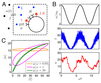
Setup

We consider a minimal sensory module (Fig. 1A): Ligand molecules $\mathrm{L}$ are inserted into a reaction volume at rate $\alpha(t)$ and removed with rate constant $\beta$. A pool of $N$ receptor molecules $\mathrm{R}$ can bind and unbind ligands, with rate constants $\gamma$ and $\mu$, respectively:

$$\varnothing\underset{\beta}{\overset{\alpha(t)}{\rightleftharpoons}}\mathrm{L}{};\quad\mathrm{L}{}+\mathrm{R}\underset{\mu}{\overset{\gamma}{\rightleftharpoons}}\mathrm{LR}.$$ (1)

The rate $\alpha(t)$ dynamically creates $\ell(t)$ free ligand molecules, which drive the formation of $n(t)$ LR complexes, leaving $r(t)\equiv N-n(t)$ receptors unbound. $\ell(t)$ acts as a noisy reporter for $\alpha(t)$, which is a proxy for the background ligand concentration to be sensed by the cell. We take $\alpha(t)$ as the input and the response $n(t)$ as the output of the module.

To study how dissipation and prediction depend on the dynamics of $\alpha(t)$, we first consider the sinusoidal signal $\alpha(t)=\alpha_{0}[1+\rho\cos(\omega t)]$, with $0\leq\rho\leq 1$. The response is shown in Fig. 1B and C: The free ligand number $\ell(t)$ oscillates around its mean $\lambda_{0}\equiv\alpha_{0}/\beta$ stochastically and, for sufficiently fast ligand exchange, in phase with $\alpha(t)$. The output $n(t)$ is damped and lags behind the signal, depending on the binding speed $\mu/\omega$, which is the primary design parameter.

The stochastic dynamics are given by the Master equation

$$\partial_{t}p(\ell,n|t)=\bigl{(}{\cal B}_{\ell}^{\alpha(t),\beta}+{\cal A}_{\ell,n}^{\gamma,\mu,N}\bigr{)}p(\ell,n|t).$$ (2)

Here ${\cal B}_{\ell}^{\alpha,\beta}=\alpha(\mathcal{E}^{-}_{\ell}-1)+\beta(\mathcal{E}^{+}_{\ell}-1)\ell$, ${\cal A}_{\ell,n}^{\gamma,\mu,N}=\gamma(\mathcal{E}^{+}_{\ell}\mathcal{E}^{-}_{n}-1)\ell r+\mu(\mathcal{E}^{-}_{\ell}\mathcal{E}^{+}_{n}-1)n$, and $\mathcal{E}^{\pm}_{x}f(x)=f(x_{\pm})$ define the birth-death ligand exchange, ligand association, and step operators, respectively, and $x_{\pm}\equiv x\pm 1$. Appropriate boundary conditions enforce $\ell\geq 0$ and $0\leq n\leq N$.

Dissipated heat

To characterize the thermodynamics Nicolis and Prigogine (1977); Schnakenberg (1976); Gaspard (2004); Hill (2004); Schmiedl and Seifert (2007) of our module, we require all reactions to be elementary, i.e. without implicit dissipative steps such as ATP turnover Seifert (2012). If $\alpha(t)=\alpha$ were a constant, the stationary solution of Eq. 2 would take the thermodynamic equilibrium form van Kampen (1992) $p_{\mathrm{eq}}(\ell,n)\propto z^{\ell}_{\mathrm{L}}{}z^{r}_{\mathrm{R}}z^{n}_{\mathrm{LR}}/(\ell!r!n!)$, where detailed balance requires $z_{\mathrm{L}}{}=\alpha/\beta$ and $z_{\mathrm{LR}}/z_{\mathrm{R}}=\alpha\gamma/(\beta\mu)$, and $z_{\mathrm{R}}$ is fixed by normalization. The Gibbs free energy $\Phi=-\log p_{\mathrm{eq}}$ would be (in $k_{\rm B}T$ units, up to a constant)

$$\Phi =\log(\ell!r!n!)-(\ell+n)\log(\alpha/\beta)-n\log(\gamma/\mu).$$ (3)

When driven out of equilibrium by a dynamic rate $\alpha(t)$, the network responds with a non-equilibrium distribution $p(\ell,n|t)$. Importantly, $\Phi(\ell,n,t)$ remains meaningful as the free energy associated with equilibrium at the current $\alpha(t)$.

After transient relaxation, the system approaches a periodic state, where

$$0 =\oint dt\,\frac{d}{dt}\langle\Phi\rangle=\oint dt\,\frac{d}{dt}\sum_{\ell n}p(\ell,n|t)\Phi(\ell,n,t)$$

$$=\oint d\alpha(t)\,\langle\partial_{\alpha}\Phi\rangle+\oint dt\,\sum_{\ell n}\left[\partial_{t}p(\ell,n|t)\right]\Phi(\ell,n,t)$$

$$\equiv W+(-Q).$$ (4)

Here $\oint\equiv\int_{t}^{t+T}$ integrates over a period, and $\langle\cdot\rangle$ averages over $p(\ell,n|t)$. We recognize $W$ as the average chemical work that the external forcing $\alpha(t)$ performs on the system over the course of a cycle, Fig. 2A. We rewrite $Q$ using Eq. 2 as

$$Q =\oint dt\,\sum_{\ell n}\bigl{[}J_{\ell n}^{\ell_{+}n}\bigl{(}-\Delta\Phi_{\ell n}^{\ell_{+}n}\bigr{)}+J_{\ell n}^{\ell_{-}n_{+}}\bigl{(}-\Delta\Phi_{\ell n}^{\ell_{-}n_{+}}\bigr{)}\bigr{]}$$

$$\equiv Q_{\mathrm{exch}}+Q_{\mathrm{bind}},$$ (5)

where $J_{\ell n}^{\ell_{+}n}=\alpha(t)p(\ell|t)-\beta\ell_{+}p(\ell_{+}|t)$ and $J_{\ell n}^{\ell_{-}n_{+}}=\gamma\ell rp(\ell,n|t)-\mu n_{+}p(\ell_{-},n_{+}|t)$ are the net probability fluxes for ligand exchange and ligand binding, respectively. Eq. 5 allocates the dissipated heat per cycle to free-energy drops $-\Delta\Phi^{n^{\prime}\ell^{\prime}}_{n\ell}=\Phi(n,\ell,t)-\Phi(n^{\prime},\ell^{\prime},t)$ occurring in the reaction events. Eq. Dissipated heat thus states the first law: The net applied work $W$ over a cycle is dissipated into the thermal bath as heat $Q$ by the reactions.

Figure 2: Dissipation and prediction in the high copy-number regime. (A) Dissipated heat is the area of the cycle defined by the thermodynamic force $-\partial_{\alpha}\langle\Phi\rangle$ and the driving function $\alpha(t)$. (B) Frequency matching $\mu=\omega$ maximizes heat. (C) Perfect tracking $\mu\to\infty$ maximizes near-future predictive information (small $\tau$), while frequency matching $\mu\simeq\omega$ maximizes far-future predictive information (large $\tau$). (D) Phase diagram of information-optimal $\mu^{*}/\omega$ vs. $\tau$ reveals transition at $\tau_{c}$, beyond which optimal prediction can be maximally dissipative. Parameters are $\rho=0.5$ and $\nu_{0}=10$.

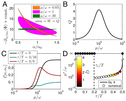
We assume throughout that ligand exchange fluxes dominate over binding fluxes, i.e. binding is effectively reaction limited. We thus require $\beta\gg\gamma\nu_{0}$ and $\alpha_{0}\gg\mu\nu_{0}$ sup , where $\nu_{0}$ is the time-average of $n(t)$. Then $\ell(t)$ is unperturbed by the receptor state: $\partial_{t}p(\ell|t)\simeq{\cal B}_{\ell}^{\alpha(t),\beta}p(\ell|t)$. We further suppose that ligand numbers respond instantaneously to the input, $\beta\gg\omega$. Under these two assumptions, $\ell$ is Poisson distributed with mean $\langle\ell(t)\rangle=\alpha(t)/\beta$, and ligand exchange is non-dissipative, $Q_{\mathrm{exch}}=0$ sup . Evaluating $W$ using Eq. 3, the energy balance Eq. Dissipated heat simplifies to

$$-\oint d\alpha(t)\,\langle n\rangle/\alpha=W=Q_{\mathrm{bind}}.$$ (6)

Predictive information

To assess the sensory performance of the module, we ask a biologically motivated question: At time $t$, how much does the output $n=n(t)$ enable the cell to prepare for the future environmental state $\alpha_{\tau}\equiv\alpha(t+\tau)$? The answer is given by the mutual information (in nats),

$$I[n,\alpha_{\tau}]=\int d\alpha_{\tau}\sum_{n}p(n,\alpha_{\tau})\log\Bigl{[}\frac{p(n,\alpha_{\tau})}{p(n)p(\alpha_{\tau})}\Bigr{]},$$ (7)

which is the reduction in uncertainty about $\alpha_{\tau}$, given $n$ . Here $p(n,\alpha_{\tau})=\oint dt\,p[n(t),\alpha(t+\tau)|t]p(t)$, and $p(t)=1/T$ corresponds to picking a sampling time at random, or equivalently to sensing a signal of unknown phase.

High copy-number limit

To gain intuition, we first consider the effect of varying response speed $\mu/\omega$ on dissipation and predictive information in a high copy-number limit sup . Specifically, we let $\{\lambda_{0},N\}\to\infty$ and $\gamma\to 0$ such that the mean number of bound receptors $\nu_{0}=\gamma\lambda_{0}N/\mu$ remains constant. The solution $p(n|t)$ is known to be a Poisson distribution Gardiner (2004); Mugler et al. (2010) with a mean $\langle n(t)\rangle=\nu_{0}\{1+\rho\delta\cos[\omega(t-\Lambda)]\}$ that lags behind the driving by $\Lambda\equiv\tan^{-1}(\omega/\mu)/\omega$ and is damped by a factor $\delta\equiv[1+(\omega/\mu)^{2}]^{-1/2}$.

In this limit, we compute the total heat dissipation by using $\langle n(t)\rangle$ with Eq. 6, as

$$Q=2\pi\bigl{[}1-\sqrt{1-\rho^{2}}\bigr{]}\nu_{0}\frac{\mu/\omega}{1+(\mu/\omega)^{2}},$$ (8)

shown in Fig. 2B. Maximum heat dissipation occurs for frequency-matched $\mu=\omega$, at lag $\Lambda=T/8$. Fast $\mu/\omega\to\infty$ allows instant tracking of the input, dissipating no heat; while slow $\mu/\omega\to 0$ produces no response, also dissipating no heat.

Dissipative optimal prediction

The predictive information, evaluated numerically using the known Poissonian $p(n|t)$ sup , is shown as a function of the receptor speed $\mu/\omega$ in Fig. 2C. Its shape depends strongly on the desired prediction interval $\tau$. As may be expected, instantaneous sensing ($\tau=0$) works best when receptor binding tracks the input at $\mu/\omega\to\infty$, without dissipation. Surprisingly, for finite $\tau=3T/8$, the prediction performance has a pronounced optimum at a frequency-matched response with $\mu\simeq\omega$. Thus, long-term prediction can be optimal at maximum dissipation. This is our principal observation.

Furthermore, the phase diagram Fig. 2D shows that the optimal prediction strategy switches from non-dissipative $\mu^{*}=\infty$ to maximally dissipative $\mu^{*}\simeq\omega$, as the forecast interval exceeds a critical value $\tau_{c}$. The discontinuity arises from a secondary local maximum in $I$ that develops for increasing $\tau$ (cf. Fig. 2C) and exceeds the plateau value at $\mu\to\infty$ when $\tau\geq\tau_{c}$. Expanding $p(n|t)$ in Fourier modes in $t$ and its natural eigenmodes in $n$ sup , we obtain

$$I[n,\alpha_{\tau}]=\frac{\rho^{2}\nu_{0}}{4}\Bigl{[}\frac{(\mu/\omega)^{2}\cos(\omega\tau)-\mu/\omega\sin(\omega\tau)}{1+(\mu/\omega)^{2}}\Bigr{]}^{2}$$ (9)

to leading order in the driving amplitude. This expression indeed has a local maximum at $\mu^{*}/\omega=\sin(\omega\tau)/[\cos(\omega\tau)+1]$ that becomes global when $\tau>\tau_{c}=T\cos^{-1}(1/3)/(2\pi)\simeq 0.2T$ (Fig. 2D).

A second surprising feature of Fig. 2C is that in the frequency-matched regime $\mu\simeq\omega$, the predictive information at $\tau=3T/8$ is higher than the instantaneous information at $\tau=0$. Counterintuitively, the system can contain more information about the future than about the present.

Figure 3: Prediction through memory. (A) For a range of prediction intervals $\tau$, frequency matching $\mu=\omega$ is more predictive than perfect tracking $\mu\to\infty$. The reason, as demonstrated by $p(n,\alpha_{\tau})$ at key points (B-E as indicated in A) and illustrated in F, is memory: receptors with $\mu=\omega$ time-integrate the signal, so that $n(t)$ lags by $\Lambda$; it is maximally correlated with $\alpha(t-\Lambda)$, which in turn mirrors $\alpha(t-\Lambda+T/2)$. Parameters are $\rho=0.75$ and $\nu_{0}=30$.

Exploiting signal correlations through memory

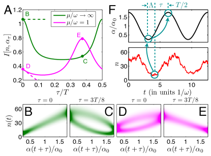
The above observations can be understood by carefully considering the connection between prediction and memory. Fig. 3A shows the predictive information $I[n,\alpha_{\tau}]$ as a function of the prediction interval, denoted $I_{\infty}(\tau)$ and $I_{\omega}(\tau)$, for fast ($\mu/\omega\to\infty$) and frequency-matched ($\mu=\omega$) response, respectively. Three features are apparent at small $\tau$. First, $I_{\infty}(0)$ is larger than $I_{\omega}(0)$, i.e. responding quickly does maximize information about the present. Second, both $I_{\infty}(\tau)$ and $I_{\omega}(\tau)$ decrease for small $\tau$, in line with a general expectation that longer-term prediction is more difficult. Third, as illustrated by the slopes in Fig. 3A (dashed lines), $\partial_{\tau}I_{\omega}\bigr{|}_{0}$ is steeper than $\partial_{\tau}I_{\infty}\bigr{|}_{0}$, which is zero. In fact, differentiating Eq. 9 with respect to $\tau$, taking $\tau\to 0$, and comparing to Eq. 8, we obtain $-\partial_{\tau}I\bigr{|}_{0}\leq Q/T$ sup , which is precisely the bound of Ref. Still et al. (2012) applied to our system.

The key point is that a surprise occurs beyond the limit $\tau\to 0$. Both curves increase again, which is a direct consequence of the sinusoidal input: When $\tau$ is a half-integer or integer multiple of $T$, $I(\tau)$ must equal $I(0)$, since then $\alpha(t+\tau)$ perfectly mirrors or tracks $\alpha(t)$, respectively. Indeed, $I(\tau)$ is $T/2$-periodic. Interestingly, the frequency-matched $I_{\omega}(\tau)$ increases sufficiently to overtake both its own initial value, and the fast-responding $I_{\infty}(\tau)$.

The takeover occurs because the lag introduced by a slower response removes an ambiguity inherent in prediction, Fig. 3B-E. While the fast response tracks the present input well (B), its predictions suffer from a two-fold ambiguity about $\alpha(t+\tau)$, since a given value of $n(t)$ maps with high probability to two distinct values of $\alpha(t+\tau)$ (C), corresponding to the rising and falling half-period. In contrast, the frequency-matched response tracks the delayed signal $\alpha(t-\Lambda)$. This introduces a two-fold ambiguity about the present signal for the same reason (D) but strikingly, helps prediction: The future signal $\alpha(t-\Lambda+T/2)$ is tracked without two-fold ambiguity (E). Indeed Fig. 3A shows that $I_{\omega}(\tau)$ is maximal when the lag, advanced by half a period, equals the prediction interval: $-\Lambda+T/2=\tau$, or, for $\Lambda=T/8$ in the maximally dissipative case, when $\tau=3T/8$. This advantage of removing ambiguity outweighs the disadvantage of a reduced response range due to damping; the net effect is an increase in predictive power over the fast response.

In essence, a dissipative system can exploit memory to achieve superior predictive power, by maximizing information of the past and therefore, due to strong signal autocorrelations, about the future (Fig. 3F).

Figure 4: Dissipative optimal prediction is generic. (A) For stochastic two-state driving with Gamma-distributed waiting times, dissipative prediction is optimal for shape parameters $k\geq 3$. (B) For driving by a non-Markovian damped harmonic oscillator, dissipative prediction is optimal in the underdamped regime $\eta=0.5$ but not at critical damping $\eta=2$ or in the overdamped regime $\eta=4$. Parameters are $\tau=3T/8$, $\rho=0.5$, $\lambda_{0}=25$, $N=25$, $\beta/\omega=100$, and $\gamma=\mu/\lambda_{0}$. Simulation details are in sup .

Dissipative optimal prediction is generic

While tractable, a sinusoidal signal is arguably too predictable. In fact, since $I(\tau)$ is periodic, the optimal prediction strategy alternates indefinitely between dissipative and non-dissipative as $\tau\to\infty$. However, dissipative optimal prediction occurs in more general contexts; we now explore what features of signal and response are necessary to observe it.

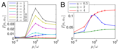
The input distribution $p(\alpha)$ for a sinusoid is peaked at the extrema, but this is not necessary: A triangle wave with uniform $p(\alpha)$ also produces the effect (not shown). High copy number is not necessary: Relaxing the high copy-number limit, we observe dissipative optimal prediction even down to $\lambda_{0}=1$ and $N=1$ sup .

Periodic and deterministic signals are not necessary. This is seen by considering two-state driving processes that switch between $\alpha_{0}(1\pm\rho)$ with waiting times that are Gamma-distributed with varying shape parameter but constant mean $T/2=\pi\omega$. Fig. 4A shows that dissipative prediction is optimal for strongly correlated two-state signals, and even for very stochastic signals down to shape parameter $k\geq 3$, but not for the Markovian random telegraph signal at $k=1$. Indeed, we find that prediction of Markovian driving signals is governed purely by the instantaneous response $p[n(t)|\alpha(t)]$, as no additional predictive information is encoded in past signal values sup .

While a non-Markovian signal appears necessary, it may be insufficient. This is seen by considering a continuous, non-Markovian driving process $\alpha(t)=\alpha_{0}[1+\rho x(t)]$ defined by the two-dimensional Langevin equation for a thermal harmonic oscillator, $\partial_{\omega t}x=p,\;\partial_{\omega t}p=-x-\eta p+\sqrt{2\eta}\xi,$ where $\xi$ is unit Gaussian white noise. This signal does not admit dissipative optimal prediction in the overdamped regime $\eta\geq\eta_{c}=2$ (Fig. 4B). Only when the driving becomes oscillatory with resonant frequency $\omega_{1}=\omega\sqrt{1-\eta^{2}/4}>0$ for $\eta<\eta_{c}$, is dissipative optimal prediction recovered.

Discussion

Our model system Eq. 1 shows that dissipation is not fundamentally required for measuring the current state of a signal. In fact, dissipation degrades instantaneous sensing by introducing ambiguity and damping the response. However, a lagging, dissipative response improves finite-time prediction by resolving ambiguities in non-Markovian signals, over a range of prediction intervals on the order of the signal period.

This may be a general mechanism for biological systems to anticipate oscillations. In cyanobacteria, the KaiABC circadian clock Johnson et al. (2011) is read out by binding of the effector kinase SasA to the oscillating phosphorylated form of KaiC. The low dissociation rate $\mu\simeq 4\times 10^{-4}/$s Valencia et al. (2012) of this complex implies a lagging response with $\mu/\omega\simeq 5$, enabling dissipative prediction. In sea urchin sperm cells, chemotaxis is performed by helical swimming up a ligand gradient, giving rise to an oscillatory ligand signal with period $T\simeq 1$ s Kaupp et al. (2008); as in Eq. 1, ligands bind and activate transmembrane receptors whose deactivation rate $\mu/\omega\simeq 0.5$ also enables dissipative prediction. Intriguingly, each ligand peak is eventually followed by a motor response after $\tau=0.4T$ Kaupp et al. (2008), such that the lagging receptor state would optimally predict the signal at the future time $t+\tau$ of the motor response (cf. Fig. 3).

In this study, energy is supplied by a dynamic input and dissipated by a passive sensory module. Many signal transduction modules dissipate energy that is supplied internally by ATP turnover. It will be interesting to explore the interplay between input-supplied and internally supplied energy and its implications for sensing and prediction.

This work is part of the research program of the “Stichting FOM”, which is financially supported by the “Nederlandse organisatie voor Wetenschappelijk Onderzoek” (NWO). NB was supported in part by a fellowship of the Heidelberg Center for Modelling and Simulation in the Biosciences (BIOMS).

Appendix A Appendix

A.1 Dominant ligand fluxes

To identify the conditions for which ligand fluxes dominate over binding fluxes, we sum Eq. 2 over $n$, obtaining (here suppressing $t$ arguments)

$$\dot{p}(\ell)={\cal B}_{\ell}^{\alpha,\beta}p(\ell)+\gamma[\langle r|\ell_{+}\rangle\ell_{+}p(\ell_{+})-\langle r|\ell\rangle\ell p(\ell)]\\ +\mu[\langle n|\ell_{-}\rangle p(\ell_{-})-\langle n|\ell\rangle p(\ell)].$$ (A1)

For moderate driving amplitude around half-filling of the receptors, the conditional averages $\langle n|\ell\rangle,\langle r|\ell\rangle$ remain close to their mean $\nu_{0}$. Therefore, taking $\beta\gg\gamma\nu_{0}$ and $\alpha_{0}\gg\mu\nu_{0}$ ensures that $\dot{p}(\ell)\simeq{\cal B}_{\ell}p(\ell)$, ie. the ligand in- and outflux terms dominate.

To see explicitly that the ligand exchange heat vanishes for fast ligand exchange, we rewrite

$$Q_{\mathrm{exch}} =\oint\sum_{\ell}[\alpha(t)p(\ell|t)-\beta\ell_{+}p(\ell_{+}|t)]\log\Bigl{[}\frac{\alpha(t)}{\beta\ell_{+}}\Bigr{]}\,dt$$

$$=\oint\bigl{(}\alpha-\beta\langle\ell\rangle\bigr{)}\log(\alpha/\beta)\,dt$$

$$\quad-\oint\sum_{\ell}\bigl{[}\alpha p(\ell|t)-\beta\ell_{+}p(\ell_{+}|t)\bigr{]}\log\ell_{+}\,dt.$$ (A2)

For fast ligand exchange, $p(\ell|t)$ is a Poisson distribution with mean $\langle\ell(t)\rangle=\alpha(t)/\beta$, so that the first integral on the right hand side of the last equality vanishes. To see that the second integral vanishes, note that the Poisson distribution satisfies $p(\ell_{+})/p(\ell)=\langle\ell\rangle/\ell_{+}$.

A.2 High copy-number limit

We let $\{\lambda_{0},N\}\to\infty$ and $\gamma\to 0$ such that the mean number of bound receptors $\nu_{0}=\gamma\lambda_{0}N/\mu$ remains constant. This ensures that $n(t)$ remains in the linear, non-saturated range of the response curve: $N\gg\nu_{0}$ implies that $r(t)=O(N-\nu_{0})=O(N)$. It also ensures that the receptors are effectively driven by a deterministic signal: The relative width of the ligand distribution decreases as $\sigma_{\ell}/\lambda_{0}=O(\lambda_{0})^{-1/2}$. The receptor dynamics thus reduce to a birth-death process, $\partial_{t}p(n|t)={\cal B}_{n}^{\tilde{\gamma}(t),\mu}p(n|t)$, with effective birth rate $\gamma\ell(t)r(t)=\gamma[\alpha(t)/\beta]N+O(\nu_{0}/N)+O(\lambda_{0}^{-1/2})$, which we denote as $\tilde{\gamma}(t)\equiv\gamma[\alpha(t)/\beta]N=\nu_{0}\mu[1+\rho\cos(\omega t)]$. The solution to a birth-death process with time-dependent birth rate $\tilde{\gamma}(t)$ is $p(n|t)=\int_{-\infty}^{0}\,dt^{\prime}e^{-\mu(t-t^{\prime})}\tilde{\gamma}(t^{\prime})=\nu_{0}\{1+\rho\delta\cos[\omega(t-\Lambda)]\}$, with lag $\Lambda\equiv\tan^{-1}(\omega/\mu)/\omega$ and damping $\delta\equiv[1+(\omega/\mu)^{2}]^{-1/2}$, as in the main text.

A.3 Analytic results for predictive information

For a deterministic signal $\alpha(t)$, we have $p(\alpha_{\tau}|n,t)=p(\alpha_{\tau}|t)=\delta[\alpha_{\tau}-\alpha(t+\tau)]$, and the predictive information (Eq. 7) becomes

$$I[n,\alpha_{\tau}]= \sum_{n}\int d\alpha_{\tau}\ p(n,\alpha_{\tau})$$

$$= \sum_{n}\int d\alpha_{\tau}\oint dt\ p(\alpha_{\tau}|n,t)p(n|t)p(t)\log\Bigl{[}\frac{p(n|\alpha_{\tau})}{p(n)}\Bigr{]}$$

$$= \sum_{n}\frac{1}{T}\oint dt\ p(n|t)\log\Bigl{[}\frac{p(n|\alpha(t+\tau))}{p(n)}\Bigr{]}.$$ (A3)

For cosine driving $\alpha(t)=\alpha(T-t)$, there is a two-to-one relationship between $t$ and $\alpha$. This yields $p(n|\alpha(t+\tau))=[p(n|t_{1})+p(n|t_{2})]/2$, where $t_{1}=t$ and $t_{2}=T-t-2\tau$ are the two time points for which $\alpha_{\tau}$ takes on the value $\alpha(t+\tau)$. The predictive information becomes

$$I[n,\alpha_{\tau}]=\sum_{n}\frac{1}{T}\oint dt\ p(n|t)\log\Bigl{[}\frac{p(n|t_{1})+p(n|t_{2})}{2p(n)}\Bigr{]}.$$ (A4)

In the high copy-number limit (Figs. 2 and 3), Eq. A4 is evaluated numerically using the Poissonian $p(n|t)$ with mean $\langle n(t)\rangle=\nu_{0}\{1+\rho\delta\cos[\omega(t-\Lambda)]\}$, time lag $\Lambda\equiv\tan^{-1}(\omega/\mu)/\omega$, and damping factor $\delta\equiv[1+(\omega/\mu)^{2}]^{-1/2}$.

To get analytical insight, we can expand Eq. A4 in the limit of small driving amplitude $\rho$. To facilitate the expansion, we exploit the fact that $p(n|t)$ can be expressed Mugler et al. (2010) in terms of its Fourier modes in $t$,

$$p(n|t)=\sum_{z=-\infty}^{\infty}p_{n}^{z}e^{-iz\omega t},$$ (A5)

and its natural eigenmodes in $n$,

$$p_{n}^{z}=e^{iz\omega\Lambda}\sum_{j=0}^{\infty}\frac{(\nu_{0}\rho\delta/2)^{2j+|z|}}{j!(j+|z|)!}\phi_{n}^{2j+|z|}.$$ (A6)

Here $p_{n}^{z}=(1/T)\int_{0}^{T}dt\ e^{iz\omega t}p(n|t)$ are the components of the Fourier transform, which have support only at integer multiples $z$ of the driving frequency, and $\phi_{n}^{j}$ are the eigenmodes of the static birth-death process with mean bound receptor number $\nu_{0}$, i.e. $-{\cal B}_{n}^{\nu_{0},1}\phi_{n}^{j}=j\phi_{n}^{j}$ for eigenvalues $j\in\{0,1,\dots,\infty\}$ Walczak et al. (2009). Eq. A6 shows directly that the distribution is expressible as an expansion in the small parameter $\rho$. The remaining task is then to identify the leading term in $\rho$.

To identify the leading term in $\rho$, we insert Eq. A5 into Eq. A4, which yields

$$I = \frac{1}{T}\sum_{n}\int_{0}^{T}dt\ \sum_{z}p_{n}^{z}e^{-iz\omega t}$$ (A7)

$$\times\log\left\{\frac{1}{2p_{n}^{0}}\sum_{z^{\prime}}p_{n}^{z^{\prime}}\left[e^{-iz^{\prime}\omega t}+e^{-iz^{\prime}\omega(T-2\tau-t)}\right]\right\}.\qquad$$

Here we have recognized that $p(n)$, which is the time average of $p(n|t)$, is also the zeroth Fourier mode: $p(n)=\int_{0}^{T}dt\ p(n|t)p(t)=(1/T)\int_{0}^{T}dt\ p(n|t)=p_{n}^{0}$. Isolating the $z^{\prime}=0$ term and defining $q_{n}^{z}\equiv p_{n}^{z}e^{iz\omega\tau}$ to make the expression more symmetric yields

$$I = \frac{1}{T}\sum_{n}\int_{0}^{T}dt\ \sum_{z}p_{n}^{z}e^{-iz\omega t}$$ (A8)

$$\times\log\left\{1+\frac{1}{2p_{n}^{0}}\sum_{z^{\prime}\neq 0}q_{n}^{z^{\prime}}\left[e^{-iz^{\prime}\omega(t+\tau)}+e^{iz^{\prime}\omega(t+\tau)}\right]\right\},\qquad$$

where we have recognized that $e^{-iz^{\prime}\omega T}=1$. Then, recognizing that the term in brackets is symmetric upon $z^{\prime}\to-z^{\prime}$, we write the $z^{\prime}$ sum in terms of only positive integers,

$$I = \frac{1}{T}\sum_{n}\int_{0}^{T}dt\ \sum_{z}p_{n}^{z}e^{-iz\omega t}$$ (A9)

$$\times\log\left\{1+\frac{1}{2p_{n}^{0}}\sum_{z^{\prime}>0}r_{n}^{z^{\prime}}\left[e^{-iz^{\prime}\omega(t+\tau)}+e^{iz^{\prime}\omega(t+\tau)}\right]\right\},\qquad$$

where

$$r_{n}^{z} \equiv q_{n}^{z}+q_{n}^{-z}$$ (A10)

$$= e^{iz\omega\tau}p_{n}^{z}+e^{-iz\omega\tau}p_{n}^{-z}$$

$$= \left[e^{iz\omega(\Lambda+\tau)}+e^{-iz\omega(\Lambda+\tau)}\right]\sum_{j}\frac{(\nu_{0}\rho\delta/2)^{2j+|z|}}{j!(j+|z|)!}\phi_{n}^{2j+|z|}$$

$$= 2\cos[z\omega(\Lambda+\tau)]\sum_{j}\frac{(\nu_{0}\rho\delta/2)^{2j+|z|}}{j!(j+|z|)!}\phi_{n}^{2j+|z|}$$

is a real quantity.

Now, since $r_{n}^{z}$ is expressed in terms of our small parameter $\rho$, we Taylor expand the log in Eq. A9:

$$I = \frac{1}{T}\sum_{n}\int_{0}^{T}dt\ \sum_{z}p_{n}^{z}e^{-iz\omega t}\sum_{k=1}^{\infty}\frac{(-1)^{k+1}}{k}$$ (A11)

$$\times\left\{\frac{1}{2p_{n}^{0}}\sum_{z^{\prime}>0}r_{n}^{z^{\prime}}\left[e^{-iz^{\prime}\omega(t+\tau)}+e^{iz^{\prime}\omega(t+\tau)}\right]\right\}^{k}.\quad$$

It will turn out that the first two terms in the Taylor expansion will contribute to the leading order in $\rho$. The first term ($k=1$) is

$$I^{(1)} = \sum_{n}\frac{1}{2p_{n}^{0}}\sum_{z^{\prime}>0}r_{n}^{z^{\prime}}\sum_{z}p_{n}^{z}$$ (A12)

$$\times\frac{1}{T}\int_{0}^{T}dt\ e^{-iz\omega t}\left[e^{-iz^{\prime}\omega(t+\tau)}+e^{iz^{\prime}\omega(t+\tau)}\right],\qquad$$

where we have reordered terms in preparation for exploiting the relation $(1/T)\int_{0}^{T}dt\ e^{-i(z-z^{\prime})\omega t}=\delta_{zz^{\prime}}$. This relation turns the two terms in brackets into Kronecker deltas, which each collapse the sum over $z$, leaving

$$I^{(1)} = \sum_{n}\frac{1}{2p_{n}^{0}}\sum_{z^{\prime}>0}r_{n}^{z^{\prime}}\left(e^{-iz^{\prime}\omega\tau}p_{n}^{-z^{\prime}}+e^{iz^{\prime}\omega\tau}p_{n}^{z^{\prime}}\right)$$ (A13)

$$= \frac{1}{2}\sum_{n}\frac{1}{p_{n}^{0}}\sum_{z^{\prime}>0}(r_{n}^{z^{\prime}})^{2}.$$

In a completely analogous way, the second term in the Taylor expansion ($k=2$) reduces to

$$I^{(2)}=-\frac{1}{8}\sum_{n}\frac{1}{\left(p_{n}^{0}\right)^{2}}\sum_{x>0}\sum_{y>0}r_{n}^{x}r_{n}^{y}\left(r_{n}^{x+y}+r_{n}^{x-y}\right).$$ (A14)

Considering the $j=0$ term in $r_{n}^{z}$ (Eq. A10), it is clear that the leading order behavior in $\rho$, proportional to $\rho^{2}$, comes from the $z^{\prime}=1$ term in Eq. A13 and the $x=y=1$ term in Eq. A14:

$$I \approx \frac{1}{2}\sum_{n}\frac{1}{p_{n}^{0}}(r_{n}^{1})^{2}-\frac{1}{8}\sum_{n}\frac{1}{\left(p_{n}^{0}\right)^{2}}r_{n}^{1}r_{n}^{1}\left(r_{n}^{0}\right)$$ (A15)

$$= \frac{1}{2}\sum_{n}\frac{(r_{n}^{1})^{2}}{r_{n}^{0}}$$ (A16)

$$\approx \cos^{2}[\omega(\Lambda+\tau)]\left(\frac{\nu_{0}\rho\delta}{2}\right)^{2}\sum_{n}\frac{(\phi_{n}^{1})^{2}}{\phi_{n}^{0}}$$ (A17)

$$= \frac{\nu_{0}^{2}\rho^{2}}{4}\left[\frac{\cos(\omega\tau)-(\omega/\mu)\sin(\omega\tau)}{1+(\omega/\mu)^{2}}\right]^{2}\sum_{n}\frac{(\phi_{n}^{1})^{2}}{\phi_{n}^{0}}.\qquad$$ (A18)

Here, Eq. A16 uses the fact that $r_{n}^{0}=2p_{n}^{0}$ (Eq. A10), Eq. A17 takes only the $j=0$ term in Eq. A10, and Eq. A18 recalls that $\delta=[1+(\omega/\mu)^{2}]^{-1/2}$ and uses

$$\cos[\omega(\Lambda+\tau)] = \cos(\omega\Lambda)\cos(\omega\tau)-\sin(\omega\Lambda)\sin(\omega\tau)$$ (A19)

$$= \cos\left[\tan^{-1}(\omega/\mu)\right]\cos(\omega\tau)$$

$$-\sin\left[\tan^{-1}(\omega/\mu)\right]\sin(\omega\tau)$$

$$= \frac{1}{\sqrt{1+(\omega/\mu)^{2}}}\cos(\omega\tau)$$

$$-\frac{\omega/\mu}{\sqrt{1+(\omega/\mu)^{2}}}\sin(\omega\tau).$$

The sum in Eq. A18 is evaluated by noting that the zeroth eigenmode is a Poisson distribution with mean $\nu_{0}$ and that the first eigenmode is related to the zeroth eigenmode via $\phi_{n}^{1}=\phi_{n-1}^{0}-\phi_{n}^{0}=\phi_{n}^{0}(n-\nu_{0})/\nu_{0}$ Mugler et al. (2009). The sum therefore becomes $(1/\nu_{0}^{2})\sum_{n}\phi_{n}^{0}(n-\nu_{0})^{2}$, which is the variance of the Poisson distribution (equal to $\nu_{0}$) divided by $\nu_{0}^{2}$, or $1/\nu_{0}$. Altogether, then, Eq. A18 becomes

$$I=\frac{\nu_{0}\rho^{2}}{4}\left[\frac{\cos(\omega\tau)-(\omega/\mu)\sin(\omega\tau)}{1+(\omega/\mu)^{2}}\right]^{2},$$ (A20)

as in Eq. 9.

A.4 Dissipation bounds instantaneous prediction

In the high copy-number and small-amplitude driving limits, $I$ is given by Eq. A20. Differentiating Eq. A20 with respect to $\tau$ and evaluating at $\tau=0$ obtains

$$\partial_{\tau}I\big{|}_{0}=\frac{\nu_{0}\rho^{2}\omega}{2}\frac{\omega/\mu}{[1+(\omega/\mu)^{2}]^{2}}.$$ (A21)

Dissipated heat in the high copy-number limit is given by Eq. 8. In the small-amplitude limit, we take Eq. 8 to leading order in $\rho$:

$$Q=\pi\rho^{2}\nu_{0}\frac{\mu\omega}{\mu^{2}+\omega^{2}}.$$ (A22)

Using $T=2\pi/\omega$, Eqs. A21 and A22 satisfy

$$-\partial_{\tau}I\big{|}_{0}=\frac{Q/T}{1+(\omega/\mu)^{2}}.$$ (A23)

Since $[1+(\omega/\mu)^{2}]^{-1}\leq 1$ always, we obtain $-\partial_{\tau}I|_{0}\leq Q/T$, i.e. the dissipation bounds the instantaneous rate of change of the predictive information, as in Still et al. (2012).

A.5 Robustness to low copy-number effects

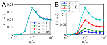
We here relax the assumption of high copy number and solve numerically the full description of the system given by Eq. 2. We find that dissipative prediction remains optimal as the mean ligand number $\lambda_{0}$ and the total receptor number $N$ are reduced, even down to $\lambda_{0}=1$ (Fig. A1A) and $N=1$ (Fig. A1B). As $N$ is reduced, the information is reduced for all values of the response rate $\mu$ (B), since reducing $N$ compresses the response range. As $\lambda_{0}$ is reduced, the information is largely unchanged (A); this is because ligand exchange remains faster than the driving dynamics ($\beta/\omega\gg 1$), meaning that even a small number of ligand molecules can cycle in and out of the system many times over a period. In both cases, there remains an optimum in the predictive information as a function of $\mu$ located in the dissipative regime $\mu\simeq\omega$, illustrating that dissipative optimal prediction persists even at low copy numbers.

Figure A1: Dissipative optimal prediction persists (A) for low mean ligand number $\lambda_{0}$ and (B) for low total receptor number $N$. Parameters are $\tau=3T/8$, $\rho=0.5$, $\beta/\omega=100$, $\gamma=\mu/\lambda_{0}$, and, in A, $N=5$ and, in B, $\lambda_{0}=5$. In A, all curves closely overlap.

A.6 Dissipative prediction and Markovian driving

We investigate whether dissipative sensing can in principle improve the prediction of Markovian inputs. In this section, we will denote the full signal history up to but excluding $t$ by $[\alpha]$, the present signal by $\alpha=\alpha(t)$, the present output by $n=n(t)$, and a future signal by $\alpha_{\tau}=\alpha(t+\tau)$, respectively.

For the sensing module studied here, the output depends only on past signal values and does not feed back onto the signal. This implies that the future trajectory of the signal does not depend on the particular response of the output: $p(\alpha_{\tau}|n,[\alpha],\alpha,t)=p(\alpha_{\tau}|[\alpha],\alpha,t)$. In other words, the output cannot give any information about the future signal in excess of what’s contained in the signal history. This relation is valid irrespective of the type of input signal.

We can then rewrite the predictive two-point distribution $p(\alpha_{\tau},n|\alpha,t)$ as an integral over the driving history:

$$p(\alpha_{\tau},n|\alpha,t) =\int\mathcal{D}[\alpha]p(\alpha_{\tau},n,[\alpha]|\alpha,t)$$

$$=\int\mathcal{D}[\alpha]p(\alpha_{\tau}|n,[\alpha],\alpha,t)$$

$$\hphantom{\sum\sum}\times p(n|[\alpha],\alpha,t)p([\alpha]|\alpha,t)$$

$$=\int\mathcal{D}[\alpha]p(\alpha_{\tau}|[\alpha],\alpha,t)$$

$$\hphantom{\sum\sum}\times p(n|[\alpha],\alpha,t)p([\alpha]|\alpha,t),$$ (A24)

where the second equality factorizes the integrand using the rule $p(x,y|z)=p(x|y,z)p(y|z)$, and the last equality uses the no-feedback relation given above.

If the response is instantaneous (adiabatic), we have the relation $p(n|[\alpha],\alpha,t)=p(n|\alpha,t)$; if the input is Markovian, $p(\alpha_{\tau}|[\alpha],\alpha,t)=p(\alpha_{\tau}|\alpha,t)$. In both cases we can integrate Eq. A.6 over $[\alpha]$ trivially and obtain the result:

$$p(\alpha_{\tau},n|\alpha,t)=p(n|\alpha,t)p(\alpha_{\tau}|\alpha,t).$$ (A25)

When the driving process is stationary, the time dependence in Eq. A25 disappears, and we can write

$$p(\alpha_{\tau},n|\alpha)=p(n|\alpha)p(\alpha_{\tau}|\alpha).$$ (A26)

Thus the basic observation is that for instantaneous response or Markovian input, $\alpha_{\tau}$ and $n$ are independent when conditioned on $\alpha$; or equivalently, the variables $n\leftrightarrow\alpha\leftrightarrow\alpha_{\tau}$ form a Markov chain Cover and Thomas (2012). In the following we consider only Markovian input. We may then insert a further input variable at an intermediate future time to extend the Markov chain as $n\leftrightarrow\alpha\leftrightarrow\hat{\alpha}\leftrightarrow\alpha_{\tau}$.

The information processing inequality states that mutual information across a Markov chain is bounded from above by the mutual information across any subchain. In particular, $I[n,\alpha_{\tau}]\leq I[n,\hat{\alpha}]$. By inserting $\hat{\alpha}$ at arbitrary intermediate times, this implies that $I(\tau)=I[n,\alpha_{\tau}]$ decreases monotonically as a function of the prediction interval. Thus, for Markovian driving, the output can never contain more information about the future than about the present signal. This is in contrast to the non-monotonic behavior shown in Fig. 3A for a deterministic signal, and also observed for the noisy non-Markovian signals we studied (not shown).

The information processing inequality further yields $I[n,\alpha_{\tau}]\leq I[\alpha,\alpha_{\tau}]$: Predictions based on measuring $n$ cannot surpass those based on the current input $\alpha$. This means that encoding the history of a Markovian signal by means of a dissipative response has no intrinsic value. Alternatively, rewriting $p(n,\alpha,\alpha_{\tau})=p(\alpha,\alpha_{\tau})p(n|\alpha)$, shows that the properties of the response enter only via the instantaneous distribution $p(n|\alpha)$, so that any memory is irrelevant for the prediction performance.

The preceding argument does not prove that a lagging response is always disadvantageous for Markovian input, but only that it is possible in principle to construct an instantaneous, non-dissipative system which is as good a predictor as any given lagging system. Nonetheless, in the cases we studied, a fast response always produced better predictors of Markovian input signals than a lagging response.

A.7 Parameters and details of the simulations

The data for Figs. 4A and B were generated by a Gillespie-type kinetic Monte Carlo simulation. Dynamic ligand birth rates $\alpha(t)$ were approximated as constant during short discretization intervals of length $\tau_{\alpha}=T/50$; after each such interval, queued next reaction times were erased and re-generated according to the new value of the rate. This is an exact simulation procedure for the approximated system with stepwise-constant rate. We found that the dissipated heat due to ligand exchange $Q_{\mathrm{exch}}$ does depend on $\tau_{\alpha}$ and requires much finer rate discretization to vanish (as required by Eq. A.1). Here, we were interested mainly in $Q_{\mathrm{bind}}$ which was found to be independent of $\tau_{\alpha}$ even down to $\tau_{\alpha}\simeq T/10$. Therefore a finer discretization was not deemed necessary.

For the two-state driving protocol (Fig. 4A), the mean ligand number and total receptor number were set to $\lambda_{0}=N=25$. The ligand death rate was set to $\beta=100$, and the mean driving period was set to $T=2\pi$ in simulation time units. Switching times were generated independently, following a Gamma- (or Erlang-) distribution with shape parameter $k\in\{1,2,3,5,10,20,50\}$ and mean $T/2$. The input rate was set to a random initial value $\alpha_{0}[1\pm\rho]$ and then toggled after each random switching time between $\alpha_{0}[1\pm\rho]$, where $\alpha_{0}=\lambda_{0}\beta$ and $\rho=0.5$. For a given ligand dissociation rate constant $\mu$, the association constant was set to $\gamma=\mu/\lambda_{0}$ to ensure half-filling at the average driving rate.

For the harmonic-oscillator protocol (Fig. 4B) the same parameters were used, except that the driving signal was now generated by a forward-Euler integration of the Langevin equation given in the main text. The damping parameter $\eta$ was varied in $\{1/2,1,2,4\}$.

For each value of $\mu$, the system state was initialized to the equilibrium molecule numbers at $\alpha=\alpha_{0}$, and $N_{\mathrm{tr}}=2000$ trajectories of length $10T$ were generated. The dissipated heat contributions $-\Delta\Phi$ (Eq. 5) were accumulated on every reaction and averaged to yield $Q_{\mathrm{bind}}$.

Trajectories were sampled at discrete time intervals $T/100$, and the corresponding samples of the input rate were binned. The input-output mutual information was estimated by applying the definition Eq. 7 to the binned simulation data. In doing so, the choice of bin size for the continuous variable $\alpha$ (in the harmonic-oscillator case) can lead to systematic errors; we found the results for $I$ to be independent of the bin size in a plateau region around $N_{\mathrm{bin}}=100$ equally filled bins, and therefore used this binning for Fig. 4B.

The data were split into 10 blocks of 200 trajectories each and the mutual information $I[n,\alpha_{\tau}]$ for various prediction intervals $\tau\in[0,T/2]$ were calculated based on histograms of the discrete-valued samples, for each block. Plots show the averages over blocks together with standard errors of the mean estimated from block-wise variation.

References

- Mitchell et al. (2009) A. Mitchell, G. H. Romano, B. Groisman, A. Yona, E. Dekel, M. Kupiec, O. Dahan, and Y. Pilpel, Nature 460, 220 (2009).
- Scialdone et al. (2013) A. Scialdone, S. T. Mugford, D. Feike, A. Skeffington, P. Borrill, A. Graf, A. M. Smith, and M. Howard, Elife 2, e00669 (2013).
- Bialek (2012) W. Bialek, Biophysics: Searching for Principles (Princeton Univ Pr, 2012).
- Still et al. (2012) S. Still, D. A. Sivak, A. J. Bell, and G. E. Crooks, Physical Review Letters 109, 120604 (2012).
- Kaupp et al. (2008) U. B. Kaupp, N. D. Kashikar, and I. Weyand, Annual Review of Physiology 70, 93 (2008).
- Valencia et al. (2012) J. Valencia, S., K. Bitou, K. Ishii, R. Murakami, M. Morishita, K. Onai, Y. Furukawa, K. Imada, K. Namba, and M. Ishiura, Genes to Cells 17, 398 (2012).
- Skoge et al. (2013) M. Skoge, S. Naqvi, Y. Meir, and N. S. Wingreen, Physical Review Letters 110, 248102 (2013).
- Detwiler et al. (2000) P. B. Detwiler, S. Ramanathan, A. Sengupta, and B. I. Shraiman, Biophysical Journal 79, 2801 (2000).
- Qian and Reluga (2005) H. Qian and T. C. Reluga, Physical Review Letters 94, 028101 (2005).
- Mehta and Schwab (2012) P. Mehta and D. J. Schwab, Proceedings of the National Academy of Sciences (2012), 10.1073/pnas.1207814109.
- Lan et al. (2012) G. Lan, P. Sartori, S. Neumann, V. Sourjik, and Y. Tu, Nature Physics 8, 422 (2012).
- Barato et al. (2013) A. Barato, D. Hartich, and U. Seifert, Physical Review E 87, 042104 (2013).
- Govern and ten Wolde (2013) C. C. Govern and P. R. ten Wolde, “How biochemical resources determine fundamental limits in cellular sensing,” (2013), arXiv:1308.1449 .
- Nicolis and Prigogine (1977) G. Nicolis and I. Prigogine, Self-organization in nonequilibrium systems (Wiley, 1977).
- Schnakenberg (1976) J. Schnakenberg, Reviews of Modern Physics 48, 571 (1976).
- Gaspard (2004) P. Gaspard, J Chem Phys 120, 8898 (2004).
- Hill (2004) T. L. Hill, Free Energy Transduction and Biochemical Cycle Kinetics (Dover Publications, 2004).
- Schmiedl and Seifert (2007) T. Schmiedl and U. Seifert, J Chem Phys 126, 044101 (2007).
- Seifert (2012) U. Seifert, Reports on Progress in Physics 75, 126001 (2012).
- van Kampen (1992) N. G. van Kampen, Stochastic Processes in Physics and Chemistry, 2nd ed. (North-Holland, 1992).
- (21) See supplementary information.
- Note (1) We note that Eq. 7 is distinct from both the predictive information between entire past and future trajectories Bialek et al. (2001) and the information rate between input and output trajectories Tostevin and ten Wolde (2009); instead, Eq. 7 focuses on a particular time point shifted by into the future.
- Gardiner (2004) C. Gardiner, Handbook of Stochastic Methods: for Physics, Chemistry and the Natural Sciences, 3rd ed. (Springer, 2004).
- Mugler et al. (2010) A. Mugler, A. M. Walczak, and C. H. Wiggins, Phys. Rev. Lett. 105, 058101 (2010).
- Johnson et al. (2011) C. H. Johnson, P. L. Stewart, and M. Egli, Annual review of biophysics 40, 143 (2011).
- Bialek et al. (2001) W. Bialek, I. Nemenman, and N. Tishby, Neural Comput 13, 2409 (2001).
- Tostevin and ten Wolde (2009) F. Tostevin and P. R. ten Wolde, Phys Rev Lett 102, 218101 (2009).
- Walczak et al. (2009) A. M. Walczak, A. Mugler, and C. H. Wiggins, Proceedings of the National Academy of Sciences 106, 6529 (2009).
- Mugler et al. (2009) A. Mugler, A. M. Walczak, and C. H. Wiggins, Phys. Rev. E 80, 41921 (2009).
- Cover and Thomas (2012) T. M. Cover and J. A. Thomas, Elements of information theory (John Wiley & Sons, 2012).