Some remarks on non-planar Feynman diagrams

Abstract

Two criteria for planarity of a Feynman diagram upon its propagators (momentum flows) are presented. Instructive Mathematica programs that solve the problem and examples are provided. A simple geometric argument is used to show that while one can planarize non-planar graphs by embedding them on higher-genus surfaces (in the example it is a torus), there is still a problem with defining appropriate dual variables since the corresponding faces of the graph are absorbed by torus generators.

02.70.Wz, 12.38.Bx, 02.10.Ox

1 Introduction

Non-planar Feynman diagrams arise naturally from perturbative quantum field theory. They are interesting for many reasons. First of all, from the graph-theoretical point of view many constructions and theorems are formulated only for planar graphs. Formally, any Feynman diagram $G$ can be considered as a graph and thus subjected to graph-theoretical methods. Moreover, labelling all edges of $G$ by momenta makes $G$ a network flow, and which is not necessarily unique. Consequently, it can make some redundant problems on the way to find effective analytical or numerical solutions to a given Feynman diagram. This is especially true if we want to make general programs which use some methods to solve Feynman integrals. We focus here on one technical aspect. Given a Feynman diagram $G$, is it possible to decide the planarity of $G$ only upon its propagators? The question could be rewritten in a more general way: is it possible to decide the planarity of a network flow only upon its flows? The answer is important considering e.g. computer algebra methods in particle physics. We faced the problem when working on the upgrade of AMBRE package [1], where different methods are applied in order to construct an optimal, low-dimensional Mellin–Barnes representation of $G$ depending on its planarity (work in progress). The problem of planarity identification of $G$ upon its propagators has been mentioned lately also in [2]. In general, the available graph-theoretical methods to recognize planarity of a graph rely mainly on its geometry, like the Kuratowski theorem, that claims that a graph $G$ is planar iff it does not contain a subgraph that is a subdivision of $K_{3,3}$ or $K_{5}$ [3]. When no geometry of $G$ is given, it is hard to decide about subgraphs of $G$. This is the case of AMBRE, where only propagators are given. As we will show, the answer for the question is positive.

Another interesting property of non-planar Feynman diagrams is that they are not dealt with twistor methods, originally applied only to planar sector of $\mathcal{N}=4$ SYM [4]. The question whether it is possible to apply these methods to the non-planar sector remains open. The main obstacle is the lack of duals for non-planar diagrams, hence lack of dual variables, on which these methods rely. On the other hand, in the so-called ’t Hooft limit of $\mathrm{SU}\left(N\right)$ with coupling $g$, where $N\rightarrow\infty$, $g^{2}N=\mathrm{const}$, only planar diagrams survive. Thus one could argue that (non-)planarity is not of purely technical, graph theoretical character, but rather it is a significant ingredient with a physical interpretation in the above limit.

Let us start with some definitions. A graph is planar if it can be drawn on a surface (sphere) without intersections. A non-planar graph is a graph that is not planar.

A dual to a graph is constructed by drawing vertices inside the faces (including the external face) and connecting vertices that correspond to adjacent faces (Fig. 1).

Figure 1: Given graph (solid line) and its dual (dashed line)

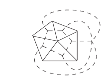
Such duals can be defined only for planar graphs.

To say that a Feynman diagram $G$ is (non-)planar, one defines the adjoint diagram $G^{*}$ (Fig. 2). It is constructed from $G$ by attaching all external lines to an auxiliary vertex [3].

Figure 2: A Feynman diagram (left) and its adjoint (right)

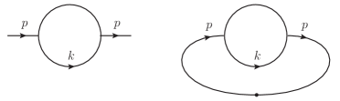
We say that a Feynman diagram $G$ is planar iff $G^{*}$ is planar.

2 Method I

Let $G$ be a connected $l-$loop Feynman diagram, $\{p_{1},...,p_{m}\}$ be the set of external momenta, $\{e_{1},...,e_{n}\}$ be the set of edges in $G$ (neglecting external lines), $\{k_{1},...,k_{n}\}$ be the set of corresponding momentum flows in $G$ and $\{v_{1},...,v_{r}\}$ be the set of vertices in $G$. Then there holds [5]

$$r=n-l+1.$$ (1)

Hence given the number of edges (flows) and loops, the number of vertices $r$ can be derived from (1). After introducing Feynman parameters $x_{1},...,x_{n}$, one defines the Laplacian matrix $L$ of a graph $G$ as a $r\times r$ matrix with entries

$$L_{ij}=\left\{\begin{array}[]{c l}\sum\limits_{k=1}^{n}x_{k}&\mbox{if }i=j,\mbox{ }e_{k}\mbox{ is attached to }v_{i},\mbox{ }e_{k}\mbox{ is not a self-loop,}\\ -\sum\limits_{k=1}^{n}x_{k}&\mbox{if }i\neq j,\mbox{ }e_{k}\mbox{ connects }v_{i},v_{j}.\end{array}\right.$$ (4)

Elements of $L$ are calculated in a few steps. Diagonal elements $L_{ii}$ are obtained by deciding which Feynman parameters $x_{k}$ are attached to $v_{i}$. Vertices are divided into external (attached to external lines) and internal ones. Note that only triple and quartic (i.e. of degree 3 and 4) vertices are allowed. Thus the conditions are of the form

$$\mbox{(for external vertices) }\pm k_{a}\pm k_{b}=\pm p_{e}\mbox{ or }\pm k_{a}\pm k_{b}\pm k_{c}=\pm p_{e},$$

$$\mbox{(for internal vertices) }\pm k_{a}\pm k_{b}=\pm k_{c}\mbox{ or }\pm k_{a}\pm k_{b}\pm k_{c}=\pm k_{d},$$

where $a,b,c,d\in\{1,...,n\}$, $e\in\{1,...,m\}$. The flows that fulfill the above relations contribute to diagonal elements of $L$. Furthermore, off-diagonal elements $L_{ij}$ are obtained by deciding Feynman parameters $x_{k}$ that connect vertices $v_{i}$, $v_{j}$. Observe that such $x_{k}$’s have to be both in $L_{ii}$ and $L_{jj}$, thus the intersection of elements in $L_{ii}$ and $L_{jj}$ is non-empty and gives exactly these $x_{k}$’s. In the case of many edges connecting $v_{i}$, $v_{j}$, they shrink to one edge, thus giving exactly one $x_{k}$ (hence $\sum x_{k}\rightarrow x_{k}$).
In order to obtain a more familiar form of $L$, understandable to Mathematica software [6], redefine $L$ by

$$L_{ij}=\left\{\begin{array}[]{c l}\mathrm{deg}\left(v_{i}\right)&\mbox{if }i=j,\\ -1&\mbox{if }i\neq j\mbox{ and }v_{i},v_{j}\mbox{ are adjacent},\end{array}\right.$$

where $\mathrm{deg}\left(v_{i}\right)$ is the degree of $v_{i}$. The above definition is derived from (4) by substituting $x_{k}\rightarrow 1$. Then $L$ can be written as

$$L=D-A,$$ (5)

where $D=\mathrm{diag}\left(\mathrm{deg}\left(v_{1}\right),...,\mathrm{deg}\left(v_{r}\right)\right)$ is a degree matrix and $A$ is the adjacency matrix given by

$$A_{ij}=\left\{\begin{array}[]{c l}1&\mbox{if }i\neq j\mbox{ and }v_{i},v_{j}\mbox{ are adjacent},\\ 0&\mbox{otherwise}.\end{array}\right.$$

The final part of the algorithm is to create the adjoint diagram $G^{*}$. The Laplacian matrix $L^{*}$ of $G^{*}$ is build upon $L$ by extending it by one row and one column corresponding to $v_{r+1}$. Clearly $\mathrm{deg}\left(v_{r+1}\right)=m$ and extra 1’s appear in the $\left(r+1\right)^{th}$ column and $\left(r+1\right)^{th}$ row at the elements corresponding to external vertices. Thus, from (5) the adjacency matrix $A^{*}=D^{*}-L^{*}$ is obtained. Eventually, given $A^{*}$, the function PlanarQ of the Mathematica package Combinatorica yields the answer for the question of planarity of a Feynman diagram $G$. Additionally, in [2] there was made a remark that it is possible to draw a diagram upon the set of denominators. In fact, given the matrix $A^{*}$ it is possible to draw a given diagram with Mathematica by using the function AdjacencyGraph. Instructive examples for planarity recognition using the described algorithm are given in [7].

3 Method II

Let $G$ be a connected $l-$loop Feynman diagram, $\{p_{1},...,p_{m}\}$ be the set of external momenta, $\{k_{1},...,k_{n}\}$ be the set of corresponding momentum flows in $G$. Dual variables $\{x_{1},\ldots,x_{m}\}$ are defined by (see e.g. [4])

$$p_{1}=x_{1}-x_{m},\mbox{ }p_{2}=x_{2}-x_{1},\mbox{ }\ldots\mbox{ },\mbox{ }p_{m}=x_{m}-x_{m-1}.$$ (6)

Then by introducing rules of the form $k_{i}\rightarrow x_{j}\pm x_{l}$ all momenta are substituted by dual variables and one obtains the following criterion: A Feynman diagram is planar iff it is possible to write all propagators (including external momenta) in the form $x_{i}\pm x_{l}$. Let us present two examples.

1. Let $G$ be a simple box diagram with four external lines $\{p_{1},\ldots,p_{4}\}$ and a loop momentum $k$. The amplitude is proportional to the integral

   $$\int\frac{\mathrm{d}^{4}k}{k^{2}\left(k-p_{1}\right)^{2}\left(k-p_{1}-p_{2}\right)^{2}\left(k-p_{1}-p_{2}-p_{3}\right)^{2}}.$$ (7)

   Introduce dual variables according to (6).

   

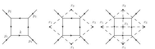
   Figure 3: A box diagram, external dual variables and dual graph, respectively

   Note that external momenta correspond to crossing of external lines and lines between corresponding dual variables (Fig. 3). The integral is now of the form

   $$\int\frac{\mathrm{d}^{4}k}{k^{2}\left(k-x_{1}+x_{4}\right)^{2}\left(k-x_{2}+x_{4}\right)^{2}\left(k-x_{3}+x_{4}\right)^{2}}.$$ (8)

   Observe that substitution $k\rightarrow x_{5}-x_{4}$ gives a conformal invariant object

   $$\int\frac{\mathrm{d}^{4}x_{5}}{\left(x_{5}-x_{4}\right)^{2}\left(x_{5}-x_{1}\right)^{2}\left(x_{5}-x_{2}\right)^{2}\left(x_{5}-x_{3}\right)^{2}}.$$ (9)

2. Let $G$ be a non-planar double box with

   $$\int\frac{\mathrm{d}^{4}k_{1}\mathrm{d}^{4}k_{2}}{k_{1}^{2}\left(k_{1}-p_{2}\right)^{2}\left(k_{1}-p_{1}-p_{2}\right)^{2}k_{2}^{2}\left(k_{2}+p_{3}\right)^{2}\left(k_{1}-k_{2}\right)^{2}\left(k_{1}-k_{2}+p_{4}\right)^{2}}$$ (10)

   and introduce dual variables again (Fig. 4).

   

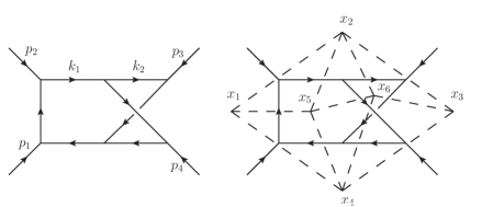
   Figure 4: Non-planar double box (left) and its dual variables (right)

   Obviously, since the diagram is non-planar, it does not have a dual. Note that after transforming momenta to dual variables, one of the possible forms of the integral is

   $$\int\frac{\mathrm{d}^{4}x_{5}\mathrm{d}^{4}x_{6}}{\left(x_{5}+x_{2}\right)^{2}\left(x_{5}+x_{1}\right)^{2}\cdot\ldots\cdot\left(x_{6}+x_{5}-x_{3}+x_{4}\right)^{2}}.$$ (11)

Non-planarity is encoded in the element $x_{6}+x_{5}-x_{3}+x_{4}$, that breaks the conformal invariance. Thus there is a strict correspondence between dual diagrams and dual variables, hence another planarity criterion for Feynman diagrams is established. Instructive examples for planarity recognition using described algorithm are given in [7].

4 Non-planar diagrams and dual variables

Figure 5: Three-loop non-planar self-energy (left) and its embedding on a torus (right)

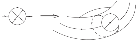
Observe that it is possible to planarize a non-planar diagram by embedding it on a surface with genus higher than 0. Actually, the minimal genus of a surface where the given diagram $G$ is planar is called the genus of $G$. Let us give an example. Let a three-loop non-planar self-energy be embedded on a torus. Then there is no crossing of diagram lines, hence the diagram is planar on the torus (Fig. 5). It is then possible to find its dual diagram and corresponding dual variables. Unfortunately, such an embedding sets the number of faces too small to give a proper interpretation of momenta by dual variables. It can be easily calculated by Euler’s formula that

$$\chi=v-e+f=2-2g=2-2\cdot 1=0\longrightarrow f=0-6+9=3,$$

where $\chi$ — Euler characteristics, $v$ — number of vertices, $e$ — number of edges, $f$ — number of faces (dual variables), $g$ — genus of a graph (surface). Thus there are only three dual variables $x_{1}$, $x_{2}$, $x_{3}$ available, in contrast to five momenta $p$, $-p$, $k_{1}$, $k_{2}$, $k_{3}$. Hence, although the non-planar diagram is planarized, it is not possible to define appropriate dual variables, since two momenta are absorbed by torus generators.

References

- [1] J. Gluza, K. Kajda, T. Riemann, Comput. Phys. Commun. 177 (2007) 879; J. Gluza, K. Kajda, T. Riemann and V. Yundin, Nucl. Phys. Proc. Suppl. 205 (2010) 147; ibid. Eur. Phys. J. C 71 (2011) 1516.
- [2] R. N. Lee, arXiv:1212.2685 [hep-ph].
- [3] N. Nakanishi, “Graph Theory and Feynman Integrals” (Routledge 1971).
- [4] J. Arkani-Hamed et al., JHEP 1206 (2012) 125.
- [5] C. Bogner and S. Weinzierl, Int. J. Mod. Phys. A25 (2010) 2585.
- [6] Wolfram Research, Inc., Mathematica, Champaign, IL (2010).
-
[7]
Katowice, webpage http://prac.us.edu.pl/gluza/ambre;
DESY, webpage http://www-zeuthen.desy.de/theory/research/CAS.html.