Learning rates of $l^{q}$ coefficient regularization learning with Gaussian kernel

Abstract

Regularization is a well recognized powerful strategy to improve the performance of a learning machine and $l^{q}$ regularization schemes with $0<q<\infty$ are central in use. It is known that different $q$ leads to different properties of the deduced estimators, say, $l^{2}$ regularization leads to smooth estimators while $l^{1}$ regularization leads to sparse estimators. Then, how does the generalization capabilities of $l^{q}$ regularization learning vary with $q$? In this paper, we study this problem in the framework of statistical learning theory and show that implementing $l^{q}$ coefficient regularization schemes in the sample dependent hypothesis space associated with Gaussian kernel can attain the same almost optimal learning rates for all $0<q<\infty$. That is, the upper and lower bounds of learning rates for $l^{q}$ regularization learning are asymptotically identical for all $0<q<\infty$. Our finding tentatively reveals that, in some modeling contexts, the choice of $q$ might not have a strong impact with respect to the generalization capability. From this perspective, $q$ can be arbitrarily specified, or specified merely by other no generalization criteria like smoothness, computational complexity, sparsity, etc..

I Introduction

Many scientific questions boil down to learning an underlying rule from finitely many input-output samples. Learning means synthesizing a function that can represent or approximate the underlying rule based on the samples. A learning system is normally developed for tackling such a supervised learning problem. Generally speaking, a learning system should comprise a hypothesis space, an optimization strategy and a learning algorithm. The hypothesis space is a family of parameterized functions that regulate the forms and properties of the estimator to be found. The optimization strategy depicts the sense in which the estimator is defined, and the learning algorithm is an inference process to yield the objective estimator. A central question of learning is and will always be: how well does the synthesized function generalize to reflect the reality that the given “examples” purport to show us.

A recent trend in supervised learning is to utilize the kernel approach, which takes a reproducing kernel Hilbert space (RKHS) [Cucker and Smale,2001] associated with a positive definite kernel as the hypothesis space. RKHS is a Hilbert space of functions in which the pointwise evaluation is a continuous linear functional. This property makes the sampling stable and effective, since the samples available for learning are commonly modeled by point evaluations of the unknown target function. Consequently, various learning schemes based on RKHS such as the regularized least squares (RLS) [Cucker and Smale,2001, 27, 22] and support vector machine (SVM) [15, 20] have triggered enormous research activities in the last decade. From the point of view of statistics, the kernel approach is proved to possess perfect learning capabilities [27, 22]. From the perspective of implementation, however, kernel methods can be attributed to such a procedure: to deduce an estimator by using the linear combination of finitely many functions, one firstly tackles the problem in an infinitely dimensional space and then reduces the dimension by utilizing a certain optimization technique. Obviously, the infinite dimensional assumption of the hypothesis space brings many difficulties to the implementation and computation in practice.

This phenomenon was firstly observed in [28], where Wu and Zhou suggested the use of the sample dependent hypothesis space (SDHS) directly to construct the estimators. From the so-called representation theorem in learning theory [Cucker and Smale,2001], the learning procedure in RKHS can be converted into such a problem, whose hypothesis space can be expressed as a linear combination of the kernel functions evaluated at the sample points with finitely many coefficients. Thus, it implies that the generalization capabilities of learning in SDHS are not worse than those of learning in RKHS in certain a sense. Furthermore, as SDHS is an $m$-dimensional linear space, various optimization strategies such as the coefficient-based regularization strategies [16, 28] and greedy-type schemes [Barron et al.,2008, 11] can be applied to construct the estimator.

In this paper, we consider the general coefficient-based regularization strategies in SDHS. Let

$$\mathcal{H}_{K,{\bf z}}:=\left\{\sum_{i=1}^{m}a_{i}K_{x_{i}}:a_{i}\in\mathbf{R}\right\}$$

be a SDHS, where $K_{t}(\cdot)=K(\cdot,t)$ and $K(\cdot,\cdot)$ is a positive definite kernel. The coefficient-based $l^{q}$ regularization strategy ($l^{q}$ regularizer) takes the form of

$$f_{{\bf z},\lambda,q}=\arg\min_{f\in\mathcal{H}_{K,{\bf z}}}\left\{\frac{1}{m}\sum_{i=1}^{m}(f(x_{i})-y_{i})^{2}+\lambda\Omega^{q}_{\bf z}(f)\right\},$$ (1)

where $\lambda=\lambda(m,q)>0$ is the regularization parameter and $\Omega_{\bf z}^{q}(f)$ $(0<q<\infty)$ is defined by

$$\Omega^{q}_{\bf z}(f)=\sum_{i=1}^{m}|a_{i}|^{q}\ \mbox{when}\ f=\sum_{i=1}^{m}a_{i}K_{x_{i}}\in\mathcal{H}_{K,{\bf z}}.$$

I-A Problem setting

In practice, the choice of $q$ in (1) is critical, since it embodies the properties of the anticipated estimators such as sparsity and smoothness, and also takes some other perspectives such as complexity and generalization capability into consideration. For example, for $l^{2}$ regularizer, the solution to (1) is the same as the solution to the regularized least squares (RLS) algorithm in RKHS [Cucker and Smale,2001]

$$f_{{\bf z},\lambda}=\arg\min_{f\in H_{K}}\left\{\frac{1}{m}\sum_{i=1}^{m}(f(x_{i})-y_{i})^{2}+\lambda\|f\|^{2}_{H_{K}}\right\},$$ (2)

where $H_{K}$ is the RKHS associated with the kernel $K$. Furthermore, the solution can be analytically represented by the kernel function [Cucker and Zhou,2007]. The obtained solution, however, is smooth but not sparse, i.e., the nonzero coefficients of the solution are potentially as many as the sampling points if no special treatment is taken. Thus, $l^{2}$ regularizer is a good smooth regularizer but not a sparse one. For $0<q<1$, there are many algorithms such as the iteratively reweighted least squares algorithm [2] and iterative half thresholding algorithm [31] to obtain a sparse approximation of the target function. However, all of these algorithms suffer from the local minimum problem due to the non-convex natures. For $q=1$, many algorithms exist, say, iterative soft thresholding algorithm [1], LASSO [8, 24] and iteratively reweighted least square algorithm [2], to yield sparse estimators of the target function. However, as far as the sparsity is concerned, the $l^{1}$ regularizer is somewhat worse than the $l^{q}$ $(0<q<1)$ regularizer, while as far as the training speed is concerned, the $l^{1}$ regularizer is in turn slower than that of the $l^{2}$ regularizer. Thus, we can see that, different choices of $q$ may deduce estimators with different forms, properties, and attributions. Since the study of generalization capabilities lies in the center of learning theory, we would like to ask the following question: what about the generalization capabilities of the $l^{q}$ regularization schemes (1) for $0<q<\infty$?

Answering the above question is of great importance, since it uncovers the role of the penalty term in the regularization learning, which then further underlies the learning strategies. However, it is known that the approximation capability of SDHS depends heavily on the choice of the kernel, it is therefore almost impossible to give a general answer to the above question independent of kernel functions. In this paper, we aim to provide an answer to the above question when the widely used Gaussian kernel is utilized.

I-B Related work and our contribution

There exists a huge number of theoretical analysis of kernel methods, many of which are treated in [Cucker and Smale,2001, Cucker and Zhou,2007, 5, Caponnetto and DeVito,2007, 20, 15] and references therein. This means that various results on the learning rate of the algorithm (2) are given. The recent work [13] suggested that the penalty $\|f\|^{2}_{H_{K}}$ may not be the optimal choice from a statistical point of view, that is, the RLS strategy may have a design flaw. There may be an appropriate choice of $q$ in the following optimization strategy

$$f^{q}_{{\bf z},\lambda}=\arg\min_{f\in H_{K}}\left\{\frac{1}{m}\sum_{i=1}^{m}(f(x_{i})-y_{i})^{2}+\lambda\|f\|^{q}_{H_{K}}\right\}$$ (3)

such that the performance of learning process can be improved. To this end, Steinwart et al. [22] derived a $q$-independent optimal learning rate of (3) in the minmax sense. Therefore, they concluded that the RLS strategy (2) has no advantages or disadvantages compared to other values of $q$ in (3) from the viewpoint of learning theory. However, even without such a result, it is unclear how to solve (3) when $q\neq 2$. That is, $q=2$ is currently the only feasible case, which in turn makes RLS strategy the method of choice.

Differently, $l^{q}$ coefficient regularization strategy (1) is solvable for arbitrary $0<q<\infty$. Thus, studying the learning performance of the strategy (1) with different $q$ is more interesting. Based on a series of work as [6, 16, 23, 25, 28, 30], we have shown that there is a positive definite kernel such that the learning rate of the corresponding $l^{q}$ regularizer is independent of $q$ in the previous paper [10]. However, the problem is that the kernel constructed in [10] can not be easily formulated in practice. Thus, seeking kernels that possess the similar property and can be easily implemented is worth of investigation.

Fortunately, we show in the present paper that the well known Gaussian kernel possesses similar property, that is, as far as the learning rate is concerned, all $l^{q}$ regularization schemes (1) associated with the Gaussian kernel for $0<q<\infty$ can realize the same almost optimal theoretical rates. That is to say, the influence of $q$ on the learning rates of the learning schemes (1) with Gaussian kernel is negligible. Here, we emphasize that our conclusion is based on the understanding of attaining the same almost optimal learning rate by appropriately tuning the regularization parameter $\lambda$. Thus, in applications, $q$ can be arbitrarily specified, or specified merely by other no generalization criteria (like complexity, sparsity, etc.).

I-C Organization

The reminder of the paper is organized as follows. In Section 2, after reviewing some basic conceptions of statistical learning theory, we give the main results of this paper, that is, the learning rates of $l^{q}$ $(0<q<\infty)$ regularizers associated with Gaussian kernel are provided. In section 3, the proof of the main result is given.

II Generalization capabilities $l^{q}$ coefficient regularization learning

II-A A fast review of statistical learning theory

Let $M>0$, $X\subseteq\mathbf{R}^{d}$ be an input space and $Y\subseteq[-M,M]$ be an output space. Let ${\bf z}=(x_{i},y_{i})_{i=1}^{m}$ be a random sample set with a finite size $m\in\mathbf{N}$, drawn independently and identically according to an unknown distribution $\rho$ on $Z:=X\times Y$, which admits the decomposition

$$\rho(x,y)=\rho_{X}(x)\rho(y|x).$$

Suppose further that $f:X\rightarrow Y$ is a function that one uses to model the correspondence between $x$ and $y$, as induced by $\rho$. A natural measurement of the error incurred by using $f$ of this purpose is the generalization error, defined by

$$\mathcal{E}(f):=\int_{Z}(f(x)-y)^{2}d\rho,$$

which is minimized by the regression function [Cucker and Smale,2001], defined by

$$f_{\rho}(x):=\int_{Y}yd\rho(y|x).$$

However, we do not know this ideal minimizer $f_{\rho}$ due to $\rho$ is unknown. Instead, we can turn to the random examples sampled according to $\rho$.

Let $L^{2}_{\rho_{{}_{X}}}$ be the Hilbert space of $\rho_{X}$ square integrable function defined on $X$, with norm denoted by $\|\cdot\|_{\rho}.$ Under the assumption $f_{\rho}\in L^{2}_{\rho_{{}_{X}}}$, it is known that, for every $f\in L^{2}_{\rho_{X}}$, there holds

$$\mathcal{E}(f)-\mathcal{E}(f_{\rho})=\|f-f_{\rho}\|^{2}_{\rho}.$$ (4)

The task of the least squares regression problem is then to construct function $f_{\bf z}$ that approximates $f_{\rho}$, in the sense of norm $\|\cdot\|_{\rho}$, using the finitely many samples ${\bf z}$.

II-B Learning rate analysis

Let

$$G_{\sigma}(x,x^{\prime}):=G_{\sigma}(x-x^{\prime}):=\exp\{-\|x-x^{\prime}\|_{2}^{2}/\sigma^{2}\},\ x,x^{\prime}\in X$$

be the Gaussian kernel, where $\sigma>0$ is called the width of $G_{\sigma}$. The SDHS associated with $G_{\sigma}(\cdot,\cdot)$ is then defined by

$$\mathcal{G}_{\sigma,{\bf z}}:=\left\{\sum_{i=1}^{m}a_{i}G_{\sigma}(x_{i},\cdot):a_{i}\in\mathbf{R}\right\}.$$

We are concerned with the following $l^{q}$ coefficient-based regularization strategy

$$f_{{\bf z},\lambda,q}=\arg\min_{f\in\mathcal{G}_{\sigma,{\bf z}}}\left\{\frac{1}{m}\sum_{i=1}^{m}(f(x_{i})-y_{i})^{2}+\lambda\sum_{i=1}^{m}|a_{i}|^{q}\right\},$$ (5)

where $f(x)=\sum_{i=1}^{m}a_{i}G_{\sigma}(x_{i},x)$. The main purpose of this paper is to derive the optimal bound of the following generalization error

$$\mathcal{E}(f_{{\bf z},\lambda,q})-\mathcal{E}(f_{\rho})=\|f_{{\bf z},\lambda,q}-f_{\rho}\|^{2}_{\rho}$$ (6)

for all $0<q<\infty$.

Generally, it is impossible to obtain a nontrivial rate of convergence result of (6) without imposing strong restrictions on $\rho$ [7, Chapter 3] . Then a large portion of learning theory proceeds under the condition that $f_{\rho}$ is in a known set $\Theta$. A typical choice of $\Theta$ is a set of compact sets, which are determined by some smoothness conditions [4]. Such a choice of $\Theta$ is also adopted in our analysis. Let $X=\mathbf{I}^{d}:=[0,1]^{d}$, $c_{0}$ be a positive constant, $v\in(0,1]$, and $r=u+v$ for some $u\in\mathbf{N}_{0}:=\{0\}\cup\mathbf{N}$. A function $f:\mathbf{I}^{d}\rightarrow\mathbf{R}$ is said to be $(r,c_{0})$-smooth if for every $\alpha=(\alpha_{1},\cdots,\alpha_{d}),\alpha_{i}\in N_{0},$ $\sum_{j=1}^{d}\alpha_{j}=u$, the partial derivatives $\frac{\partial^{u}f}{\partial x{{}_{1}}^{\alpha_{1}}...\partial x{{}_{d}}^{\alpha_{d}}}$ exist and satisfy

$$\left|\frac{\partial^{u}f}{\partial x{{}_{1}}^{\alpha_{1}}\cdots\partial x{{}_{d}}^{\alpha_{d}}}(x)-\frac{\partial^{u}f}{\partial x{{}_{1}}^{\alpha_{1}}\cdots\partial x{{}_{d}}^{\alpha_{d}}}(z)\right|\leq c_{0}\|x-z\|^{v}_{2}.$$

Denote by $\mathcal{F}^{(r,c_{0})}$ the set of all $(r,c_{0})$-smooth functions. In our analysis, we assume the prior information $f_{\rho}\in\mathcal{F}^{(r,c_{0})}$ is known.

Let $\pi_{M}t$ denote the clipped value of $t$ at $\pm M$, that is, $\pi_{M}t:=\min\{M,|t|\}\mbox{sgn}t$, where $\mbox{sgn}t$ represents the signum function of $t$. Then it is obvious [7, 22, 35] that for all $t\in\mathbf{R}$ and $y\in[-M,M]$ there holds

$$\mathcal{E}(\pi_{M}f_{{\bf z},\lambda,q})-\mathcal{E}(f_{\rho})\leq\mathcal{E}(f_{{\bf z},\lambda,q})-\mathcal{E}(f_{\rho}).$$

The following theorem shows the learning capability of the leaning strategy (5) for arbitrary $0<q<\infty$.

Theorem 1

Let $r>0$, $c_{0}>0$, $\delta\in(0,1)$, $0<q<\infty$, $f_{\rho}\in\mathcal{F}^{r,c_{0}}$, and $f_{{\bf z},\lambda,q}$ be defined as in (5). If $\sigma=m^{-\frac{1}{2r+d}}$, and

$$\lambda=\left\{\begin{array}[]{cc}M^{2}m^{\frac{-12r-6d+2rq+qd}{4r+2d}},&0<q\leq 2.\\ M^{2}m^{-\frac{4r+2d}{2r+d}},&q>2,\end{array}\right.$$

then, for arbitrary $\varepsilon>0$, with probability at least $1-\delta$, there holds

$$\mathcal{E}(\pi_{M}f_{{\bf z},\lambda,q})-\mathcal{E}(f_{\rho})\leq C\log\frac{4}{\delta}m^{-\frac{2r-\varepsilon}{2r+d}},$$ (7)

where $C$ is a constant depending only on $d$, $r$, $c_{0}$, $q$ and $M$.

II-C Remarks

In this subsection, we give certain explanations and remarks of Theorem 1. We depict it into four directions: remarks on the learning rate, the choice of the width of Gaussian kernel, the role of the regularization parameter, and the relationship between $q$ and the generalization capability.

II-C1 Learning rate analysis

It can be found in [7] and [4] that if we only know $f_{\rho}\in\mathcal{F}^{r,c_{0}}$, then the learning rates of all learning strategies based on $m$ samples can not be faster than $m^{-\frac{2r}{2r+d}}.$ More specifically, let $\mathcal{M}(\mathcal{F}^{r,c_{0}})$ be the class of all Borel measures $\rho$ on $Z$ such that $f_{\rho}\in\mathcal{F}^{r,c_{0}}$. We enter into a competition over all estimators $\mathcal{A}_{m}:{\bf z}\rightarrow f_{\bf z}$ and define

$$e_{m}(\mathcal{F}^{r,c_{0}}):=\inf_{\mathcal{A}_{m}}\sup_{\rho\in\mathcal{M}(\mathcal{F}^{r,c_{0}})}E_{\rho^{m}}(\|f_{\rho}-f_{\bf z}\|^{2}_{\rho}).$$

It is easy to see that $e_{m}(\mathcal{F}^{r,c_{0}})$ quantitively measures the quality of $f_{\bf z}$. Then it can be found in [7, Chapter 3] or [4] that

$$e_{m}(\mathcal{F}^{r,c_{0}})\geq Cm^{-\frac{2r}{2r+d}},\ m=1,2,\dots,$$ (8)

where $C$ is a constant depending only on $M$, $d$, $c_{0}$ and $r$.

Modulo the arbitrary small positive number $\varepsilon$, the established learning rate (7) is asymptotically optimal in a minmax sense. If we notice the identity:

$$\mathbf{E}_{\rho^{m}}(\mathcal{E}(f_{\rho})-\mathcal{E}(f_{{\bf z},\lambda,q}))=\int_{0}^{\infty}\mathbf{P}_{\rho^{m}}\{\mathcal{E}(f_{\rho})-\mathcal{E}(f_{{\bf z},\lambda,q})>\varepsilon\}d\varepsilon.$$

then there holds

$$C_{1}m^{-\frac{2r}{2r+d}}\leq e_{m}(\mathcal{F}^{r,c_{0}})\leq\sup_{f_{\rho}\in\mathcal{F}^{r,c_{0}}}\mathbf{E}_{\rho^{m}}\left\{\mathcal{E}(\pi_{M}f_{{\bf z},\lambda,q})-\mathcal{E}(f_{\rho})\right\}\leq C_{2}m^{-\frac{2r}{2r+d}+\varepsilon},$$ (9)

where $C_{1}$ and $C_{2}$ are constants depending only on $r$, $c_{0}$, $M$ and $d$.

Due to (9), we know that the learning strategy (5) is almost the optimal method if the smoothness information of $f_{\rho}$ is known. It should be highlighted that the above optimality is given in the background of the worst case analysis. That is, for a concrete $f_{\rho}$, the learning rate of the strategy (5) may be much faster than $m^{-\frac{2r}{2r+d}}$. For example, if the concrete $f_{\rho}\in\mathcal{F}^{2r,c_{0}}\subset\mathcal{F}^{r,c_{0}}$, then the learning rate of (5) can achieve to $m^{-\frac{4r}{4r+d}+\varepsilon}$. Summarily, the conception of optimal learning rate is based on $\mathcal{F}^{r,c_{0}}$ rather than a fixed regression functions.

II-C2 Choice of the width

The width of Gaussian kernel determines both approximation capability and complexity of the corresponding RKHS, and thus plays a crucial role in the learning process. Admittedly, as a function of $\sigma$, the complexity of the Gaussian RKHS is monotonically decreasing. Thus, due to the so-called bias and variance problem in learning theory [Cucker and Zhou,2007], there exists an optimal choice of $\sigma$ for the Gaussian kernel method. Since SDHS is essentially an $m$-dimensional linear space and the Gaussian RKHS is an infinite space for arbitrary $\sigma$ (kernel width) [14], the complexity of the Gaussian SDHS may be smaller than the Gaussian RKHS at the first glance. Hence, there naturally arises the following question: does the optimal $\sigma$ of the Gaussian SDHS learning coincide with that of the Gaussian RKHS learning? Theorem 1 together with [5, Corollary 3.2] demonstrate that the optimal widths of the above two strategies are asymptomatically identical. That is, if the smooth information of the regression function is known, then the optimal choices of $\sigma$ of both learning strategies (5) and (2) are the same. The above phenomenon can be explained as follows. Let $B_{H_{\sigma}}$ be the unit ball of the Gaussian RKHS and $B_{2}:=\left\{f\in G_{\sigma,{\bf z}}:\frac{1}{n}\sum_{i=1}^{n}|f(x_{i})|^{2}\leq 1\right\}$ be the $l^{2}$ empirical ball. Denote by $\mathcal{N}_{2}(B_{H_{\sigma}},\varepsilon)$ the $l_{2}$-empirical covering number [16], whose definition can be found in the descriptions above Lemma 5 in the present paper. Then it can be found in [20, Theorem 2.1] that for any $\varepsilon>0$, there holds

$$\log\mathcal{N}_{2}(B_{H_{\sigma}},\varepsilon)\leq C_{p,\mu,d}\sigma^{(p/2-1)(1+\mu)d}\varepsilon^{-p},$$ (10)

where $p$ is an arbitrary real number in $(0,2]$ and $\mu$ is an arbitrary positive number. For the Gaussian SDHS, $\mathcal{G}_{\sigma,{\bf z}}$, on one hand, we can use the fact that $\mathcal{G}_{\sigma,{\bf z}}\subset H_{\sigma}$ and deduce

$$\log\mathcal{N}_{2}(B_{2},\varepsilon)\leq C^{\prime}_{p,\mu,d}\sigma^{(p/2-1)(1+\mu)d}\varepsilon^{-p},$$ (11)

where $C^{\prime}_{p,\mu,d}$ is a constant depending only on $p,\mu$ and $d$. On the other hand, it follows from [7, Lemma 9.3] that

$$\log\mathcal{N}_{2}(B_{2},\varepsilon)\leq C_{d}m\log\frac{4+\varepsilon}{\varepsilon}$$ (12)

where the finite-dimensional property of $\mathcal{G}_{\sigma,{\bf z}}$ is used. Therefore, it should be highlighted that the finite-dimensional property of $\mathcal{G}_{\sigma,{\bf z}}$ is used if

$$C_{d}m\log\frac{4+\varepsilon}{\varepsilon}\leq C^{\prime}_{p,\mu,d}\sigma^{(p/2-1)(1+\mu)d}\varepsilon^{-p},$$

which always implies that $\sigma$ is very small (may be smaller than $\frac{1}{m}$).

However, to deduce a good approximation capability of $\mathcal{G}_{\sigma,{\bf z}}$, it can be deduced from [12] that $\sigma$ can not be very small. Thus, we use (11) rather than (12) to describe the complexity of $\mathcal{G}_{\sigma,{\bf z}}$. Noting (10), when $\sigma$ is not very small (corresponding to $1/m$), the complexity of $\mathcal{G}_{\sigma,{\bf z}}$ asymptomatically equals to that of $H_{\sigma}$. Under this circumstance, recalling that the optimal widths of the learning strategies (2) and (5) may not be very small, the capacities of $\mathcal{G}_{\sigma,{\bf z}}$ and $H_{\sigma}$ are asymptomatically identical. Therefore, the optimal choice of $\sigma$ in (5) are the same as that in (2).

II-C3 Importance of the regularization term

We can address the regularized learning model as a collection of empirical minimization problems. Indeed, let $\mathcal{B}$ be the unit ball of a space related to the regularization term and consider the empirical minimization problem in $r\mathcal{B}$ for some $r>0$. As $r$ increases, the approximation error for $r\mathcal{B}$ decreases and its sample error increases. We can achieve a small total error by choosing the correct value of $r$ and performing empirical minimization in $r\mathcal{B}$ such that the approximation error and sample error are asymptomatically identical. The role of regularization term is to force the algorithm to choose the correct value of $r$ for empirical minimization [13] and then provides a method of solving the bias-variance problem. Therefore, the main role of the regularization term is to control the capacity of the hypothesis space.

Compared with the regularized least squares strategy (2), a consensus is that $l^{q}$ coefficient regularization schemes (5) may bring a certain additional interest such as the sparsity for suitable choice of $q$ [16]. However, it should be noticed that this assertion may not always be true.

There are usually two criteria to choose the regularization parameter in such a setting:

1. the approximation error should be as small as possible;

2. the sample error should be as small as possible.

Under the criterion (a), $\lambda$ should not be too large, while under the criterion (b), $\lambda$ can not be too small. As a consequence, there is an uncertainty principle in the choice of the optimal $\lambda$ for generalization. Moreover, if the sparsity of the estimator is needed, another criterion should be also taken into consideration, that is,

1. The sparsity of the estimator should be as sparse as possible.

The sparsity criterion (c) requires that $\lambda$ should be large enough, since the sparsity of the estimator monotonously decreases with respect to $\lambda$. It should be pointed out that the optimal $\lambda_{0}$ for generalization may be smaller than the smallest value of $\lambda$ to guarantee the sparsity. Therefore, to obtain the sparse estimator, the generalization capability may degrade in certain a sense. Summarily, $l^{q}$ coefficient regularization scheme may brings a certain additional attribution of the estimator without sacrificing the generalization capability but not always so. It may depend on the distribution $\rho$, the choice of $q$ and the samples. In a word, the $l^{q}$ coefficient regularization scheme (5) provides a possibility to bring other advantages without degrading the generalization capability. Therefore, it may outperform the classical kernel methods in certain a sense.

II-C4 $q$ and learning rate

Generally speaking, the generalization capability of $l^{q}$ regularization scheme (5) may depend on the width of Gaussian kernel, the regularization parameter $\lambda$, the behavior of priors, the size of samples $m$, and, obviously, the choice of $q$. While from Theorem 1 and (9), it has been demonstrated that the learning schemes defined by (5) can indeed achieve the asymptotically optimal rates for all choices of $q$. In other words, the choice of $q$ has no influence on the learning rate, which in turn means that $q$ should be chosen according to other non-generalization considerations such as the smoothness, sparsity, and computational complexity.

This assertion is not surprising if we cast $l^{q}$ regularization schemes (5) into the process of empirical minimization. From the above analysis, it is known that the width of Gaussian kernel depicts the complexity of the $l^{q}$ empirical unit ball and the regularization parameter describes the choice of the radius of the $l^{q}$ ball. It should be also pointed out that the choice of $q$ implies the route of the change in order to find the hypothesis space with the appropriate capacity. A regularization scheme can be regarded as the following process according to the bias and variance problem. One first chooses a large hypothesis space to guarantee the small approximation error, and then shrinks the capacity of the hypothesis space until the sample error and approximation error being asymptomatically identical. It can be found in Fig.1 that $l_{q}$ regularization schemes with different $q$ may possess different paths of shrinking, and then derive estimators with different attributions.

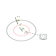
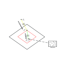
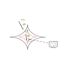
Figure 1: The above three figures show the routes of the change of $l^{2}$, $l^{1}$ and $l^{1/2}$ regularizers, respectively.

From Fig.1, it also shows that, by appropriately tuning the regularization (the radius of the $l^{q}$ empirical ball), we can always obtain $l^{q}$ regularizer estimators for all $0<q<\infty$ with the similar learning rates. In such a sense, it can be concluded that the learning rate of $l^{q}$ regularization learning is independent of the choice of $q$.

II-D Comparisons

In this subsection, we give many comparisons between Theorem 1 and the related work to show the novelty of our result. We divide the comparisons into the following three categories. At first, we illustrate the difference between learning in RKHS and SDHS associated with Gaussian kernel. Then we compare our result with the existing results on coefficient-based regularization in SDHS. Finally, we refer certain papers concerning the choice of regularization exponent $q$ and show the novelty of our result.

II-D1 Learning in RKHS and SDHS with Gaussian kernel

Kernel methods with Gaussian kernels are one of the classes of the standard and state-of-the-art learning strategies. Therefore, the corresponding properties such as the covering numbers, RKHS norms, formats of the elements in the RKHS, associated with Gaussian kernels were studied in [21, 14, 34, 19]. Based on these analyses, the learning capabilities of Gaussian kernel learning were thoroughly revealed in [5, 32, 9, 20, 29] and references therein. For classification, [20] showed that the learning rates for support vector machines with hinge loss and Gaussian kernel can attain the order of $m^{-1}$. For regression, it was shown in [5] that the regularized least squares algorithm with Gaussian kernel can achieve the almost optimal learning rate if the smoothness information of the regression function is given.

However, the learning capability of the coefficient-based regularization scheme (5) remains open. It should be stressed that the roles of regularization terms in (5) and (2) are distinct even though the solutions to these two schemes are identical for $q=2$. More specifically, without the regularization term, there are infinite many solutions to the least squares problem in the Gaussian RKHS. In order to obtain an expected and unique solution, we should impose a certain structure upon the solution, which can be achieved via introducing a specified regularization term. Therefore, the regularized least squares algorithm (2) can be regarded as a structural risk minimization strategy since it chooses a solution with the simplest structure among the infinite many solutions. However, due to the positive definiteness of the Gaussian kernel, there is a unique solution to (5) with $\lambda=0$ and the role of regularization can be regarded to improve the generalization capability only. Summarily, the introduction of regularization in (2) can be regarded as a passive choice, while that in (5) is an active operation.

The above difference requires different technique to analyze the performance of strategy (5). Indeed, the most widely used method was proposed in [28]. Based on [26], [28] pointed out that the generalization error can be divided into three terms: approximation error, sample error and hypothesis space. Basically, the generalization error can be bounded via the following three steps:

1. Find an alternative estimator outside the SDHS to approximate the regression function;

2. Find an approximation of the alternative function in SDHS and deduce the hypothesis error;

3. Bound the sample error which describes the distance between the approximant in SDHS and the $l_{q}$ regularizer.

In this paper, we also employ this technique to analyze the performance of the learning strategy (5). Our result shows that, similar to the regularized least squares algorithm [5], $l^{q}$ coefficient-based regularization scheme (5) can also achieve the almost optimal learning rate if the smoothness information of the regression function is given.

II-D2 $l^{q}$ regularizer with fixed $q$

There have been several papers that focus on the generalization capability analysis of the $l^{q}$ regularization scheme (1). [28] was the first paper, to the best of our knowledge, to show a mathematical foundation of learning algorithms in SDHS. They claimed that the data dependent nature of the algorithm leads to an extra hypothesis error, which is essentially different form regularization schemes with sample independent hypothesis spaces (SIHSs). Based on this, the authors proposed a coefficient-based regularization strategy and conducted a theoretical analysis of the strategy by dividing the generalization error into approximation error, sample error and hypothesis error. Following their work, [30] derived a learning rate of $l^{1}$ regularizer via bounding the regularization error, sample error and hypothesis error, respectively. Their result was improved in [16] by adopting a concentration technique with $l^{2}$ empirical covering numbers to tackle the sample error. On the other hand, for $l^{q}$ $(1\leq q\leq 2)$ regularizers, [25] deduced an upper bound for the generalization error by using a different method to cope with the hypothesis error. Later, the learning rate of [25] was improved further in [6] by giving a sharper estimation of the sample error.

In all those researches, both spectrum assumption of the regression function $f_{\rho}$ and the concentration property of $\rho_{X}$ should be satisfied. Noting this, for $l^{2}$ regularizer, [23] conducted a generalization capability analysis for $l^{2}$ regularizer by using the spectrum assumption to the regression function only. For $l^{1}$ regularizer, by using a sophisticated functional analysis method, [33] and [18] built the regularized least squares algorithm on the reproducing kernel Banach space (RKBS), and proved that the regularized least squares algorithm in RKBS is equivalent to $l^{1}$ regularizer if the kernel satisfies some restricted conditions. Following this method, [17] deduced a similar learning rate for the $l^{1}$ regularizer and eliminated the concentration assumption on the marginal distribution .

To intrinsically characterize the generalization capability of a learning strategy, the essential generalization bound rather than the upper bound is desired, that is, we must deduce both the lower and upper bounds for the learning strategy and prove that the upper and lower bounds can be asymptotically identical. Under this circumstance, we can essentially deduce the learning capability of the learning scheme. All of the above results for $l^{q}$ regularizers with fixed $q$ were only concerned with the upper bound. Thus, it is generally difficult to reveal their essential learning capabilities. Nevertheless, as shown by Theorem 1, our established learning rate is essential. It can be found in (9) that if $f_{\rho}\in\mathcal{F}^{r,c_{0}}$, then the deduced learning rate cannot be improved.

II-D3 The choice of $q$

[Blanchard et al.,2008] is the first paper, to the best of our knowledge, that focuses on the choice of the optimal $q$ for the kernel method. Indeed, as far as the sample error is concerned, [Blanchard et al.,2008] pointed out that there is an optimal exponent $q\neq 2$ for support vector machine with hinge loss. Then, [13] found that this assertion also held for the regularized least square strategy (3). That is, as far as the sample error is concerned, regularized least squares may have a design flaw. However, in [22], Steinwart et al. derived a $q$-independent optimal learning rate of (3) in a minmax sense. Therefore, they concluded that the RLS algorithm (2) had no advantages or disadvantages compared with other values of $q$ in (3) from the statistical point of view.

Since $l^{q}$ coefficient regularization strategy (1) is solvable for arbitrary $0<q<\infty$, and different $q$ may derive different attributions of the estimator, studying the dependence between learning performance of learning strategy (1) and $q$ is more interesting. This topic was first studied in [10], where we have shown that there is a positive definite kernel such that the learning rate of the corresponding $l^{q}$ regularizer is independent of $q$. However, the kernel constructed in [10] can not be easily formulated in practice. Thus, we turn to study the dependency of the generalization capabilities and $q$ of $l^{q}$ regularization learning with the widely used Gaussian kernel. Fortunately, we find that the similar conclusion also holds for the Gaussian kernel, which is witnessed in Theorem 1 in this paper.

III Proof of Theorem 1.

III-A Error decomposition

For an arbitrary $u=(u_{1},\dots,u_{d})\in\mathbf{I}^{d}$, define $F^{(0)}_{\rho}(u)=f_{\rho}(u).$ To construct a function $F_{\rho}^{(1)}$ defined on $[-1,1]^{d}$, we can define

$$F_{\rho}^{(1)}(u_{1},\dots,u_{j-1},-u_{j},u_{j+1},\dots,u_{d})=F_{\rho}^{(0)}(u_{1},\dots,u_{j-1},u_{j},u_{j+1},\dots,u_{d})$$

for arbitrary $j=1,2,\dots,d$. Finally, for every $j=1,\dots,d$, we define

$$F_{\rho}(u_{1},u_{j-1},u_{j}+2,u_{j+1},\dots,u_{d})=F_{\rho}^{(1)}(u_{1},\dots,u_{j-1},u_{j},u_{j+1},\dots,u_{d}).$$

Therefore, we have constructed a function $F_{\rho}$ defined on $\mathbf{R}^{d}$. From the definition, it follows that $F_{\rho}$ is an even, continuous and periodic function with respect to arbitrary variable $u_{i},i=1,\dots,d$.

In order to give an error decomposition strategy for $\mathcal{E}(\pi_{M}f_{{\bf z},\lambda,q})-\mathcal{E}(f_{\rho})$, we should construct a function $f_{0}\in H_{K}$ as follows. Define

$$f_{0}(x):=K*F_{\rho}:=\int_{\mathbf{R}^{d}}K(x-u)F_{\rho}(u)du,\ x\in\mathbf{I}^{d},$$ (13)

where

$$K(x):=\sum_{j=1}^{r}\left({}^{r}_{j}\right)(-1)^{1-j}\frac{1}{j^{d}}\left(\frac{2}{\sigma^{2}\pi}\right)^{d/2}G_{\frac{j\sigma}{\sqrt{2}}}(x),$$

Denote by $\mathcal{H}_{\sigma}$ and $\|\cdot\|_{\sigma}$ the RKHS associated with $G_{\sigma}$ and its corresponding RKHS norm, respectively. To prove Theorem 1, the following error decomposition strategy is required.

Proposition 1

Let $f_{{\bf z},\lambda,q}$ and $f_{0}$ be defined as in (5) and (13), respectively. Then we have

$$\mathcal{E}(\pi_{M}f_{{\bf z},\lambda,q})-\mathcal{E}(f_{\rho}) \leq \mathcal{E}(f_{0})-\mathcal{E}(f_{\rho})+\frac{1}{m}\|f_{0}\|_{\sigma}^{2}$$

$$+ \left(\mathcal{E}_{\bf z}(\pi_{M}f_{{\bf z},\lambda,q})+\lambda\sum_{i=1}^{m}|a_{i}|^{q}\right)-\left(\mathcal{E}_{\bf z}(f_{0})+\frac{1}{m}\|f_{0}\|_{\sigma}^{2}\right)$$

$$+ \mathcal{E}_{\bf z}(f_{0})-\mathcal{E}(f_{0})+\mathcal{E}(\pi_{M}f_{{\bf z},\lambda,q})-\mathcal{E}_{\bf z}(\pi_{M}f_{{\bf z},\lambda,q}),$$

where $\mathcal{E}_{\bf z}(f)=\frac{1}{m}\sum_{i=1}^{m}(y_{i}-f(x_{i}))^{2}$.

Upon making the short hand notations

$$\mathcal{D}(m):=\mathcal{E}(f_{0})-\mathcal{E}(f_{\rho})+\frac{1}{m}\|f_{0}\|_{\sigma}^{2},$$

$$\mathcal{S}(m,\lambda,q):=\mathcal{E}_{\bf z}(f_{0})-\mathcal{E}(f_{0})+\mathcal{E}(\pi_{M}f_{{\bf z},\lambda,q})-\mathcal{E}_{\bf z}(\pi_{M}f_{{\bf z},\lambda,q}),$$

and

$$\mathcal{P}(m,\lambda,q):=\left(\mathcal{E}_{\bf z}(\pi_{M}f_{{\bf z},\lambda,q})+\lambda\sum_{i=1}^{m}|a_{i}|^{q}\right)-\left(\mathcal{E}_{\bf z}(f_{0})+\frac{1}{m}\|f_{0}\|_{\sigma}^{2}\right)$$

for the approximation error, sample error and hypothesis error, respectively, then we have

$$\mathcal{E}(\pi_{M}f_{{\bf z},\lambda,q})-\mathcal{E}(f_{\rho})\leq\mathcal{D}(m)+\mathcal{S}(m,\lambda,q)+\mathcal{P}(m,\lambda,q).$$ (14)

III-B Approximation error estimation

Let $A\subseteq\mathbf{R}^{d}$. Denote by $C(A)$ the space of continuous functions defined on $A$ endowed with norm $\|\cdot\|_{A}$. Denote by

$$\omega_{r}(f,t,A)=\sup_{\|{\bf h}\|_{2}\leq t}\|\Delta_{{\bf h},A}^{r}(f,\cdot)\|_{A}$$

the $r$-th modulus of smoothness [3], where the $r$-th difference $\Delta_{{\bf h},A}(f,\cdot)$ is defined by

$$\Delta_{{\bf h},A}^{r}(f,{\bf x})=\left\{\begin{array}[]{cc}\sum_{j=0}^{r}\left(\begin{array}[]{c}r\\ j\end{array}\right)(-1)^{r-j}f({\bf x}+j{\bf h})&\mbox{if}\ {\bf x}\in A_{r,{\bf h}}\\ 0&\mbox{if}\ x\notin A_{r,{\bf h}}\end{array}\right.$$

for ${\bf h}=(h_{1},\dots,h_{d})\in\mathbf{R}^{d}$ and $A_{r,{\bf h}}:=\{{\bf x}\in A:{\bf x}+s{\bf h}\in A,\ \mbox{for all}\ s\in[0,r]\}$. It is well known [3] that

$$\omega_{r}(f,t,A)\leq\left(1+\frac{t}{s}\right)^{r}\omega_{r}(f,s,A).$$ (15)

To bound the approximation error, the following three lemmas are required.

Lemma 1

Let $r>0$. If $f_{\rho}\in C(\mathbf{I}^{d})$, then $F_{\rho}\in C(\mathbf{R}^{d})$ satisfies

i) $F_{\rho}(x)=f_{\rho}(x),\ x\in\mathbf{I}^{d}.$

ii) $\|F_{\rho}\|_{\mathbf{R}^{d}}=\|f_{\rho}\|_{\mathbf{I}^{d}}.$

iii) $\omega_{r}(F_{\rho},t,\mathbf{R}^{d})\leq\omega_{r}(f_{\rho},t,\mathbf{I}^{d}).$

Proof:

Based on the definition of $F_{\rho}$, it suffices to prove the third assertion. To this end, for an arbitrary $v=(v_{1},\dots,v_{d})\in\mathbf{R}^{d}$, noting that the period of $F_{\rho}$ with respect to each variable is $2$, there exists a ${\bf k}_{j,{\bf h}}$ such that $v+j{\bf h}-2{\bf k}_{j,{\bf h}}\in[-1,1]^{d}.$ That is,

$$\Delta_{{\bf h},\mathbf{R}^{d}}^{r}(F_{\rho},v)=\sum_{j=0}^{r}\left(\begin{array}[]{c}r\\ j\end{array}\right)(-1)^{r-j}F_{\rho}(v+j{\bf h})=\sum_{j=0}^{r}\left(\begin{array}[]{c}r\\ j\end{array}\right)(-1)^{r-j}F_{\rho}(v-2{\bf k}_{j,{\bf h}}+j{\bf h})$$

Since $F_{\rho}$ is even, we can deduce

$$\Delta_{{\bf h},\mathbf{R}^{d}}^{r}(F_{\rho},v) = \sum_{j=0}^{r}\left(\begin{array}[]{c}r\\ j\end{array}\right)(-1)^{r-j}F_{\rho}(|v-2{\bf k}_{j,{\bf h}}+j{\bf h}|)$$

$$= \sum_{j=0}^{r}\left(\begin{array}[]{c}r\\ j\end{array}\right)(-1)^{r-j}f_{\rho}(|v-2{\bf k}_{j,{\bf h}}+j{\bf h}|)$$

Hence, by the definition of the modulus of smoothness, we have

$$\omega_{r}(F_{\rho},t,\mathbf{R}^{d})\leq\omega_{r}(f_{\rho},t,\mathbf{I}^{d}),$$

which finishes the proof of Lemma 1. ∎

Lemma 2

Let $r>0$ and $f_{0}$ be defined as in (13). If $f_{\rho}\in C(\mathbf{I}^{d})$, then

$$\|f_{\rho}-f_{0}\|_{\mathbf{I}^{d}}\leq C\omega_{r}(f_{\rho},\sigma,\mathbf{I}^{d}),$$

where $C$ is a constant depending only on $d$ and $r$.

Proof:

It follows from the definition of $f_{0}$ that

$$f_{0}(x) = \int_{\mathbf{R}^{d}}K(x-u)F_{\rho}(u)du$$

$$= \sum_{j=1}^{r}\left(\begin{array}[]{cc}r\\ j\end{array}\right)(-1)^{1-j}\frac{1}{j^{d}}\left(\frac{2}{\sigma^{2}\pi}\right)^{d/2}\int_{\mathbf{R}^{d}}G_{\frac{\sigma}{\sqrt{2}}}({\bf h})F_{\rho}(x+j{\bf h})j^{d}d{\bf h}$$

$$= \int_{\mathbf{R}^{d}}\left(\frac{2}{\sigma^{2}\pi}\right)^{d/2}G_{\sigma/\sqrt{2}}({\bf h})\left(\sum_{j=1}^{r}\left(\begin{array}[]{cc}r\\ j\end{array}\right)(-1)^{1-j}F_{\rho}(x+j{\bf h})\right)d{\bf h}.$$

As

$$\int_{\mathbf{R}^{d}}\left(\frac{2}{\sigma^{2}\pi}\right)^{d/2}G_{\sigma/\sqrt{2}}({\bf h})d{\bf h}=1,$$

it follows from Lemma 1 that

$$\left|f_{0}(x)-f_{\rho}(x)\right|$$

$$= \left|\int_{\mathbf{R}^{d}}\left(\frac{2}{\sigma^{2}\pi}\right)^{d/2}G_{\sigma/\sqrt{2}}({\bf h})\left(\sum_{j=1}^{r}\left(\begin{array}[]{c}r\\ j\end{array}\right)(-1)^{1-j}F_{\rho}(x+j{\bf h})\right)d{\bf h}-F_{\rho}(x)\right|$$

$$= \left|\int_{\mathbf{R}^{d}}\left(\frac{2}{\sigma^{2}\pi}\right)^{d/2}G_{\sigma/\sqrt{2}}({\bf h})\left(\sum_{j=1}^{r}\left(\begin{array}[]{cc}r\\ j\end{array}\right)(-1)^{1-j}F_{\rho}(x+j{\bf h})-F_{\rho}(x)\right)d{\bf h}\right|$$

$$= \left|\int_{\mathbf{R}^{d}}\left(\frac{2}{\sigma^{2}\pi}\right)^{d/2}G_{\sigma/\sqrt{2}}({\bf h})\left(\sum_{j=0}^{r}\left(\begin{array}[]{c}r\\ j\end{array}\right)(-1)^{2r+j-1}F_{\rho}(x+j{\bf h})\right)d{\bf h}\right|$$

$$= \left|\int_{\mathbf{R}^{d}}(-1)^{r+1}\left(\frac{2}{\sigma^{2}\pi}\right)^{d/2}G_{\sigma/\sqrt{2}}({\bf h})\Delta_{{\bf h},\mathbf{R}^{d}}^{r}(F_{\rho},x)d{\bf h}\right|$$

$$\leq \left|\int_{\mathbf{R}^{d}}(-1)^{r+1}\left(\frac{2}{\sigma^{2}\pi}\right)^{d/2}G_{\sigma/\sqrt{2}}({\bf h})\omega_{r}(f_{\rho},\|{\bf h}\|_{2},\mathbf{I}^{d})d{\bf h}\right|.$$

Then, the same method as that of [5] yields that

$$\|f_{\rho}-f_{0}\|_{\mathbf{I}^{d}}\leq C\omega_{r}(f_{\rho},\sigma,\mathbf{I}^{d}).$$

∎

Furthermore, it can be easily deduced from [5, Theorem 2.3] and Lemma 1 that the following Lemma 3 holds.

Lemma 3

Let $f_{0}$ be defined as in (13). Then we have $f_{0}\in\mathcal{H}_{\sigma}$ with

$$\|f_{0}\|_{\sigma}\leq(\sigma\sqrt{\pi})^{-d/2}(2^{r}-1)\sigma^{-d/2}\|f_{\rho}\|_{\mathbf{I}^{d}},\ \mbox{and}\ \ \|f_{0}\|_{\mathbf{I}^{d}}\leq(2^{r}-1)\|f_{\rho}\|_{\mathbf{I}^{d}}.$$

Lemma 3 together with Lemma 2 and $f_{\rho}\in\mathcal{F}^{r,c_{0}}$ yields the following approximation error estimation.

Proposition 2

Let $r>0$. If $f_{\rho}\in\mathcal{F}^{r,c_{0}}$, then

$$\mathcal{D}(m)\leq C\left(\sigma^{2r}+\frac{1}{m\sigma^{d}}\right),$$

where $C$ is a constant depending only on $d$, $c_{0}$ and $r$.

III-C Sample error estimation

In this subsection, we will bound the sample error $\mathcal{S}(m,\lambda,q)$. Upon using the short hand notations

$$\mathcal{S}_{1}(m):=\{\mathcal{E}_{\bf z}(f_{0})-\mathcal{E}_{\bf z}(f_{\rho})\}-\{\mathcal{E}(f_{0})-\mathcal{E}(f_{\rho})\}$$

and

$$\mathcal{S}_{2}(m,\lambda,q):=\{\mathcal{E}(\pi_{M}f_{{\bf z},\lambda,q})-\mathcal{E}(f_{\rho})\}-\{\mathcal{E}_{\bf z}(\pi_{M}f_{{\bf z},\lambda,q})-\mathcal{E}_{\bf z}(f_{\rho})\},$$

we have

$$\mathcal{S}(m,\lambda,q)=\mathcal{S}_{1}(m)+\mathcal{S}_{2}(m,\lambda,q).$$ (23)

To bound $\mathcal{S}_{1}(m)$, we need the following well known Bernstein inequality [16].

Lemma 4

Let $\xi$ be a random variable on a probability space $Z$ with variance $\gamma^{2}$ satisfying $|\xi-\mathbf{E}\xi|\leq M_{\xi}$ for some constant $M_{\xi}$. Then for any $0<\delta<1$, with confidence $1-\delta$, we have

$$\frac{1}{m}\sum_{i=1}^{m}\xi(z_{i})-\mathbf{E}\xi\leq\frac{2M_{\xi}\log\frac{1}{\delta}}{3m}+\sqrt{\frac{2\sigma^{2}\log\frac{1}{\delta}}{m}}.$$

By the help of Lemma 4, we provide an upper bound estimate of $\mathcal{S}_{1}(m).$

Proposition 3

For any $0<\delta<1$, with confidence $1-\frac{\delta}{2}$, there holds

$$\mathcal{S}_{1}(m)\leq\frac{7(3M+(2^{r}-1)M)^{2}\log\frac{2}{\delta})}{3m}+\frac{1}{2}\mathcal{D}(m)$$

Proof:

Let the random variable $\xi$ on $Z$ be defined by

$$\xi({\bf z})=(y-f_{0}(x))^{2}-(y-f_{\rho}(x))^{2}\quad{\bf z}=(x,y)\in Z.$$

Since $|f_{\rho}(x)|\leq M$ and $\|f_{0}\|_{\mathbf{I}^{d}}\leq C_{r}:=(2^{r}-1)M$ almost everywhere, we have

$$|\xi({\bf z})| = (f_{\rho}(x)-f_{0}(x))(2y-f_{0}(x)-f_{\rho}(x))$$

$$\leq (M+C_{r})(3M+C_{r})\leq M_{\xi}:=(3M+C_{r})^{2}$$

and almost surely

$$|\xi-\mathbf{E}\xi|\leq 2M_{\xi}.$$

Moreover, we have

$$E(\xi^{2})=\int_{Z}(f_{0}(x)+f_{\rho}(x)-2y)^{2}(f_{0}(x)-f_{\rho}(x))^{2}d\rho\leq M_{\xi}\|f_{\rho}-f_{0}\|^{2}_{\rho},$$

which implies that the variance $\gamma^{2}$ of $\xi$ can be bounded as $\sigma^{2}\leq E(\xi^{2})\leq M_{\xi}\mathcal{D}(m).$ Now applying Lemma 4, with confidence $1-\frac{\delta}{2}$, we have

$$\mathcal{S}_{1}(m) = \frac{1}{m}\sum_{i=1}^{m}\xi(z_{i})-E\xi\leq\frac{4M_{\xi}\log\frac{2}{\delta}}{3m}+\sqrt{\frac{2M_{\xi}\mathcal{D}(m)\log\frac{2}{\delta}}{m}}$$

$$\leq \frac{7(3M+C_{r})^{2}\log\frac{2}{\delta}}{3m}+\frac{1}{2}\mathcal{D}(m).$$

∎

To bound $\mathcal{S}_{2}(m,\lambda,q)$, an $l^{2}$ empirical covering number [16] should be introduced. Let $(\mathcal{M},\tilde{d})$ be a pseudo-metric space and $T\subset\mathcal{M}$ a subset. For every $\varepsilon>0$, the covering number $\mathcal{N}(T,\varepsilon,\tilde{d})$ of $T$ with respect to $\varepsilon$ and $\tilde{d}$ is defined as the minimal number of balls of radius $\varepsilon$ whose union covers $T$, that is,

$$\mathcal{N}(T,\varepsilon,\tilde{d}):=\min\left\{l\in\mathbf{N}:T\subset\bigcup_{j=1}^{l}B(t_{j},\varepsilon)\right\}$$

for some $\{t_{j}\}_{j=1}^{l}\subset\mathcal{M}$, where $B(t_{j},\varepsilon)=\{t\in\mathcal{M}:\tilde{d}(t,t_{j})\leq\varepsilon\}$. The $l^{2}$-empirical covering number of a function set is defined by means of the normalized $l^{2}$-metric $\tilde{d}_{2}$ on the Euclidean space $\mathbf{R}^{d}$ given in with $\tilde{d}_{2}({\bf a,b})=\left(\frac{1}{m}\sum_{i=1}^{m}|a_{i}-b_{i}|^{2}\right)^{\frac{1}{2}}$ for ${\bf a}=(a_{i})_{i=1}^{m},{\bf b}=(b_{i})_{i=1}^{m}\in\mathbf{R}^{m}.$

Definition 1

Let $\mathcal{F}$ be a set of functions on $X$, ${\bf x}=(x_{i})_{i=1}^{m}$, and

$$\mathcal{F}|_{\bf x}:=\{(f(x_{i}))_{i=1}^{m}:f\in\mathcal{F}\}\subset R^{m}.$$

Set $\mathcal{N}_{2,{\bf x}}(\mathcal{F},\varepsilon)=\mathcal{N}(\mathcal{F}|_{\bf x},\varepsilon,\tilde{d}_{2})$. The $l^{2}$-empirical covering number of $\mathcal{F}$ is defined by

$$\mathcal{N}_{2}(\mathcal{F},\varepsilon):=\sup_{m\in\mathbf{N}}\sup_{{\bf x}\in S^{m}}\mathcal{N}_{2,{\bf x}}(\mathcal{F},\varepsilon),\ \ \varepsilon>0.$$

The following two lemmas can be easily deduced from [20, Theorem 2.1] and [23], respectively.

Lemma 5

Let $0<\sigma\leq 1$, $X\subset\mathbf{R}^{d}$ be a compact subset with nonempty interior. Then for all $0<p\leq 2$ and all $\mu>0$, there exists a constant $C_{p,\mu,d}>0$ independent of $\sigma$ such that for all $\varepsilon>0$, we have

$$\log\mathcal{N}_{2}(B_{H_{\sigma}},\varepsilon)\leq C_{p,\mu,d}\sigma^{(p/2-1)(1+\mu)d}\varepsilon^{-p}.$$

Lemma 6

Let $\mathcal{F}$ be a class of measurable functions on $Z$. Assume that there are constants $B,c>0$ and $\alpha\in[0,1]$ such that $\|f\|_{\infty}\leq B$ and $\mathbf{E}f^{2}\leq c(\mathbf{E}f)^{\alpha}$ for every $f\in\mathcal{F}.$ If for some $a>0$ and $p\in(0,2)$,

$$\log\mathcal{N}_{2}(\mathcal{F},\varepsilon)\leq a\varepsilon^{-p},\ \ \forall\varepsilon>0,$$ (24)

then there exists a constant $c_{p}^{\prime}$ depending only on $p$ such that for any $t>0$, with probability at least $1-e^{-t}$, there holds

$$\mathbf{E}f-\frac{1}{m}\sum_{i=1}^{m}f(z_{i})\leq\frac{1}{2}\eta^{1-\alpha}(\mathbf{E}f)^{\alpha}+c_{p}^{\prime}\eta+2\left(\frac{ct}{m}\right)^{\frac{1}{2-\alpha}}+\frac{18Bt}{m},\ \forall f\in\mathcal{F},$$

where

$$\eta:=\max\left\{c^{\frac{2-p}{4-2\alpha+p\alpha}}\left(\frac{a}{m}\right)^{\frac{2}{4-2\alpha+p\alpha}},B^{\frac{2-p}{2+p}}\left(\frac{a}{m}\right)^{\frac{2}{2+p}}\right\}.$$

We are now in a position to deduce an upper bound estimate for $\mathcal{S}_{2}(m,\lambda,q)$.

Proposition 4

Let $0<\delta<1$ and $f_{{\bf z},\lambda,q}$ be defined as in (5). Then for arbitrary $0<p\leq 2$ and arbitrary $\mu>0$, there exists a constant $C$ depending only on $d$, $\mu$, $p$ and $M$ such that

$$\mathcal{S}_{2}(m,\lambda,q)\leq\frac{1}{2}\{\mathcal{E}(f_{m,\lambda,q})-\mathcal{E}(f_{\rho})\}+C\log\frac{2}{\delta}m^{-\frac{2}{2+p}}\sigma^{\frac{(p-2)(1+\mu)d}{2+p}}A(\lambda,m,q,p)$$

with confidence at least $1-\frac{\delta}{2}$, where

$$A(\lambda,m,q,p):=\left\{\begin{array}[]{cc}(M^{-2}\lambda)^{\frac{-2p}{q(2+p)}},&0<q\leq 1,\\ m^{\frac{2p(q-1)}{q(2+p)}}(M^{-2}\lambda)^{-\frac{2p}{q(2+p)}},&q\geq 1.\end{array}\right.$$

Proof:

We apply Lemma 6 to the set of functions $\mathcal{F}_{R_{q}}$, where

$$\mathcal{F}_{R_{q}}:=\left\{(y-\pi_{M}f(x))^{2}-(y-f_{\rho}(x))^{2}:f\in B_{R_{q}}\right\}$$ (25)

and

$$B_{R_{q}}:=\left\{f=\sum_{i=1}^{m}a_{i}G_{\sigma}(x_{i},x):\|f\|_{\sigma}\leq R_{q}\right\}.$$

Each function $g\in\mathcal{F}_{R_{q}}$ has the form

$$g(z)=(y-\pi_{M}f(x))^{2}-(y-f_{\rho}(x))^{2},\quad f\in B_{R_{q}},$$

and is automatically a function on $Z$. Hence

$$\mathbf{E}g=\mathcal{E}(f)-\mathcal{E}(f_{\rho})=\|\pi_{M}f-f_{\rho}\|_{\rho}^{2}$$

and

$$\frac{1}{m}\sum_{i=1}^{m}g(z_{i})=\mathcal{E}_{\bf z}(\pi_{M}f)-\mathcal{E}_{\bf z}(f_{\rho}),$$

where $z_{i}:=(x_{i},y_{i})$. Observe that

$$g(z)=(\pi_{M}f(x)-f_{\rho}(x))((\pi_{M}f(x)-y)+(f_{\rho}(x)-y)).$$

Therefore,

$$|g(z)|\leq 8M^{2}$$

and

$$\mathbf{E}g^{2}=\int_{Z}(2y-\pi_{M}f(x)-f_{\rho}(x))^{2}(\pi_{M}f(x)-f_{\rho}(x))^{2}d\rho\leq 16M^{2}\mathbf{E}g.$$

For $g_{1},g_{2}\in\mathcal{F}_{R_{q}}$ and arbitrary $m\in\mathbf{N}$, we have

$$\left(\frac{1}{m}\sum_{i=1}^{m}(g_{1}(z_{i})-g_{2}(z_{i}))^{2}\right)^{1/2}\leq\left(\frac{4M}{m}\sum_{i=1}^{m}(f_{1}(x_{i})-f_{2}(x_{i}))^{2}\right)^{1/2}$$

It follows that

$$\mathcal{N}_{2,{\bf z}}(\mathcal{F}_{R_{q}},\varepsilon)\leq\mathcal{N}_{2,{\bf x}}\left(B_{R_{q}},\frac{\varepsilon}{4M}\right)\leq\mathcal{N}_{2,{\bf x}}\left(B_{1_{q}},\frac{\varepsilon}{4MR_{q}}\right),$$

which together with Lemma 5 implies

$$\log\mathcal{N}_{2,{\bf z}}(\mathcal{F}_{R_{q}},\varepsilon)\leq C_{p,\mu,d}\sigma^{\frac{p-2}{2}(1+\mu)d}(4MR_{q})^{p}\varepsilon^{-p}.$$

By Lemma 6 with $B=c=16M^{2}$, $\alpha=1$ and $a=C_{p,\mu,d}\sigma^{\frac{p-2}{2}(1+\mu)d}(4MR_{q})^{p}$, we know that for any $\delta\in(0,1),$ with confidence $1-\frac{\delta}{2},$ there exists a constant $C$ depending only on $d$ such that for all $g\in\mathcal{F}_{R_{q}}$

$$\mathbf{E}g-\frac{1}{m}\sum_{i=1}^{m}g(z_{i})\leq\frac{1}{2}\mathbf{E}g+C\eta+C(M+1)^{2}\frac{\log(4/\delta)}{m}.$$

Here

$$\eta=\{16M^{2}\}^{\frac{2-p}{2+p}}C_{p,\mu,d}^{\frac{2}{2+p}}m^{-\frac{2}{2+p}}\sigma^{\frac{p-2}{2}(1+\mu)d\frac{2}{2+p}}R_{q}^{\frac{2p}{2+p}}.$$

Hence, we obtain

$$\mathbf{E}g-\frac{1}{m}\sum_{i=1}^{m}g(z_{i})\leq\frac{1}{2}\mathbf{E}g+\{16(M+1)^{2}\}^{\frac{2-p}{2+p}}C_{p,\mu,d}^{\frac{2}{2+p}}m^{-\frac{2}{2+p}}\sigma^{\frac{p-2}{2}(1+\mu)d\frac{2}{2+p}}R_{q}^{\frac{2p}{2+p}}\log\frac{4}{\delta}.$$

Now we turn to estimate $R_{q}$. It follows form the definition of $f_{{\bf z},\lambda,q}$ that

$$\lambda\sum_{i=1}^{m}|a_{i}|^{q}\leq\mathcal{E}_{\bf z}(0)+\lambda\cdot 0\leq M^{2}.$$

Thus,

$$\sum_{i=1}^{m}|a_{i}|\leq\left\{\begin{array}[]{cc}\left(\sum_{i=1}^{m}|a_{i}|^{q}\right)^{\frac{1}{q}}\leq\left(M^{2}/\lambda\right)^{1/q},&0<q<1,\\ m^{1-\frac{1}{q}}\left(\sum_{i=1}^{m}|a_{i}|^{q}\right)^{\frac{1}{q}}\leq m^{1-1/q}\left(M^{2}/\lambda\right)^{1/q},&q\geq 1.\end{array}\right.$$

On the other hand,

$$\|f_{{\bf z},\lambda,q}\|_{\sigma}=\left\|\sum_{i=1}^{m}a_{i}K_{\sigma}(x_{i},\cdot)\right\|_{\sigma}\leq\sum_{i=1}^{m}|a_{i}|.$$

That is,

$$\|f_{{\bf z},\lambda,q}\|_{\sigma}\leq\left\{\begin{array}[]{cc}\left(M^{2}/\lambda\right)^{1/q},&0<q<1,\\ m^{1-1/q}\left(M^{2}/\lambda\right)^{1/q},&q\geq 1.\end{array}\right.$$

Set

$$R_{q}:=\left\{\begin{array}[]{cc}\left(M^{2}/\lambda\right)^{1/q},&0<q<1,\\ m^{1-1/q}\left(M^{2}/\lambda\right)^{1/q},&q\geq 1,\end{array}\right.$$

we finishes the proof of Proposition 4. ∎

III-D Hypothesis error estimation

In this subsection, we give an error estimate for $\mathcal{P}(m,\lambda,q)$.

Proposition 5

If $f_{{\bf z},\lambda,q}$ and $f_{0}$ are defined in (1) and (13) respectively, then we have

$$\mathcal{P}(m,\lambda,q)\leq\left\{\begin{array}[]{cc}m^{2-q/2}\lambda M^{q},&0<q\leq 2\\ \lambda mM^{q},&q>2.\end{array}\right.$$

Proof:

If the vector ${\bf b}:=(b_{1},\dots,b_{m})^{T}$ satisfies $(I_{m}+G_{\sigma}[{\bf x}]){\bf b}={\bf y}$, then there holds ${\bf b}={\bf y}-G_{\sigma}[{\bf x}]{\bf b}$. Here, ${\bf y}:=(y_{1},\dots,y_{m})^{T}$ and $G_{\sigma}[{\bf x}]$ be the $m\times m$ matrix with its elements being $(G_{\sigma}(x_{i},x_{j}))_{i,j=1}^{m}$. Then it follows from the well known representation theorem [Cucker and Zhou,2007] that

$$f_{\bf z}:=\sum_{i=1}^{m}b_{i}G_{\sigma}(x_{i},\cdot)$$

is the solution to

$$\arg\min_{f\in\mathcal{H}_{\sigma}}\left\{\mathcal{E}_{\bf z}(f)+\frac{1}{m}\|f\|^{2}_{\sigma}\right\}.$$

Hence, if we write $f_{{\bf z},\lambda,q}=\sum_{i=1}^{m}a_{i}G_{\sigma}(x_{i},x)$, then

$$\mathcal{E}_{\bf z}(\pi_{M}f_{{\bf z},\lambda,q})+\lambda\sum_{i=1}^{m}|a_{i}|^{q}\leq\mathcal{E}_{\bf z}(f_{{\bf z},\lambda,q})+\lambda\sum_{i=1}^{m}|a_{i}|^{q}\leq\mathcal{E}_{\bf z}(f_{\bf z})+\lambda\sum_{i=1}^{m}|b_{i}|^{q}$$

$$= \mathcal{E}_{\bf z}(f_{\bf z})+\lambda\sum_{i=1}^{m}|y_{i}-f_{\bf z}(x_{i})|^{q}$$

$$\leq \mathcal{E}_{\bf z}(f_{\bf z})+\left\{\begin{array}[]{cc}m^{2-q/2}\lambda(\mathcal{E}_{\bf z}(f_{\bf z}))^{q/2},&0<q\leq 2,\\ \lambda m(\mathcal{E}_{\bf z}(f_{\bf z}))^{q/2},&q>2\end{array}\right.$$

$$\leq \mathcal{E}_{\bf z}(f_{\bf z})+\frac{1}{m}\|f_{\bf z}\|_{\sigma}^{2}+\left\{\begin{array}[]{cc}m^{2-q/2}\lambda(\mathcal{E}_{\bf z}(f_{\bf z})+1/m\|f_{\bf z}\|_{\sigma}^{2})^{q/2},&0<q\leq 2,\\ \lambda m(\mathcal{E}_{\bf z}(f_{\bf z})+1/m\|f_{\bf z}\|_{\sigma}^{2})^{q/2},&q>2.\end{array}\right.$$

Recalling that

$$\mathcal{E}_{\bf z}(f_{\bf z})+\frac{1}{m}\|f_{\bf z}\|_{\sigma}^{2}\leq M^{2},$$

we get

$$\mathcal{E}_{\bf z}(\pi_{M}f_{{\bf z},\lambda,q})+\lambda\sum_{i=1}^{m}|a_{i}|^{q} \leq \mathcal{E}_{\bf z}(f_{\bf z})+\frac{1}{m}\|f_{\bf z}\|_{\sigma}^{2}+\left\{\begin{array}[]{cc}m^{2-q/2}\lambda M^{q},&0<q\leq 2,\\ \lambda mM^{q},&q>2.\end{array}\right.$$

$$\leq \mathcal{E}_{\bf z}(f_{0})+\frac{1}{m}\|f_{0}\|_{\sigma}^{2}+\left\{\begin{array}[]{cc}m^{2-q/2}\lambda M^{q},&0<q\leq 2,\\ \lambda mM^{q},&q>2.\end{array}\right.$$

This finishes the proof of Proposition 5. ∎

III-E Learning rate analysis

Proof:

We assemble the results in Propositions 1 through 5 to write

$$\mathcal{E}(f_{{\bf z},\lambda,q})-\mathcal{E}(f_{\rho})\leq\mathcal{D}(m)+\mathcal{S}(m,\lambda,q)+\mathcal{P}(m,\lambda,q)$$

$$\leq C(\sigma^{2r}+\sigma^{-d}/m)+\frac{7(3M+(2^{r}-1)M)^{2}\log\frac{2}{\delta})}{3m}$$

$$+ \frac{1}{2}\{\mathcal{E}(f_{m,\lambda,q})-\mathcal{E}(f_{\rho})\}+C\log\frac{4}{\delta}m^{-\frac{2}{2+p}}\sigma^{\frac{(p-2)(1+\mu)d}{2+p}}A(\lambda,m,q,p)+\mathcal{B}(\lambda,m,q)$$

holds with confidence at least $1-\delta$, where

$$A(\lambda,m,q,p):=\left\{\begin{array}[]{cc}(M^{-2}\lambda)^{\frac{-2p}{q(2+p)}},&0<q\leq 1,\\ m^{\frac{2p(q-1)}{q(2+p)}}(M^{-2}\lambda)^{-\frac{2p}{q(2+p)}},&q\geq 1.\end{array}\right.$$

and

$$B(\lambda,m,q):=\left\{\begin{array}[]{cc}m^{2-q/2}\lambda M^{q},&0<q\leq 2\\ \lambda mM^{q},&q>2.\end{array}\right.$$

Thus, for $0<q<1$, $\sigma=m^{-\frac{1}{2r+d}}$, $\lambda=M^{2}m^{\frac{-12r-4d+2rq+qd}{4r+2d}},$ if we set $\mu=\frac{\varepsilon}{2d},p=\frac{q\varepsilon}{4rq+12r+4d-dq-1.5\varepsilon}$, then

$$\mathcal{E}(f_{{\bf z},\lambda,q})-\mathcal{E}(f_{\rho})\leq C\log\frac{4}{\delta}m^{-\frac{2r-\varepsilon}{2r+d}}$$

holds with confidence at least $1-\delta$, where $C$ is a constant depending only on $d$ and $r$.

For $1\leq q\leq 2$, $\sigma=m^{-\frac{1}{2r+d}}$, $\lambda=M^{2}m^{\frac{-12r-4d+2rq+qd}{4r+2d}},$ if we set $\mu=\frac{\varepsilon}{2d}$, $p=\frac{\varepsilon q}{6rq+8r+2d-1.5\varepsilon q},$ then

$$\mathcal{E}(f_{{\bf z},\lambda,q})-\mathcal{E}(f_{\rho})\leq C\log\frac{4}{\delta}m^{-\frac{2r-\varepsilon}{2r+d}}$$

holds with confidence at least $1-\delta$, where $C$ is a constant depending only on $d$ and $r$.

For $q>2$, $\sigma=m^{-\frac{1}{2r+d}}$, $\lambda=M^{2}m^{\frac{-4r-d}{2r+d}},$ if we set $\mu=\frac{\varepsilon}{2d},$ $p=\frac{\varepsilon q}{4r+6qr+qd-1.5\varepsilon q},$ then

$$\mathcal{E}(f_{{\bf z},\lambda,q})-\mathcal{E}(f_{\rho})\leq C\log\frac{4}{\delta}m^{-\frac{2r-\varepsilon}{2r+d}}$$

holds with confidence at least $1-\delta$, where $C$ is a constant depending only on $d$, $M$ and $r$. This finishes the proof of the main result. ∎

References

- [Barron et al.,2008] A. R. Barron, A. Cohen, W. Dahmen and R. A. Devore. Approximation and learning by greedy algorithms. Ann. Statist., 36: 64-94, 2008.
- [Blanchard et al.,2008] G. Blanchard, O. Bousquet and P. Massart. Statistical performance of support vector machines. Ann. Statis., 36: 489-531, 2008.
- [Caponnetto and DeVito,2007] A. Caponnetto and E. DeVito. Optimal rates for the regularized least squares algorithm. Found. Comput. Math., 7 (2007), 331-368.
- [Cucker and Smale,2001] F. Cucker and S. Smale. On the mathematical foundations of learning. Bull. Amer. Math. Soc., 39: 1-49, 2001.
- [Cucker and Zhou,2007] F. Cucker and D. X. Zhou. Learning Theory: An Approximation Theory Viewpoint. Cambridge University Press, Cambridge, 2007.
- [1] I. Daubechies, M. Defrise and C. De Mol. An iterative thresholding algorithm for linear inverse problems with a sparsity constraint. Commun. Pure Appl. Math., 57: 1413-1457, 2004.
- [2] I. Daubechies, R. Devore, M. Fornasier and C. Güntürk. Iteratively re-weighted least squares minimization for sparse recovery. Commun. Pure Appl. Math., 63: 1-38, 2010.
- [3] R. DeVore and G. Lorentz. Constructive Approximation. Springer-Verlag, Berlin, 1993.
- [4] R. DeVore, G. Kerkyacharian, D. Picard and V. Temlyakov. Approximation methods for supervised learning. Found. Comput. Math., 6: 3-58, 2006.
- [5] M. Eberts and I. Steinwart. Optimal learning rates for least squares SVMs using Gaussian kernels. In Advances in Neural Information Processing Systems 24 : 1539-1547, 2011.
- [6] Y. L. Feng and S. G. Lv. Unified approach to coefficient-based regularized regression. Comput. Math. Appl., 62: 506-515, 2011.
- [7] L. Györfy, M. Kohler, A. Krzyzak and H. Walk. A Distribution-Free Theory of Nonparametric Regression, Springer, Berlin, 2002.
- [8] T. Hastie, R. Tibshirani and J. Friedman. The Elements of Statistical Learning. Springer, New York, 2001.
- [9] T. Hu. Online regression with varying Gaussians and non-identical distributions. Anal. Appl. 9: 395-408, 2011.
- [10] S. B. Lin, C. Xu, J. S. Zeng and J. Fang. Does generalization performance of regularization learning depend on ? A negative example. ArXiv preprint, arXiv:1307.6616, 2013.
- [11] S. B. Lin, Y. H. Rong, X. P. Sun and Z. B. Xu. Learning capability of relaxed greedy algorithms, IEEE Trans. Neural Netw. & Learn. Syst., 24: 1598-1608, 2013.
- [12] S. B. Lin, X. Liu, J. Fang and Z. B. Xu. Is extreme learning machine feasible? A theoretical assessment (Part II). ArXiv preprint, arXiv:1401.6240, 2014.
- [13] S. Mendelson and J. Neeman. Regularization in kernel learning. Ann. Statist., 38: 526-565, 2010.
- [14] H. Minh. Some properties of Gaussian reproducing kernel Hilbert spaces and their implications for function approximation and learning theory, Constr. Approx., 32: 307-338, 2010.
- [15] B. Schölkopf and A. J. Smola. Learning with Kernel: Support Vector Machine, Regularization, Optimization, and Beyond (Adaptive Computation and Machine Learning). The MIT Press, Cambridge, 2001.
- [16] L. Shi, Y. L. Feng and D. X. Zhou. Concentration estimates for learning with -regularizer and data dependent hypothesis spaces. Appl. Comput. Harmon. Anal., 31: 286-302, 2011.
- [17] G. H. Song and H. Z. Zhang. Reproducing kernel Banach spaces with the norm II: error analysis for regularized least square regression. Neural Comput., 23: 2713-2729, 2011.
- [18] G. H. Song, H. Z. Zhang and F. J. Hickernell. Reproducing kernel Banach spaces with the norm. 34: 96-116, 2013
- [19] I. Steinwart, D. Hush and C. Scovel. An explicit description of the reproducing kernel Hilbert spaces of Gaussian RBF kernels. IEEE Trans. Inform. Theory, 52: 4635-4643, 2006.
- [20] I. Steinwart and C. Scovel. Fast rates for support vector machines using Gaussian kernels. Ann. Statist., 35: 575-607, 2007.
- [21] I. Steinwart and A. Christmann. Support Vector Machines. Springer, New York, 2008.
- [22] I. Steinwart, D. Hush and C. Scovel. Optimal rates for regularized least squares regression. In Proceedings of the 22nd Conference on Learning Theory, 2009. Los Alamos National Laboratory Technical Report LA-UR-09-00901, 2009.
- [23] H. W. Sun and Q. Wu. Least square regression with indefinite kernels and coefficient regularization, Appl. Comput. Harmon. Anal., 30: 96-109, 2011.
- [24] R. Tibshirani. Regression shrinkage and selection via the LASSO. J. ROY. Statist. Soc. Ser. B, 58: 267-288, 1995.
- [25] H. Z. Tong, D. R. Chen and F. H. Yang. Least square regression with -coefficient regularization. Neural Comput., 22: 3221-3235, 2010.
- [26] Q. Wu and D. X. Zhou. SVM soft margin classifiers: linear programming versus quadratic programming. Neural Compu., 17: 1160-1187, 2005.
- [27] Q. Wu, Y. M. Ying and D. X. Zhou. Learning rates of least square regularized regression. Found. Comput. Math., 6: 171-192, 2006.
- [28] Q. Wu and D. X. Zhou. Learning with sample dependent hypothesis space. Comput. Math. Appl., 56: 2896-2907, 2008.
- [29] D. H. Xiang and D. X. Zhou. Classification with Gaussians and convex loss. J. Mach. Learn. Res., 10: 1447-1468.
- [30] Q. W. Xiao and D. X. Zhou. Learning by nonsymmetric kernel with data dependent spaces and -regularizer. Taiwanese J. Math., 14: 1821-1836, 2010.
- [31] Z. B. Xu, X. Y. Chang, F. M. Xu and H. Zhang. regularization: a thresholding representation theory and a fast solver. IEEE. Trans. Neural netw & Learn. system., 23: 1013-1018, 2012.
- [32] G. B. Ye and D. X. Zhou. Learning and approximation by Gaussians on Riemannian manifolds. Adv. Comput. Math., 29: 291-310, 2008.
- [33] H. Z. Zhang, Y. S. Xu and J. Zhang. Reproducing kernel Banach spaces for Machine learning. J. Mach. Learn. Res., 10: 2741-2775, 2009.
- [34] D. X. Zhou. The covering number in learning theory. J. Complex., 18: 739-767, 2002
- [35] D. X. Zhou and K. Jetter. Approximation with polynomial kernels and SVM classifiers. Adv. Comput. Math., 25: 323-344, 2006.