A test for stationarity based on empirical processes

Abstract

In this paper we investigate the problem of testing the assumption of stationarity in locally stationary processes. The test is based on an estimate of a Kolmogorov–Smirnov type distance between the true time varying spectral density and its best approximation through a stationary spectral density. Convergence of a time varying empirical spectral process indexed by a class of certain functions is proved, and furthermore the consistency of a bootstrap procedure is shown which is used to approximate the limiting distribution of the test statistic. Compared to other methods proposed in the literature for the problem of testing for stationarity the new approach has at least two advantages: On one hand, the test can detect local alternatives converging to the null hypothesis at any rate $g_{T}\to 0$ such that $g_{T}T^{1/2}\to\infty$, where $T$ denotes the sample size. On the other hand, the estimator is based on only one regularization parameter while most alternative procedures require two. Finite sample properties of the method are investigated by means of a simulation study, and a comparison with several other tests is provided which have been proposed in the literature.

, and

1 Introduction

Most literature in time series analysis assumes that the underlying process is second-order stationary. This assumption allows for an elegant development of powerful statistical methodology like parameter estimation or forecasting techniques, but is often not justified in practice. In reality, most processes change their second-order characteristics over time and numerous models have been proposed to address this feature. Out of the large literature, we mention exemplarily the early work on this subject by Priestley [25], who considered oscillating processes. More recently, the concept of locally stationary processes has found considerable attention, because in contrast to other proposals it allows for a meaningful asymptotic theory, which is essential for statistical inference in such models. The class of locally stationary processes was introduced by Dahlhaus [7] and particular important examples are time varying ARMA models.

While many estimation techniques for locally stationary processes were developed (see Neumann and von Sachs [20], Dahlhaus, Neumann and von Sachs [10], Chiann and Morettin [5], Dahlhaus and Polonik [11], Dahlhaus and Subba Rao [13], Van Bellegem and von Sachs [27] or Palma and Olea [21] among others), goodness-of-fit testing has found much less attention although its importance was pointed out by many authors. von Sachs and Neumann [29] proposed a method to test the assumption of stationarity, which is based on the estimation of wavelet coefficients by a localised version of the periodogram. Paparoditis [22] and Paparoditis [23] used an $L_{2}$ distance between the true spectral density and its best approximation through a stationary spectral density to measure deviations from stationarity, and most recently Dwivedi and Subba Rao [15] developed a Portmanteau type test statistic to detect non-stationarity. However, besides the choice of a window width for the localised periodogram which is inherent in essentially any statistical inference for locally stationary processes, all these concepts require the choice of at least one additional regularization parameter. For example, the procedure proposed in Sergides and Paparoditis [26] relies on an additional smoothing bandwidth for the estimation of the local spectral density. It was pointed out therein that it is the choice of this particular tuning parameter that influences the results of the statistical analysis substantially.

Recently, Dette, Preuss and Vetter [14] proposed a test for stationarity which is based on an $L_{2}$ distance between the true spectral density and its best stationary approximation and which does not require the choice of that additional regularization parameter. Roughly speaking, these authors proposed to estimate the $L_{2}$ distance considered by Paparoditis [22] by calculating integrals of powers of the spectral density directly via Riemann sums of the periodogram. With this idea, Dette, Preuss and Vetter [14] avoided the integration of the smoothed periodogram, as it was done in Paparoditis [22] or Paparoditis [23]. In a comprehensive simulation study it was shown that this method is superior compared to the other tests, no matter how the additional smoothing bandwidths in these procedures are chosen.

Although the test proposed by Dette, Preuss and Vetter [14] has attractive features, it can only detect local alternatives converging to the null hypothesis at a rate $T^{-1/4}$, where $T$ here and throughout the paper denotes the sample size. It is the aim of the present paper to develop a test for stationarity in locally stationary processes which is at first able to detect alternatives converging to the null hypothesis at the rate $g_{T}\to 0$ such that $g_{T}T^{1/2}\to\infty$ and is secondly based on the concept in Dette, Preuss and Vetter [14] for which no additional smoothing bandwidth is needed. For this purpose, we employ a Kolmogorov–Smirnov type test statistic to estimate a measure of deviation from stationarity, which is defined by

$$D:=\sup_{(v,\omega)\in[0,1]^{2}}{\bigl{|}D(v,\omega)\bigr{|}},$$

where for all $(v,\omega)\in[0,1]^{2}$ we set

$$D(v,\omega):=\frac{1}{2\uppi}\biggl{(}\int_{0}^{v}\int_{0}^{\uppi\omega}f(u,\lambda)\,\mathrm{d}\lambda\,\mathrm{d}u-v\int_{0}^{\uppi\omega}\int_{0}^{1}f(u,\lambda)\,\mathrm{d}u\,\mathrm{d}\lambda\biggr{)}$$ (1)

and where $f(u,\lambda)$ denotes the time varying spectral density. Note that the quantity $D$ is identically zero if the process is stationary, that is, if $f(u,\lambda)$ is does not depend on $u$. The consideration of functionals of the form (1) for the construction of a test for stationarity is natural and was already suggested by Dahlhaus [9]. In particular, Dahlhaus and Polonik [12] proposed an estimator of this quantity which is based on the integrated (with respect to the Lebesgue measure) pre-periodogram. However, in applications Riemann sums are used to approximate the integral and therefore the approach proposed by these authors is not directly implementable. In particular, it is pointed out in Example 2.7 of Dahlhaus [9] that the asymptotic properties of an estimator based on Riemann approximation have been an open problem so far. See the discussion at the end of Section 2 for more details.

In Section 2, we introduce an alternative stochastic process, say $\{\hat{D}_{T}(v,w)\}_{(v,w)\in[0,1]^{2}}$, which is based on a summation of the localised periodogram and serves as an estimate of $\{D(v,w)\}_{(v,w)\in[0,1]^{2}}$. The proposed statistic does neither require integration of the localised periodogram with respect to an absolutely continuous measure nor the problematic choice of a second regularization parameter. Weak convergence of a properly standardized version of $\hat{D}_{T}$ to a Gaussian process is established under the null hypothesis, local and fixed alternatives, giving a consistent estimate of $D$. The distribution of the limiting process depends on certain features of the data generating process which are difficult to estimate. Therefore, the second purpose of this paper is the development of an $\operatorname{AR}(\infty)$ bootstrap method and a proof of its consistency. See Section 3 for details. We also provide a solution of the problem mentioned in the previous paragraph and prove weak convergence of a Riemann approximation for the integrated pre-periodogram proposed by Dahlhaus [9], which is Theorem 2.2 in the following section. As a result, we obtain two empirical processes estimating the function $D$ defined in (1) which differ by the use of localised periodogram and pre-periodogram in the Riemann approximations. In Section 4, we investigate their finite sample properties by means of a simulation study. Although the estimator based on the pre-periodogram does not require the specification of any regularization parameter at all, it is demonstrated that it yields substantially less power compared to the statistic based on the localised periodogram. Additionally, it is shown that the latter method is extremely robust with respect to different choices of the window width which is used for the calculation of the localised periodogram. Moreover, we also provide a comparison with the tests proposed in Paparoditis [23], Dwivedi and Subba Rao [15] and Dette, Preuss and Vetter [14] and show that the new proposal performs better in many situations. Finally, we present a data example, and for the sake of a transparent presentation of the results all technical details are deferred to the Appendix.

2 The test statistic

Following Dahlhaus and Polonik [12], we define a locally stationary process via a sequence of stochastic processes $\{X_{t,T}\}_{t=1,\ldots,T}$ which exhibit a time varying $\operatorname{MA}(\infty)$ representation, namely

$$X_{t,T}=\sum_{l=-\infty}^{\infty}\psi_{t,T,l}Z_{t-l},\qquad t=1,\ldots,T,$$ (2)

where the random variables $Z_{t}$ are independent identically standard normal distributed random variables. Since the coefficients $\psi_{t,T,l}$ are in general time dependent, each process $\{X_{t,T}\}_{t=1,\ldots,T}$ is typically not stationary. To ensure that the process shows approximately stationary behavior on a small time interval, we impose that there exist twice continuously differentiable functions $\psi_{l}\mathchoice{\nobreak\,\colon}{\nobreak\,\colon}{\nobreak\,\colon\;}{\nobreak\,\colon\;}[0,1]\rightarrow\mathbb{R}$, $l\in\mathbb{Z}$, such that

$$\sum_{l=-\infty}^{\infty}\sup_{t=1,\ldots,T}\bigl{|}\psi_{t,T,l}-\psi_{l}(t/T)\bigr{|}=\mathrm{O}(1/T)$$ (3)

as $T\to\infty$. Furthermore, we assume that the following technical conditions

$$\sum_{l=-\infty}^{\infty}\sup_{u\in[0,1]}\bigl{|}\psi_{l}(u)\bigr{|}|l| < \infty,$$ (4)

$$\sum_{l=-\infty}^{\infty}\sup_{u\in[0,1]}\bigl{|}\psi_{l}^{\prime}(u)\bigr{|} < \infty,$$ (5)

$$\sum_{l=-\infty}^{\infty}\sup_{u\in[0,1]}\bigl{|}\psi_{l}^{\prime\prime}(u)\bigr{|} < \infty$$ (6)

are satisfied, which are in general rather mild. See Dette, Preuss and Vetter [14] for a discussion. Note that variables $Z_{t}$ with time varying variance $\sigma^{2}(t/T)$ can be included in the model by choosing the coefficients $\psi_{t,T,l}$ in (2) appropriately.

Set

$$\psi\bigl{(}u,\exp(-\mathrm{i}\lambda)\bigr{)}:=\sum_{l=-\infty}^{\infty}\psi_{l}(u)\exp(-\mathrm{i}\lambda l).$$

Then the function

$$f(u,\lambda)=\frac{1}{2\uppi}\bigl{|}\psi\bigl{(}u,\exp(-\mathrm{i}\lambda)\bigr{)}\bigr{|}^{2}$$

is well defined and called the time varying spectral density of $\{{X}_{t,T}\}_{t=1,\ldots,T}$, see Dahlhaus [7]. It is continuous by assumption and can roughly be estimated by a local periodogram. To be precise, we assume without loss of generality that the total sample size $T$ can be decomposed as $T=NM$, where $N$ and $M$ are integers and $N$ is even. Furthermore, we define

$$I_{N}^{X}(u,\lambda):=\frac{1}{2\uppi N}\Biggl{|}\sum_{s=0}^{N-1}X_{\lfloor uT\rfloor-N/2+1+s,T}\exp(-\mathrm{i}\lambda s)\Biggr{|}^{2},$$

which is the local periodogram at time $u$ proposed by Dahlhaus [8]. Here, we have set $X_{j,T}=0$, if $j\notin\{1,\ldots,T\}$. This is the usual periodogram computed from the observations $X_{\lfloor uT\rfloor-N/2+1,T},\ldots,X_{\lfloor uT\rfloor+N/2,T}$. The arguments employed in the Appendix show that

$$\mathbb{E}\bigl{(}I_{N}^{X}(u,\lambda)\bigr{)}=f(u,\lambda)+\mathrm{O}(1/N)+\mathrm{O}(N/T),$$

and therefore the statistic $I_{N}^{X}(u,\lambda)$ is an asymptotically unbiased estimator for the spectral density if $N\rightarrow\infty$ and $N=\mathrm{o}(T)$. However, $I_{N}^{X}(u,\lambda)$ is not consistent just as the usual periodogram.

We now consider an empirical version of the function $D(v,\omega)$ defined in (1), that is,

$$\hat{D}_{T}(v,\omega):=\frac{1}{T}\sum_{j=1}^{\lfloor vM\rfloor}\sum_{k=1}^{\lfloor\omega{N}/{2}\rfloor}I_{N}^{X}(u_{j},\lambda_{k})-\frac{\lfloor vM\rfloor}{M}\frac{1}{T}\sum_{j=1}^{M}\sum_{k=1}^{\lfloor\omega{N}/{2}\rfloor}I_{N}^{X}(u_{j},\lambda_{k}),$$ (7)

where the points

$$u_{j}:=\frac{t_{j}}{T}:=\frac{N(j-1)+N/2}{T},\qquad j=1,\ldots,M,$$

define an equidistant grid of the interval $[0,1]$ and

$$\lambda_{k}:=\frac{2\uppi k}{N},\qquad k=1,\ldots,\frac{N}{2},$$

denote the Fourier frequencies. It follows from the proof of Theorem 2.1 in the Appendix that for every $v\in[0,1]$ and $\omega\in[0,1]$ we have

$$\mathbb{E}\bigl{(}\hat{D}_{T}(v,\omega)\bigr{)} = \frac{1}{T}\sum_{j=1}^{\lfloor vM\rfloor}\sum_{k=1}^{\lfloor\omega{N}/{2}\rfloor}f(u_{j},\lambda_{k})$$

$${}-\frac{\lfloor vM\rfloor}{M}\frac{1}{T}\sum_{j=1}^{M}\sum_{k=1}^{\lfloor\omega{N}/{2}\rfloor}f(u_{j},\lambda_{k})+\mathrm{O}(1/N)+\mathrm{O}\bigl{(}N^{2}/T^{2}\bigr{)}$$

$$= D(v,\omega)+\mathrm{O}(1/N)+\mathrm{O}(N/T),$$

where the latter identity is due to the approximation error of the Riemann sum. This error can be improved, if we replace $D(v,\omega)$ by its discrete time approximation, that is,

$$D_{N,M}(v,\omega):=D\biggl{(}\frac{\lfloor vM\rfloor}{M},\frac{\lfloor\omega{N}/{2}\rfloor}{{N}/{2}}\biggr{)}$$

for which the representation

$$\mathbb{E}\bigl{(}\hat{D}_{T}(v,\omega)\bigr{)}=D_{N,M}(v,\omega)+\mathrm{O}(1/N)+\mathrm{O}\bigl{(}N^{2}/T^{2}\bigr{)}$$ (8)

holds. The approximation error of the Riemann sum in (8) becomes smaller due to the choice of the midpoints $u_{j}$. The rate of convergence will be $T^{-1/2}$ later on, so we need the $\mathrm{O}(\cdot)$-terms to vanish asymptotically after multiplication with $\sqrt{T}$. Therefore, we define an empirical spectral process by

$$\hat{G}_{T}(v,\omega):=\sqrt{T}\Biggl{(}\frac{1}{T}\sum_{j=1}^{\lfloor vM\rfloor}\sum_{k=1}^{\lfloor\omega{N}/{2}\rfloor}I_{N}^{X}(u_{j},\lambda_{k})-\frac{\lfloor vM\rfloor}{M}\frac{1}{T}\sum_{j=1}^{M}\sum_{k=1}^{\lfloor\omega{N}/{2}\rfloor}I_{N}^{X}(u_{j},\lambda_{k})-D_{N,M}(v,\omega)\Biggr{)}$$

and assume

$$N\rightarrow\infty,\qquad M\rightarrow\infty,\qquad\frac{T^{1/2}}{N}\rightarrow 0,\qquad\frac{N}{T^{3/4}}\rightarrow 0.$$ (9)

Our first result specifies the asymptotic properties of the empirical process$(\hat{G}_{T}(v,\omega))_{(v,\omega)\in[0,1]^{2}}$, both under the null hypothesis and under a fixed alternative. The null hypothesis of stationarity is formulated as

$$H_{0}\mathchoice{\nobreak\,\colon}{\nobreak\,\colon}{\nobreak\,\colon\;}{\nobreak\,\colon\;}f(u,\lambda)\mbox{ is independent of }u,$$ (10)

which is a little different from genuine second-order stationarity, since it only means that the coefficients $\psi_{t,T,l}$ in (2) can be approximated by time independent terms $\psi_{l}$. Thanks to the continuity of the time varying spectral density, the alternative corresponds to the property that there is some $\lambda$ such that $u\mapsto f(u,\lambda)$ is not a constant function. Finally, the symbol $\Rightarrow$ denotes weak convergence in $[0,1]^{2}$.

Theorem 2.1

Suppose we have a locally stationary process as defined in (2) with independent and standard normal innovations $Z_{t}$. Furthermore assume that the assumptions (3)–(6) and (9) are satisfied. Then as $T\rightarrow\infty$ we have

$$\bigl{(}\hat{G}_{T}(v,\omega)\bigr{)}_{(v,\omega)\in[0,1]^{2}}\Rightarrow\bigl{(}G(v,\omega)\bigr{)}_{(v,\omega)\in[0,1]^{2}},$$ (11)

where $(G(v,\omega))_{(v,\omega)\in[0,1]^{2}}$ is a Gaussian process with mean zero and covariance structure

$$\operatorname{Cov}\bigl{(}G(v_{1},\omega_{1}),G(v_{2},\omega_{2})\bigr{)}$$

$$\quad=\frac{1}{2\uppi}\int_{0}^{1}\int_{0}^{\uppi\min(\omega_{1},\omega_{2})}\bigl{(}1_{[0,v_{1}]}(u)-v_{1}\bigr{)}\bigl{(}1_{[0,v_{2}]}(u)-v_{2}\bigr{)}f^{2}(u,\lambda)\,\mathrm{d}\lambda\,\mathrm{d}u.$$

Under the null hypothesis, we have $D_{N,M}(v,\omega)=0$ for all $N,M\in\mathbb{N}$ and for all $v,\omega\in[0,1]$. Therefore, we obtain

$$\bigl{(}\sqrt{T}\hat{D}_{T}(v,\omega)\bigr{)}_{(v,\omega)\in[0,1]^{2}}\Rightarrow\bigl{(}G(v,\omega)\bigr{)}_{(v,\omega)\in[0,1]^{2}},$$

which yields

$$\sqrt{T}\sup_{(v,\omega)\in[0,1]^{2}}\bigl{|}\hat{D}_{T}(v,\omega)\bigr{|}\stackrel{{\scriptstyle D}}{{\longrightarrow}}\sup_{(v,\omega)\in[0,1]^{2}}\bigl{|}G(v,\omega)\bigr{|}$$ (12)

under the null hypothesis (10). An asymptotic level $\alpha$ test is then obtained by rejecting the null hypothesis of stationarity whenever $\sqrt{T}\sup_{(v,\omega)\in[0,1]^{2}}|\hat{D}_{T}(v,\omega)|$ exceeds the ($1-\alpha$)% quantile of the distribution of the random variable $\sup_{(v,\omega)\in[0,1]^{2}}|G(v,\omega)|$. On the other hand, under the alternative there is a pair $(v,\omega)$ such that $D(v,\omega)\neq 0$. The fact that $D_{N,M}$ converges uniformly to $D$ together with Theorem 2.1 yields consistency of this test. Note also that under the null hypothesis $H_{0}$ the covariance structure of the limiting process in Theorem 2.1 simplifies to

$$\operatorname{Cov}\bigl{(}G(v_{1},\omega_{1}),G(v_{2},\omega_{2})\bigr{)}=\frac{\min(v_{1},v_{2})-v_{1}v_{2}}{2\uppi}\int_{0}^{\uppi\min(\omega_{1},\omega_{2})}f^{2}(\lambda)\,\mathrm{d}\lambda$$ (13)

and depends on the unknown spectral density $f$. In order to avoid the estimation of the integral over the squared spectral density, we propose to approximate the quantiles of the limiting distribution by an $\operatorname{AR}(\infty)$ bootstrap, which will be described in the following section.

An alternative estimator for the time varying spectral density is given by

$$J_{T}(u,\lambda):=\frac{1}{2\uppi}\sum_{k\mathchoice{\nobreak\,\colon}{\nobreak\,\colon}{\nobreak\,\colon\;}{\nobreak\,\colon\;}1\leq\lfloor uT+1/2\pm k/2\rfloor\leq T}X_{\lfloor uT+1/2+k/2\rfloor}X_{\lfloor uT+1/2-k/2\rfloor}\exp(-\mathrm{i}\lambda k),$$

which is called the pre-periodogram (see Neumann and von Sachs [20]). As for the usual periodogram, it is asymptotically unbiased, but again not consistent. Based on this statistic, we define an alternative process by

$$\hat{H}_{T}^{1}(v,\omega) := \sqrt{T}\Biggl{(}\frac{1}{T^{2}}\sum_{j=1}^{\lfloor vT\rfloor}\sum_{k=1}^{\lfloor\omega{T}/{2}\rfloor}J_{T}(j/T,\lambda_{k,T})$$

$$\hskip 22.0pt{}-\frac{\lfloor vT\rfloor}{T^{3}}\sum_{j=1}^{T}\sum_{k=1}^{\lfloor\omega{T}/{2}\rfloor}J_{T}(j/T,\lambda_{k,T})-D(v,\omega)\Biggr{)},$$

where the Fourier frequencies become $\lambda_{k,T}={2\uppi k}/{T}$ now. Convergence of the finite dimensional distributions of the process $(H_{T}^{1}(v,\omega))_{(v,\omega)\in[0,1]^{2}}$ to the ones of the limiting process $(G(v,\omega))_{(v,\omega)\in[0,1]^{2}}$ has already been shown in Dahlhaus [9]. Tightness can be shown using similar arguments as given in the Appendix for the proof of Theorem 2.1, which are not stated here for the sake of brevity. As a consequence, we obtain the following result.

Theorem 2.2

If the assumptions of Theorem 2.1 are satisfied, then as $T\rightarrow\infty$ we have

$$\bigl{(}\hat{H}_{T}^{1}(v,\omega)\bigr{)}_{(v,\omega)\in[0,1]^{2}}\Rightarrow\bigl{(}G(v,\omega)\bigr{)}_{(v,\omega)\in[0,1]^{2}},$$

where $(G(v,\omega))_{(v,\omega)\in[0,1]^{2}}$ is the Gaussian process defined in Theorem 2.1.

Because the use of $\hat{H}_{T}^{1}(v,\omega)$ instead of $\hat{G}_{T}(v,\omega)$ does not require the choice of the quantity $N$, which specifies the number of observations used for the calculation of the local periodogram, it might be appealing to construct a Kolmogorov–Smirnov type test for stationarity on the basis of this process. However, we will demonstrate in Section 4 by means of a simulation study that for realistic sample sizes the method which employs the pre-periodogram is clearly outperformed by the approach based on the local periodogram. Our numerical results also show that the use of the local periodogram is not very sensitive with respect to the choice of the regularization parameter $N$ either, and therefore we strictly recommend to use the latter approach when constructing a Kolmogorov–Smirnov test.

Remark 2.3.

The convergence of a modified version of the process (2) to the limiting Gaussian process $(G(v,\omega))_{(v,\omega)\in[0,1]^{2}}$ of Theorem 2.1 was shown in Dahlhaus and Polonik [12], where the Riemann sum over the Fourier frequencies was replaced by the integral with respect to the Lebesgue measure. More precisely, these authors considered the process

$$\bigl{(}\hat{H}_{T}^{2}(v,\omega)\bigr{)}_{(v,\omega)\in[0,1]^{2}} := \frac{1}{2\uppi\sqrt{T}}\Biggl{(}\sum_{j=1}^{\lfloor vT\rfloor}\int_{0}^{\uppi\omega}J_{T}(j/T,\lambda)\,\mathrm{d}\lambda$$

$$\hskip 35.3pt{}-{v}\sum_{j=1}^{T}\int_{0}^{\uppi\omega}J_{T}(j/T,\lambda)\,\mathrm{d}\lambda-D(v,\omega)\Biggr{)}_{(v,\omega)\in[0,1]^{2}}$$

instead of $(H_{T}^{1}(v,\omega))_{(v,\omega)\in[0,1]^{2}}$ and proved its weak convergence. This is a rather typical result, as many other asymptotic results are only shown for the integral (instead of the sum over the Fourier coefficients) over the local periodogram or the pre-periodogram; see, for example, Dahlhaus [8] or Paparoditis [23]. The transition from these results to analogue statements for the corresponding Riemann approximations is by no means obvious. For example, although it is appealing to assume that

$$\int_{0}^{\uppi}I_{N}^{X}(u,\lambda)\,\mathrm{d}\lambda=\frac{2\uppi}{N}\sum_{k=1}^{{N}/{2}}I_{N}^{X}(u,\lambda_{k})+\mathrm{O}(1/N)$$

holds because of the Riemann approximation error, this identity is in general not valid, as the derivative ${\partial I_{N}^{X}(u,\lambda)}/{\partial\lambda}$ is not uniformly bounded in $N$. A demonstrative explanation of this fact is that $I_{N}^{X}(u,\lambda_{k_{1}})$ and $I_{N}^{X}(u,\lambda_{k_{2}})$ are asymptotically independent whenever $k_{1}\not=k_{2}$. Thus in general asymptotic results for integrated local periodogram or pre-periodogram cannot be directly transferred to the corresponding Riemann approximations. These difficulties were also explicitly pointed out in Example 2.7 of Dahlhaus [9]. Note further that asymptotic tightness has neither been studied for an integrated nor for a summarized local periodogram in the literature so far.

Remark 2.4.

Suppose that we are in the situation of local alternatives, that is, we have

$$f_{T}(u,\lambda)=f(\lambda)+g_{T}k(u,\lambda)$$ (15)

for some deterministic sequence $g_{T}$ and an appropriate function $k$ such that (15) defines a time varying spectral density. Note that a locally stationary process with this specific spectral density can easily be constructed through the equation

$$X_{t,T}=\int_{-\uppi}^{\uppi}\exp(\mathrm{i}\lambda t)A_{T}(t/T,\lambda)\,\mathrm{d}\xi(\lambda),$$

where $\xi$ is an orthogonal increment Gaussian process and $A_{T}(u,\lambda)$ is a function such that $f_{T}(u,\lambda)=|A_{T}(u,\lambda)|^{2}$. See Dahlhaus [8].

A careful inspection of the proofs in the Appendix shows that (11) with centering term $D_{N,M}(v,\omega)=0$ and asymptotic covariance (13) also holds in the case where $g_{T}=\mathrm{o}(1/\sqrt{T})$. Moreover, if $g_{T}={1}/{\sqrt{T}}$ an analogue of Theorem 2.1 can be obtained where the centering term $D_{N,M}(v,\omega)$ in the definition of $\hat{G}_{T}(v,\omega)$ is replaced by

$$D_{N,M,k}(v,\omega) = \frac{1}{2\uppi\sqrt{T}}\biggl{(}\int_{0}^{\lfloor vM\rfloor/M}\int_{0}^{{2\uppi\lfloor\omega{N}/{2}\rfloor}/{{N}}}k(u,\lambda)\,\mathrm{d}\lambda\,\mathrm{d}u$$

$$\hskip 35.0pt{}-\frac{\lfloor vM\rfloor}{M}\int_{0}^{{2\uppi\lfloor\omega{N/2}\rfloor}/{{N}}}\int_{0}^{1}k(u,\lambda)\,\mathrm{d}u\,\mathrm{d}\lambda\biggr{)},$$

which is the original $D_{N,M}$ but with $T^{-1/2}k(u,\lambda)$ playing the role of $f(u,\lambda)$. In this case, the appropriately centered process converges weakly to a Gaussian process $\{G(v,\omega)\}_{(v,\omega)_{\in}[0,1]^{2}}$ with covariance structure given by (13) as well. A similar comment applies to the process $\hat{H}_{T}^{1}$ defined in (2). This means that the tests based on the processes $\hat{G}_{T}$ and $\hat{H}_{T}^{1}$ can detect alternatives converging to the null hypothesis at any rate $g_{T}\to 0$ such that $g_{T}T^{1/2}\to\infty$. In contrast, the proposal of Dette, Preuss and Vetter [14] is based on an $L_{2}$ distance between $f(u,\lambda)$ and $\int_{0}^{1}f(v,\lambda)\,\mathrm{d}v$ and is therefore only able to detect alternatives converging to the null hypothesis at a rate $T^{-1/4}$.

Remark 2.5.

In Theorems 2.1 and 2.2, we assume the existence of second order derivatives for the approximating functions $\psi_{l}(u)$. Nevertheless, it is straightforward to show that our test also detects fixed alternatives in which the $\psi_{l}(u)$ admit a finite number of points of discontinuity. We furthermore conjecture that the constraints in Theorems 2.1 and 2.2 can be weakened to some kind of condition on the total variation of $\psi_{l}(u)$ as in Definition 2.1 in Dahlhaus and Polonik [12].

3 Bootstrapping the test statistic

To approximate the limiting distribution of $\sup_{(v,\omega)\in[0,1]^{2}}|G(v,\omega)|$, we will employ an $\operatorname{AR}(\infty)$ bootstrap approximation, which was introduced by Kreiß [17]. To ensure consistency of the bootstrap procedure described later, we have to consider the stationary process $Y_{t}$ with spectral density $\lambda\mapsto\int_{0}^{1}f(u,\lambda)\,\mathrm{d}u$ first, which coincides with $X_{t,T}$ in case the latter process is stationary. We have to impose the following main assumption.

Assumption 3.1.

We assume that the spectral density $\lambda\mapsto\int_{0}^{1}f(u,\lambda)\,\mathrm{d}u$ is strictly positive and that the process $Y_{t}$ has an $\operatorname{AR}(\infty)$ representation, that is,

$$Y_{t}=\sum_{j=1}^{\infty}a_{j}Y_{t-j}+Z_{t}^{\mathrm{AR}},$$ (16)

where $(Z_{j}^{\mathrm{AR}})_{j\in\mathbb{Z}}$ denotes a Gaussian white noise process with some variance $\sigma^{2}>0$ and the sequence $(a_{j})_{j\in\mathbb{N}}$ of coefficients satisfies $\sum_{j=1}^{\infty}|a_{j}|<\infty$ and

$$1-\sum_{j=1}^{\infty}a_{j}z^{j}\not=0\qquad\mbox{for }|z|\leq 1.$$ (17)

Note that $(Y_{t})_{t\in\mathbb{Z}}$ possesses an $\operatorname{MA}(\infty)$ representation

$$Y_{t}=\sum_{l=-\infty}^{\infty}\psi_{l}Z_{t-l},$$ (18)

where the $Z_{t}$ are the same as in (2) and the $\psi_{l}$ are some appropriately defined constants. The random variables $Z_{t}^{\mathrm{AR}}$ in (16) do not necessarily coincide with the $Z_{t}$ from (18), even though this could be ensured by assuming that the $\operatorname{MA}(\infty)$ representation in (18) corresponds to the Wold representation of $Y_{t}$. See, for example, Kreiss, Paparoditis and Politis [19] for a comprehensive illustration.

We have to introduce a second class of stationary processes, namely $(Y_{t}^{\mathrm{AR}}(p))_{t\in\mathbb{Z}}$ for arbitrary integer $p$, which is the process defined through

$$Y_{t}^{\mathrm{AR}}(p)=\sum_{j=1}^{p}a_{j,p}Y_{t-j}^{\mathrm{AR}}(p)+Z_{t}^{\mathrm{AR}}(p),$$ (19)

where

$$(a_{1,p},\ldots,a_{p,p}):=\mathop{\operatorname{argmin}}_{b_{1,p},\ldots,b_{p,p}}\mathbb{E}\Biggl{(}Y_{t}-\sum_{j=1}^{p}b_{j,p}Y_{t-j}\Biggr{)}^{2}$$ (20)

and $(Z_{t}^{\mathrm{AR}}(p))_{t\in\mathbb{Z}}$ is a Gaussian white noise process with mean zero and variance

$$\sigma_{p}^{2}=\mathbb{E}\Biggl{(}Y_{t}-\sum_{j=1}^{p}a_{j,p}Y_{t-j}\Biggr{)}^{2}.$$

In other words, $Y_{t}^{\mathrm{AR}}(p)$ corresponds to the best $\operatorname{AR}(p)$ model which can be fitted to the process $Y_{t}$. Lemma 2.2 in Kreiss, Paparoditis and Politis [19] ensures that for growing $p$

$$\sum_{k=1}^{p}(1+k)|a_{k,p}-a_{k}|\rightarrow 0,$$ (21)

thus the process $Y_{t}^{\mathrm{AR}}(p)$ becomes ‘close’ to the process $Y_{t}$.

The bootstrap procedure now works by fitting an $\operatorname{AR}(p)$ model to the observed data $X_{1,T},\ldots,X_{T,T}$, where the parameter $p=p(T)$ increases with the sample size $T$. To be precise, we first calculate an estimator $(\hat{a}_{1,p,T},\ldots,\hat{a}_{p,p,T})$ for

$$(a_{1,p,T},\ldots,a_{p,p,T})=\mathop{\operatorname{argmin}}_{b_{1,p,T},\ldots,b_{p,p,T}}\mathbb{E}\Biggl{(}X_{t,T}-\sum_{j=1}^{p}b_{j,p,T}X_{t-j,T}\Biggr{)}^{2}$$ (22)

and then simulate a pseudo series $X_{1,T}^{*},\ldots,X_{T,T}^{*}$ according to the model

$$X_{t,T}^{*} = X_{t,T};\qquad t=1,\ldots,p,$$

$$X_{t,T}^{*} = \sum_{j=1}^{p}\hat{a}_{j,p,T}X_{t-j,T}^{*}+Z_{j}^{*};\qquad p<t\leq T.$$

Here, the quantities $Z_{j}^{*}$ denote independent and normal distributed random variables with mean zero and variance

$$\hat{\sigma}_{p}^{2}:=\frac{1}{T-p}\sum_{t=p+1}^{T}(\hat{z}_{t}-\overline{z}_{T})^{2},$$ (23)

where $\overline{z}_{T}:=\frac{1}{T-p}\sum_{t=p+1}^{T}\hat{z}_{t}$ and

$$\hat{z}_{t}:=X_{t,T}-\sum_{j=1}^{p}\hat{a}_{j,p,T}X_{t-j,T}\qquad\mbox{for }t=p+1,\ldots,T,$$

thus $\hat{\sigma}_{p}^{2}$ is the standard variance estimator of the error process $\hat{z}_{t}$. We now define the statistic $\hat{G}_{T}^{*}(v,\omega)$ in the same way as $\hat{G}_{T}(v,\omega)$ where the original observations $X_{1,T},\ldots,X_{T,T}$ are replaced by the bootstrap replicates $X_{1,T}^{*},\ldots,X_{T,T}^{*}$. To assure that this procedure approximates the limiting distribution corresponding to the null hypothesis both under the null hypothesis and the alternative, we need the following technical conditions:

Assumption 3.2.

1. [(iii)]

2. $p=p(T)\in[p_{\mathrm{min}}(T),p_{\mathrm{max}}(T)]$, where $p_{\mathrm{max}}(T)\geq p_{\mathrm{min}}(T)\stackrel{{\scriptstyle T\rightarrow\infty}}{{\hbox to28.45274pt{\rightarrowfill}}}\infty$ and

   $$\frac{p_{\mathrm{max}}^{3}(T)\sqrt{\log(T)}}{\sqrt{T}}=\mathrm{O}(1).$$ (24)

3. The estimators for the AR parameters defined by (22) satisfy

   $$\max_{1\leq j\leq p}|\hat{a}_{j,p,T}-a_{j,p}|=\mathrm{O}\bigl{(}\sqrt{\log(T)/T}\bigr{)},$$ (25)

   uniformly with respect to $p\leq p(T)$.

4. The estimate $\hat{\sigma}_{p}^{2}$ defined in (23) converges in probability to $\sigma^{2}>0$.

All assumptions are rather standard in the framework of an $\operatorname{AR}(\infty)$ bootstrap; see, for example, Kreiß [18] or Berg, Paparoditis and Politis [3]. Thanks to (24), assumption (25) is, for example, satisfied for the least squares or the Yule–Walker estimators; see Hannan and Kavalieris [16]. The latter condition is extremely important, as it implies that $X_{t,T}^{*}$ shows a similar behavior as the $\operatorname{AR}(p)$ process $Y_{t}^{\mathrm{AR}}(p)$ and is therefore also ‘close’ to $Y_{t}$ in a similar sense as (21). Therefore, we can expect that statistics based on the bootstrap replicates behave in the same way as those based on a stationary process. Precisely, we obtain the following result which implies consistency of the bootstrap procedure described above.

Theorem 3.3

Suppose that the assumptions of Theorem 2.1 hold and that furthermore Assumptions 3.1 and 3.2 are satisfied. Then as $T\rightarrow\infty$ we have conditionally on $X_{1,T},\ldots,X_{T,T}$

$$\bigl{(}\hat{G}_{T}^{*}(v,\omega)\bigr{)}_{(v,\omega)\in[0,1]^{2}}\Rightarrow\bigl{(}\tilde{G}(v,\omega)\bigr{)}_{v\in[0,1],\omega\in[0,1]},$$

where $(\tilde{G}(v,\omega))_{(v,\omega)\in[0,1]^{2}}$ denotes a centered Gaussian process with covariance structure

$$\operatorname{Cov}\bigl{(}\tilde{G}(v_{1},\omega_{1}),\tilde{G}(v_{2},\omega_{2})\bigr{)}=\frac{\min(v_{1},v_{2})-v_{1}v_{2}}{2\uppi}\int_{0}^{\uppi\min(\omega_{1},\omega_{2})}\biggl{(}\int_{0}^{1}f(u,\lambda)\,\mathrm{d}u\biggr{)}^{2}\,\mathrm{d}\lambda.$$

We now obtain empirical quantiles of $\sup_{(v,\omega)\in[0,1]^{2}}|G(v,\omega)|$ by calculating $\hat{D}_{T,i}^{*}:=\sup_{(v,\omega)\in[0,1]^{2}}|\hat{G}_{T,i}^{*}(v,\omega)|$ for $i=1,\ldots,B$ where $\hat{G}_{T,1}^{*}(v,\omega),\ldots,\hat{G}_{T,B}^{*}(v,\omega)$ are the $B$ bootstrap replicates of $\hat{G}_{T}(v,\omega)$. The null hypothesis is then rejected, whenever

$$\sqrt{T}\sup_{(v,\omega)\in[0,1]^{2}}\bigl{|}\hat{D}_{T}(v,\omega)\bigr{|}>\bigl{(}\hat{D}_{T}^{*}\bigr{)}_{T,\lfloor(1-\alpha)B\rfloor},$$ (26)

where $(\hat{D}_{T}^{*})_{T,1},\ldots,(\hat{D}_{T}^{*})_{T,B}$ denotes the order statistic of $\hat{D}_{T,1}^{*},\ldots,\hat{D}_{T,B}^{*}$. The test has asymptotic level $\alpha$ because of Theorem 3.3 and is consistent within the class of alternatives satisfying Assumptions 3.1 and 3.2. This follows, since conditionally on $X_{1,T},\ldots,X_{T,T}$ each bootstrap statistic $\sup_{(v,\omega)\in[0,1]^{2}}|\hat{G}_{T}^{*}(v,\omega)|$ converges to a non-degenerate random variable, while $\sqrt{T}\sup_{(v,\omega)\in[0,1]^{2}}|\hat{D}_{T}(v,\omega)|$ converges to infinity by Theorem 2.1. We finally point out that similar results can be shown for the statistic which is obtained by replacing the localised periodogram in $\hat{D}_{T}$ by the pre-periodogram. The technical details are omitted for the sake of brevity, but the finite sample performance of this alternative approach will be investigated in the following section as well.

4 Finite sample properties

4.1 Choosing the parameter

We first comment on how to choose the parameters $N$ and $p$ in concrete applications. Although the proposed method does not show much sensitivity with respect to different choices of both parameters, we select $p$ throughout this section as the minimizer of the AIC criterion dating back to Akaike [1], which is defined by

$$\hat{p}=\mathop{\operatorname{argmin}}_{p}\frac{1}{T}\sum_{k=1}^{{T}/{2}}\biggl{(}\log\bigl{(}f_{\hat{\theta}(p)}(\lambda_{k,T})\bigr{)}+\frac{I_{T}^{X}(\lambda_{k,T})}{f_{\hat{\theta}(p)}(\lambda_{k,T})}\biggr{)}+p/T$$

in the context of stationary processes. See also Whittle [30] and Whittle [31]. Here, $f_{\hat{\theta}(p)}$ is the spectral density of a stationary $\operatorname{AR}(p)$ process with the fitted coefficients and $I_{T}^{X}$ is the usual stationary periodogram. Therefore, we focus in the following discussion on the sensitivity analysis of the test (26) with respect to different choices of $N$, and we will see that the particular choice of that tuning parameter has typically very little influence on the outcome of the test.

4.2 Bootstrap approximation

Let us illustrate now how well the proposed bootstrap method approximates the distribution of the statistic $\sqrt{T}\sup_{(v,\omega)\in[0,1]^{2}}|\hat{D}_{T}(v,\omega)|$ under the null hypothesis. For this purpose, we simulate observations from the stationary $\operatorname{AR}(1)$ model

$$X_{t,T}=0.5X_{t-1,T}+Z_{t},\qquad t=1,\ldots,T,$$ (27)

for $T=128$. In particular, we generate 1000 versions of this process and calculate each time the test statistic $\sqrt{T}\sup_{(v,\omega)\in[0,1]^{2}}|\hat{D}_{T}(v,\omega)|$, both for $N=16$ and $N=8$. These outcomes can be used to estimate the exact distribution of the test statistic. In a next step, we choose randomly 10 series from the 1000 replications of (27), for which we calculate another $1000$

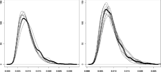
Figure 1: Estimated densities of the distribution of the statistic $\sqrt{T}\sup_{(v,\omega)\in[0,1]^{2}}|\hat{D}_{T}(v,\omega)|$ under the null hypothesis. The dotted line is the estimated exact density while the solid lines corresponds to the estimated densities of the bootstrap approximations. Left panel: $N=8$; right panel: $N=16$.

bootstrap approximations each. Based on these bootstrap replications, we estimate the density of the corresponding bootstrap approximations of the test statistic as well. The plots comparing these densities are given in Figure 1 where the dotted line corresponds to the estimated exact density while the dashed lines show the $10$ estimated densities of the bootstrap approximations.

4.3 Size and power of the test

In this section, we investigate the size and power of the test (26) and the analogue based on the pre-periodogram. We also compare these methods with three other tests for stationarity, which recently have been proposed in the literature. All reported results are based on $200$ bootstrap replications and $1000$ simulation runs under the null hypothesis while we use $500$ simulation runs under the alternative. To study the approximation of the nominal level, we simulate $\operatorname{AR}(1)$ processes

$$X_{t}=\phi X_{t-1}+Z_{t},\qquad t\in\mathbb{Z},$$ (28)

and $\operatorname{MA}(1)$ processes

$$X_{t}=Z_{t}+\theta Z_{t-1},\qquad t\in\mathbb{Z},$$ (29)

for different values of the parameters $\phi$ and $\theta$, where the $Z_{t}$ are independent and standard normal distributed random variables throughout the whole section. The corresponding results are depicted in Tables 1 and 2, respectively, and we observe a precise approximation of the nominal level in the $\operatorname{AR}(1)$ case for $\phi\in\{-0.5,0,0.5,0.9\}$ and in the $\operatorname{MA}(1)$ case

Table 1: Rejection probabilities of the test (26) under the null hypothesis. The data was generated according to model (28)

			$\phi=-0.9$		$\phi=-0.5$		$\phi=0$		$\phi=0.5$		$\phi=0.9$
$T$	$N$	$M$	$5\%$	$10\%$	$5\%$	$10\%$	$5\%$	$10\%$	$5\%$	$10\%$	$5\%$	$10\%$
$64$	$8$	$8$	$0.021$	$0.069$	$0.025$	$0.060$	$0.035$	$0.086$	$0.050$	$0.099$	$0.044$	$0.108$
$128$	$16$	$8$	$0.022$	$0.063$	$0.031$	$0.077$	$0.042$	$0.081$	$0.034$	$0.092$	$0.050$	$0.099$
$128$	$8$	$16$	$0.020$	$0.066$	$0.030$	$0.076$	$0.038$	$0.083$	$0.055$	$0.102$	$0.038$	$0.081$
$256$	$32$	$8$	$0.028$	$0.078$	$0.040$	$0.086$	$0.051$	$0.106$	$0.053$	$0.111$	$0.051$	$0.111$
$256$	$16$	$16$	$0.016$	$0.063$	$0.038$	$0.089$	$0.044$	$0.085$	$0.045$	$0.080$	$0.033$	$0.085$
$256$	$8$	$32$	$0.022$	$0.068$	$0.036$	$0.083$	$0.051$	$0.098$	$0.050$	$0.102$	$0.051$	$0.105$
$512$	$64$	$8$	$0.020$	$0.073$	$0.054$	$0.103$	$0.052$	$0.084$	$0.042$	$0.090$	$0.039$	$0.112$
$512$	$32$	$16$	$0.023$	$0.070$	$0.046$	$0.083$	$0.044$	$0.090$	$0.049$	$0.092$	$0.038$	$0.080$
$512$	$16$	$32$	$0.029$	$0.067$	$0.038$	$0.079$	$0.056$	$0.098$	$0.052$	$0.099$	$0.048$	$0.101$
$512$	$8$	$64$	$0.025$	$0.070$	$0.050$	$0.102$	$0.047$	$0.101$	$0.051$	$0.112$	$0.054$	$0.105$

for $\theta\in\{-0.9,-0.5,0.5,0.9\}$ even for very small samples sizes. Furthermore, if $T$ gets larger, the results are basically not affected by the choice of $N$ in these cases. For $\phi=-0.9$, the nominal level is underestimated for our choice of $T$, but at least if $T$ grows the approximation of the nominal level becomes more precise.

Table 2: Rejection probabilities of the test (26) under the null hypothesis. The data was generated according to model (29)

			$\theta=-0.9$		$\theta=-0.5$		$\theta=0.5$		$\theta=0.9$
$T$	$N$	$M$	$5\%$	$10\%$	$5\%$	$10\%$	$5\%$	$10\%$	$5\%$	$10\%$
$64$	$8$	$8$	$0.024$	$0.073$	$0.027$	$0.060$	$0.045$	$0.091$	$0.045$	$0.096$
$128$	$16$	$8$	$0.033$	$0.071$	$0.037$	$0.085$	$0.043$	$0.087$	$0.029$	$0.076$
$128$	$8$	$16$	$0.028$	$0.063$	$0.031$	$0.071$	$0.050$	$0.102$	$0.028$	$0.085$
$256$	$32$	$8$	$0.047$	$0.085$	$0.033$	$0.081$	$0.040$	$0.074$	$0.042$	$0.080$
$256$	$16$	$16$	$0.044$	$0.095$	$0.031$	$0.080$	$0.043$	$0.083$	$0.035$	$0.076$
$256$	$8$	$16$	$0.029$	$0.074$	$0.034$	$0.081$	$0.059$	$0.112$	$0.038$	$0.076$
$512$	$64$	$8$	$0.038$	$0.084$	$0.041$	$0.087$	$0.052$	$0.106$	$0.041$	$0.089$
$512$	$32$	$16$	$0.047$	$0.091$	$0.043$	$0.073$	$0.047$	$0.094$	$0.050$	$0.100$
$512$	$16$	$32$	$0.036$	$0.085$	$0.044$	$0.082$	$0.050$	$0.093$	$0.050$	$0.087$
$512$	$8$	$64$	$0.051$	$0.094$	$0.040$	$0.078$	$0.070$	$0.116$	$0.037$	$0.080$

To study the power of the test (26), we simulate data from the following four models which all correspond to the alternative of non-stationary processes. In particular, we consider

$$X_{t,T} = (1+t/T)Z_{t},$$ (30)

$$X_{t,T} = -0.9\sqrt{\frac{t}{T}}X_{t-1,T}+Z_{t},$$ (31)

$$X_{t,T} = \cases{0.5X_{t-1}+Z_{t},&\quad if $\displaystyle 1\leq t\leq\frac{T}{2}$,\cr-0.5X_{t-1}+Z_{t},&\quad if $\displaystyle\frac{T}{2}+1\leq t\leq T$,}$$ (32)

$$X_{t,T} = Z_{t}+0.8\cos\bigl{(}1.5-\cos(4\uppi t/T)\bigr{)}Z_{t-q},$$ (33)

where we display the results for the last model for different $q\in\mathbb{N}$. Note that due to Remark 2.5 the alternative (32) also fits into the theoretical framework. The corresponding rejection probabilities are reported in Table 3 and we observe a reasonable behavior of the procedure in the first three considered cases, whereas power is rather low for the alternative (33). Similar to the null hypothesis we observe robustness with respect to different choices of $N$, and even for the choice $M=32$, $N=8$, which appears to be implausible in view of (9), the results are satisfying. It might be of interest to compare these results both with the pre-periodogram approach from Theorem 2.2 and with other tests for the hypothesis of stationarity which have been recently suggested in the literature. In particular, we consider the tests of Paparoditis [23], Dwivedi and Subba Rao [15] and Dette, Preuss and Vetter [14].

Table 3: Rejection probabilities of the test (26) for several alternatives

			(30)		(31)		(32)		(33) $q=1$		(33) $q=6$
$T$	$N$	$M$	$5\%$	$10\%$	$5\%$	$10\%$	$5\%$	$10\%$	$5\%$	$10\%$	$5\%$	$10\%$
$64$	$8$	$8$	$0.286$	$0.444$	$0.186$	$0.328$	$0.168$	$0.270$	$0.046$	$0.098$	$0.052$	$0.104$
$128$	$16$	$8$	$0.686$	$0.772$	$0.396$	$0.546$	$0.308$	$0.466$	$0.090$	$0.154$	$0.072$	$0.130$
$128$	$8$	$16$	$0.624$	$0.758$	$0.382$	$0.578$	$0.410$	$0.548$	$0.082$	$0.144$	$0.080$	$0.136$
$256$	$32$	$8$	$0.958$	$0.974$	$0.672$	$0.814$	$0.742$	$0.912$	$0.110$	$0.186$	$0.102$	$0.166$
$256$	$16$	$16$	$0.942$	$0.978$	$0.698$	$0.814$	$0.640$	$0.806$	$0.118$	$0.202$	$0.098$	$0.166$
$256$	$8$	$32$	$0.944$	$0.970$	$0.760$	$0.868$	$0.672$	$0.808$	$0.118$	$0.210$	$0.086$	$0.144$

In Table 4, we present the rejection frequencies for the test based on the pre-periodogram as defined in (2). Recall that the use of the pre-periodogram does not require the specification of the value $N$, which specifies the number of observations for the calculation of the local periodogram. This makes its use attractive for practitioners. However, the results of the simulation study show that compared to the local periodogram the use of the pre-periodogram yields to a substantial loss of power for all four alternatives. In particular for alternatives of the form (32), the test cannot be recommended.

Table 4: Rejection probabilities of the test based on the pre-periodogram for several alternatives

	(30)		(31)		(32)		(33) $q=1$		(33) $q=6$
$T$	$5\%$	$10\%$	$5\%$	$10\%$	$5\%$	$10\%$	$5\%$	$10\%$	$5\%$	$10\%$
$64$	$0.188$	$0.340$	$0.080$	$0.202$	$0.022$	$0.056$	$0.024$	$0.076$	$0.044$	$0.102$
$128$	$0.552$	$0.702$	$0.216$	$0.392$	$0.036$	$0.116$	$0.038$	$0.086$	$0.052$	$0.098$
$256$	$0.938$	$0.968$	$0.580$	$0.734$	$0.080$	$0.176$	$0.062$	$0.150$	$0.088$	$0.132$

In Table 5, we show the corresponding rejection probabilities for the test proposed in Dette, Preuss and Vetter [14], which is the only of the remaining methods depending on one regularization parameter only. These authors proposed to estimate the $L_{2}$ distance

$$\int_{0}^{1}\int_{0}^{\uppi}\biggl{(}f(u,\lambda)-\int_{0}^{1}f(v,\lambda)\,\mathrm{d}v\biggr{)}^{2}\,\mathrm{d}\lambda\,\mathrm{d}u$$

using sums of the (squared) periodogram. In order to provide a fair comparison between the two methods, we also employ the $\operatorname{AR}(\infty)$ bootstrap to the corresponding test to generate critical values. It turns out that without a bootstrap the method of Dette, Preuss and Vetter [14] is much more sensitive with respect to different choices of $N$. We observe that the new method also outperforms the test proposed by Dette, Preuss and Vetter [14] in the alternatives (30) and (31). In most cases the differences are substantial. On the other hand, for the alternative (32) the procedure of Dette, Preuss and Vetter [14] has larger power if $T=64$ and $T=128$, but for $T=256$ the novel method performs better in this case as well. Nevertheless, the new approach is clearly outperformed by the proposal of Dette, Preuss and Vetter [14] for the alternative (33).

Table 5: Rejection probabilities of the test proposed by Dette, Preuss and Vetter [14] for several alternatives (quantiles obtained by $\operatorname{AR}(\infty)$ bootstrap)

			(30)		(31)		(32)		(33) $q=1$		(33) $q=6$
$T$	$N$	$M$	$5\%$	$10\%$	$5\%$	$10\%$	$5\%$	$10\%$	$5\%$	$10\%$	$5\%$	$10\%$
$64$	$8$	$8$	$0.116$	$0.196$	$0.188$	$0.232$	$0.250$	$0.344$	$0.244$	$0.350$	$0.056$	$0.116$
$128$	$16$	$8$	$0.106$	$0.160$	$0.256$	$0.330$	$0.370$	$0.552$	$0.490$	$0.584$	$0.226$	$0.336$
$128$	$8$	$16$	$0.168$	$0.268$	$0.220$	$0.286$	$0.432$	$0.566$	$0.398$	$0.516$	$0.072$	$0.126$
$256$	$32$	$8$	$0.378$	$0.498$	$0.282$	$0.412$	$0.746$	$0.922$	$0.740$	$0.836$	$0.532$	$0.670$
$256$	$16$	$16$	$0.208$	$0.368$	$0.276$	$0.410$	$0.618$	$0.794$	$0.716$	$0.816$	$0.342$	$0.444$
$256$	$8$	$32$	$0.224$	$0.338$	$0.300$	$0.418$	$0.582$	$0.744$	$0.620$	$0.760$	$0.104$	$0.178$

Table 6: Rejection probabilities of the test proposed by Paparoditis [23] for several alternatives (quantiles obtained by $\operatorname{AR}(\infty)$ bootstrap)

			(30)		(31)		(32)		(33) $q=1$		(33) $q=6$
$T$	$N$	$M$	$5\%$	$10\%$	$5\%$	$10\%$	$5\%$	$10\%$	$5\%$	$10\%$	$5\%$	$10\%$
$64$	$8$	$8$	$0.054$	$0.126$	$0.050$	$0.122$	$0.078$	$0.170$	$0.058$	$0.104$	$0.034$	$0.064$
$128$	$16$	$8$	$0.150$	$0.242$	$0.158$	$0.262$	$0.112$	$0.198$	$0.128$	$0.218$	$0.082$	$0.140$
$128$	$8$	$16$	$0.066$	$0.154$	$0.120$	$0.254$	$0.166$	$0.270$	$0.080$	$0.170$	$0.034$	$0.066$
$256$	$32$	$8$	$0.304$	$0.424$	$0.248$	$0.380$	$0.298$	$0.448$	$0.288$	$0.428$	$0.102$	$0.180$
$256$	$16$	$16$	$0.234$	$0.344$	$0.276$	$0.404$	$0.258$	$0.374$	$0.288$	$0.420$	$0.120$	$0.174$
$256$	$8$	$32$	$0.126$	$0.226$	$0.240$	$0.374$	$0.298$	$0.376$	$0.158$	$0.266$	$0.050$	$0.106$

In Table 6, we show the rejection frequencies for the method which was proposed in Paparoditis [23]. This concept basically works by estimating

$$\sup_{v\in[0,1]}\int_{-\uppi}^{\uppi}\biggl{(}\frac{f(v,\lambda)}{\int_{0}^{1}f(u,\lambda)\,\mathrm{d}u}-1\biggr{)}^{2}\,\mathrm{d}\lambda$$

via a smoothed local periodogram, which requires the choice of a smoothing bandwidth besides the window length $N$. We choose the uniform kernel function, and as recommended by the author we select the bandwidth via the cross validation criterion of Beltrão and Bloomfield [2]. To provide a fair comparison, we also use the $\operatorname{AR}(\infty)$ bootstrap to obtain critical values. For the alternatives (30)–(32) the proposal of Paparoditis [23] yields substantial less power than the approach proposed in this paper, whereas for the alternative (33) no clear picture can be drawn. For $q=1$, the method of Paparoditis [23] performs better, while there is no significant difference in the performance if $q=6$. In any case, Paparoditis [23] is clearly outperformed by the approach of Dette, Preuss and Vetter [14] for (33).

Finally, we compare our approach to that proposed in Dwivedi and Subba Rao [15]. These authors suggested a Portmanteau type test by estimating

$$T\sum_{r=1}^{m}\bigl{|}c_{T}(r)\bigr{|}^{2},$$

where $c_{T}(r)$ is the covariance of the process at lag $r$. For the estimation of $c_{T}(r)$, the authors require the choice of a smoothing bandwidth, and again we use the cross validation criterion and the uniform kernel function. Dwivedi and Subba Rao [15] also have to choose the maximal lag $m\in N$ up to which they want to estimate $c_{T}(r)$, and we pick $m=5$ in the simulations. As in the other examples, we employ the $\operatorname{AR}(\infty)$ bootstrap, and the results are given in Table 7. A comparison with our method yields a

Table 7: Rejection probabilities of the test proposed by Dwivedi and Subba Rao [15] for several alternatives (quantiles obtained by $\operatorname{AR}(\infty)$ bootstrap)

	(30)		(31)		(32)		(33) $q=1$		(33) $q=6$
$T$	$5\%$	$10\%$	$5\%$	$10\%$	$5\%$	$10\%$	$5\%$	$10\%$	$5\%$	$10\%$
$64$	$0.174$	$0.266$	$0.056$	$0.100$	$0.082$	$0.164$	$0.072$	$0.120$	$0.046$	$0.098$
$128$	$0.274$	$0.386$	$0.058$	$0.114$	$0.122$	$0.208$	$0.126$	$0.206$	$0.092$	$0.162$
$256$	$0.604$	$0.716$	$0.128$	$0.210$	$0.174$	$0.276$	$0.234$	$0.340$	$0.174$	$0.272$

result similar to the approach of Paparoditis [23]. Our approach performs better for the alternatives (30)–(32) while the proposal of Dwivedi and Subba Rao [15] yields a higher power in model (33). Again it is clearly outperformed in this case by the test proposed in Dette, Preuss and Vetter [14].

4.4 Data example

As an illustration, we consider $T=257$ observations of weekly egg prices at a German agriculture market between April 1967 and March 1972. A plot of the data is given in Figure 2, and following Paparoditis [23] the first order difference $\Delta_{t}=X_{t}-X_{t-1}$ of the observed time series are analyzed. Although several stationary models were proposed in the literature to fit this data (cf. Paparoditis [23]), the new test rejects the null hypothesis with $p$-value $0.006$ if we choose $N=32$ or $N=16$, and with $p$-value $0.001$ if we choose $N=8$. These results demonstrate again that the choice of $N$ does not have too much influence on the outcome, and that even the somewhat implausible choice of $N=8$ yields a $p$-value similar to the others.

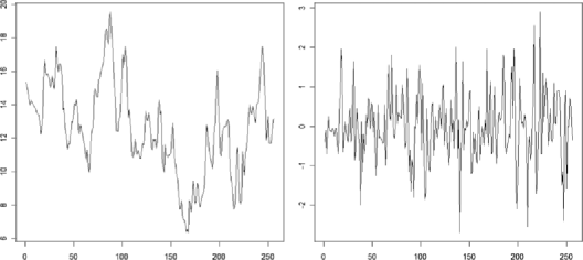
Figure 2: Left panel: Weekly egg prices at a German agriculture market between April 1967 and March 1972. Right panel: First order difference of the weekly egg prices.

Note that in Paparoditis [23] a longer version of the above time series was analyzed, namely $1201$ observations of weekly egg prices between April 1967 and May 1990. However, we obtain a $p$-value of exactly $0$ even if we choose $10^{6}$ bootstrap replicates in this case, which is why we consider the first $257$ datapoints only. Paparoditis [23] rejects the null hypothesis of stationarity at level $5\%$ if the whole dataset is used, but his approach yields a $p$-value of $0.1834$ if it is applied to the first $257$ observations of the time series only, and therefore the hypothesis of stationarity cannot be rejected at a reasonable size using his method. Roughly the same $p$-value, namely $0.189$, can be observed if the approach of Dwivedi and Subba Rao [15] is employed.

Appendix: Proofs

.1 Proof of Theorem 2.1

Throughout the proof, we set $y_{j}=(v_{j},\omega_{j})\in[0,1]^{2}$ for $j=1,\ldots,K$ and $K\in\mathbb{N}$. To show weak convergence we follow Theorems 1.5.4 and 1.5.7 in van der Vaart and Wellner [28] and prove the following two claims:

1. [(2)]

2. Convergence of the finite dimensional distributions, that is,

   $$\bigl{(}\hat{G}_{T}(y_{j})\bigr{)}_{j=1,\ldots,K}\stackrel{{\scriptstyle D}}{{\longrightarrow}}\bigl{(}G(y_{j})\bigr{)}_{j=1,\ldots,K}.$$ (1)

3. Stochastic equicontinuity, that is,

   $$\forall\eta,\varepsilon>0\ \exists\delta>0\colon\ \qquad\lim_{T\rightarrow\infty}P\Bigl{(}\sup_{y_{1},y_{2}\in[0,1]^{2}\mathchoice{\nobreak\,\colon}{\nobreak\,\colon}{\nobreak\,\colon\;}{\nobreak\,\colon\;}d_{2}(y_{1},y_{2})<\delta}\bigl{|}G_{T}(y_{1})-G_{T}(y_{2})\bigr{|}>\eta\Bigr{)}<\varepsilon,$$ (2)

   where $d_{2}(y_{1},y_{2})=\sqrt{(v_{1}-v_{2})^{2}+(w_{1}-w_{2})^{2}}$.

Proof of (1) The claim follows from similar arguments as given in the proof of Theorem 3.1 in Dette, Preuss and Vetter [14]. For the sake of brevity and because we will use similar arguments in the proof of (2), we will sketch how the assertions

$$\mathbb{E}\bigl{(}\hat{G}_{T}(v,\omega)\bigr{)} \stackrel{{\scriptstyle T\rightarrow\infty}}{{\hbox to28.45274pt{\rightarrowfill}}} 0,$$ (3)

$$\operatorname{Cov}\bigl{(}\hat{G}_{T}(y_{1}),\hat{G}_{T}(y_{2})\bigr{)} \stackrel{{\scriptstyle T\rightarrow\infty}}{{\hbox to28.45274pt{\rightarrowfill}}} \frac{1}{2\uppi}\int_{0}^{1}\int_{0}^{\uppi\min(\omega_{1},\omega_{2})}\bigl{(}1_{[0,v_{1}]}(u)-v_{1}\bigr{)}\bigl{(}1_{[0,v_{2}]}(u)-v_{2}\bigr{)}$$

$$\hskip 83.4pt{}\times f^{2}(u,\lambda)\,\mathrm{d}\lambda\,\mathrm{d}u$$

can be shown. Note that we have

$$\hat{G}_{T}(v,\omega) = \frac{1}{\sqrt{T}}\sum_{j=1}^{M}\sum_{k=1}^{{N}/{2}}\phi_{v,\omega,M,N}(u_{j},\lambda_{k})I_{N}^{X}(u_{j},\lambda_{k})-\sqrt{T}D_{N,M}(\phi_{v,\omega,M,N})$$

$$= \!:G_{T}(\phi_{v,\omega,M,N})$$

with

$$\phi_{v,\omega,M,N}(u,\lambda):=\biggl{(}I_{[0,{\lfloor vM\rfloor}/{M}]}(u)-\frac{\lfloor vM\rfloor}{M}\biggr{)}I_{[0,{2\uppi\lfloor\omega{N}/{2}\rfloor/N}]}(\lambda)$$

for $u,\lambda\geq 0$ and

$$D_{N,M}(\phi):=\frac{1}{2\uppi}\int_{0}^{1}\int_{0}^{\uppi}\phi(u,\lambda)f(u,\lambda)\,\mathrm{d}\lambda\,\mathrm{d}u.$$

In order to simplify some technical arguments, we also define

$$\phi_{v,\omega,M,N}(u,\lambda):=\phi_{v,\omega,M,N}(u,-\lambda)$$

for $u\geq 0,\lambda<0$ and obtain from (3)

$$\mathbb{E}\Biggl{(}\frac{1}{T}\sum_{j=1}^{M}\sum_{k=1}^{{N}/{2}}\phi_{v,\omega,M,N}(u_{j},\lambda_{k})I_{N}^{X}(u_{j},\lambda_{k})\Biggr{)}$$

$$\quad=\frac{1}{T}\sum_{j=1}^{M}\sum_{k=1}^{{N}/{2}}\phi_{v,\omega,M,N}(u_{j},\lambda_{k})$$

$$\hskip 39.6pt\qquad{}\times\frac{1}{2\uppi N}\sum_{p,q=0}^{N-1}\sum_{l,m=-\infty}^{\infty}\psi_{l}\biggl{(}\frac{t_{j}-N/2+1+p}{T}\biggr{)}\psi_{m}\biggl{(}\frac{t_{j}-N/2+1+q}{T}\biggr{)}$$

$$\hskip 151.3pt{}\times\mathbb{E}(Z_{t_{j}-N/2+1+p-m}Z_{t_{j}-N/2+1+q-l})$$

$$\hskip 151.3pt{}\times\exp\bigl{(}-\mathrm{i}\lambda_{k}(p-q)\bigr{)}\bigl{(}1+\mathrm{O}(1/T)\bigr{)}.$$

A Taylor expansion now yields that this term becomes

$$\frac{1}{T}\sum_{j=1}^{M}\sum_{k=1}^{{N}/{2}}\phi_{v,\omega,M,N}(u_{j},\lambda_{k})\frac{1}{2\uppi N}$$

$$\hskip 39.0pt{}\times\sum_{p,q=0}^{N-1}\sum_{l,m=-\infty}^{\infty}\psi_{l}(u_{j})\psi_{m}(u_{j})$$

$$\hskip 103.0pt{}\times\mathbb{E}(Z_{t_{j}-N/2+1+p-m}Z_{t_{j}-N/2+1+q-l})$$

$$\hskip 103.0pt{}\times\exp\bigl{(}-\mathrm{i}\lambda_{k}(p-q)\bigr{)}\bigl{(}1+\mathrm{O}(1/T)+\mathrm{O}\bigl{(}N^{2}/T^{2}\bigr{)}\bigr{)}.$$

See Dette, Preuss and Vetter [14] for details. Since $\mathbb{E}(Z_{i}Z_{j})=0$ for $i\not=j$, we obtain the equation $p=q+m-l$ which shows that the above expression equals

$$\frac{1}{2\uppi NT}\sum_{j=1}^{M}\sum_{k=1}^{{N}/{2}}\phi_{v,\omega,M,N}(u_{j},\lambda_{k})$$

$$\qquad\hskip 39.0pt{}\times\sum_{l,m=-\infty}^{\infty}\mathop{\sum_{q=0}}_{0\leq q+m-l\leq N-1}^{N-1}\psi_{l}(u_{j})\psi_{m}(u_{j})\exp\bigl{(}-\mathrm{i}\lambda_{k}(m-l)\bigr{)}$$

$$\qquad{}+\mathrm{O}(1/T)+\mathrm{O}\bigl{(}N^{2}/T^{2}\bigr{)}$$

$$\quad=\frac{1}{2\uppi NT}\sum_{j=1}^{M}\sum_{k=1}^{{N}/{2}}\phi_{v,\omega,M,N}(u_{j},\lambda_{k})$$

$$\qquad\hskip 59.3pt{}\times\mathop{\sum_{l,m=-\infty}}_{|l-m|\leq N-1}^{\infty}\mathop{\sum_{q=0}}_{0\leq q+m-l\leq N-1}^{N-1}\psi_{l}(u_{j})\psi_{m}(u_{j})\exp\bigl{(}-\mathrm{i}\lambda_{k}(m-l)\bigr{)}$$

$$\qquad{}+\frac{1}{2\uppi NT}\sum_{j=1}^{M}\sum_{k=1}^{{N}/{2}}\phi_{v,\omega,M,N}(u_{j},\lambda_{k})$$

$$\qquad\hskip 71.5pt{}\times\mathop{\sum_{l,m=-\infty}}_{|l-m|\geq N}^{\infty}\mathop{\sum_{q=0}}_{0\leq q+m-l\leq N-1}^{N-1}\psi_{l}(u_{j})\psi_{m}(u_{j})\exp\bigl{(}-\mathrm{i}\lambda_{k}(m-l)\bigr{)}$$

$$\qquad{}+\mathrm{O}(1/T)+\mathrm{O}\bigl{(}N^{2}/T^{2}\bigr{)}.$$

Dropping the extra condition $0\leq q+m-l\leq N-1$, the second term is bounded by

$$C\mathop{\sum_{l,m=-\infty}}_{|l-m|\geq N}^{\infty}\sup_{u}\bigl{|}\psi_{l}(u)\bigr{|}\sup_{u}\bigl{|}\psi_{m}(u)\bigr{|} \leq 2C\sum_{m=-\infty}^{\infty}\sup_{u}\bigl{|}\psi_{m}(u)\bigr{|}\mathop{\sum_{l=-\infty}}_{|l|\geq N/2}^{\infty}\sup_{u}\bigl{|}\psi_{l}(u)\bigr{|}$$

$$\leq \frac{4C\sum_{m=-\infty}^{\infty}\sup_{u}|\psi_{m}(u)|\sum_{l=-\infty}^{\infty}|l|\sup_{u}|\psi_{l}(u)|}{N}\hskip 29.0pt$$

$$= \mathrm{O}(1/N)$$

for some $C\in\mathbb{R}$ and the order follows from (4). Using (4) and (.1) in the same way again, the first quantity above can be shown to be equal to

$$\frac{1}{2\uppi T}\sum_{j=1}^{M}\sum_{k=1}^{{N}/{2}}\phi_{v,\omega,M,N}(u_{j},\lambda_{k})\sum_{l,m=-\infty}^{\infty}\psi_{l}(u_{j})\psi_{m}(u_{j})\exp\bigl{(}-\mathrm{i}\lambda_{k}(m-l)\bigr{)}+\mathrm{O}(1/N),$$

and therefore we obtain

$$\mathbb{E}\Biggl{(}\frac{1}{T}\sum_{j=1}^{M}\sum_{k=1}^{{N}/{2}}\phi_{v,\omega,M,N}(u_{j},\lambda_{k})I_{N}^{X}(u_{j},\lambda_{k})\Biggr{)}$$

$$\quad=\frac{1}{T}\sum_{j=1}^{M}\sum_{k=1}^{{N}/{2}}\phi_{v,\omega,M,N}(u_{j},\lambda_{k})f(u_{j},\lambda_{k})+\mathrm{O}(1/N)$$

$$\qquad{}+\mathrm{O}\bigl{(}N^{2}/T^{2}\bigr{)}+\mathrm{O}(1/T)$$

$$\quad=D_{N,M}(\phi_{v,\omega,M,N})+\mathrm{O}(1/N)+\mathrm{O}\bigl{(}N^{2}/T^{2}\bigr{)}+\mathrm{O}(1/T),$$

where the order of the Riemann approximation follows from the specific choice of the midpoints $u_{j}$. This together with (9) yields (3).

To prove (.1), we use symmetry arguments and obtain

$$T\operatorname{cum}\Biggl{(}\frac{1}{T}\sum_{j_{1}=1}^{M}\sum_{k_{1}=1}^{{N}/{2}}\phi_{v_{1},\omega_{1},M,N}(u_{j_{1}},\lambda_{k_{1}})I_{N}^{X}(u_{j_{1}},\lambda_{k_{1}}),$$

$$\hskip 33.3pt\frac{1}{T}\sum_{j_{2}=1}^{M}\sum_{k_{2}=1}^{{N}/{2}}\phi_{v_{2},\omega_{2},M,N}(u_{j_{2}},\lambda_{k_{2}})I_{N}^{X}(u_{j_{2}},\lambda_{k_{2}})\Biggr{)}$$

$$\quad=\frac{1}{4T}\frac{1}{(2\uppi N)^{2}}\sum_{j_{1},j_{2}=1}^{M}\sum_{k_{1},k_{2}=-\lfloor({N-1})/{2}\rfloor}^{{N}/{2}}\phi_{v_{1},\omega_{1},M,N}(u_{j_{1}},\lambda_{k_{1}})\phi_{v_{2},\omega_{2},M,N}(u_{j_{2}},\lambda_{k_{2}})$$

$$\qquad{}\times\sum_{p_{1},p_{2},q_{1},q_{2}=0}^{N-1}\sum_{m_{1},m_{2},l_{1},l_{2}=-\infty}^{\infty}\psi_{m_{1}}(u_{j_{1}})\psi_{l_{1}}(u_{j_{1}})\psi_{m_{2}}(u_{j_{2}})\psi_{l_{2}}(u_{j_{2}})$$

$$\hskip 116.5pt\qquad{}\times\exp\bigl{(}-\mathrm{i}\lambda_{k_{1}}(p_{1}-q_{1})\bigr{)}\exp\bigl{(}-\mathrm{i}\lambda_{k_{2}}(p_{2}-q_{2})\bigr{)}$$

$$\hskip 116.5pt\qquad{}\times\operatorname{cum}(Z_{t_{j_{1}}-N/2+1+p_{1}-m_{1}}Z_{t_{j_{1}}-N/2+1+q_{1}-l_{1}},$$

$$\hskip 149.7pt\qquad{}Z_{t_{j_{2}}-N/2+1+p_{2}-m_{2}}Z_{t_{j_{2}}-N/2+1+q_{2}-l_{2}})$$

$$\hskip 116.5pt\qquad{}\times\bigl{(}1+\mathrm{O}\bigl{(}N^{2}/T^{2}\bigr{)}+\mathrm{O}(1/T)\bigr{)}$$

in the same way as above. Because of

$$\operatorname{cum}(Z_{t_{j_{1}}-N/2+1+p_{1}-m_{1}}Z_{t_{j_{1}}-N/2+1+q_{1}-l_{1}},Z_{t_{j_{2}}-N/2+1+p_{2}-m_{2}}Z_{t_{j_{2}}-N/2+1+q_{2}-l_{2}})$$

$$\!\!\quad=\operatorname{cum}(Z_{t_{j_{1}}-N/2+1+p_{1}-m_{1}}Z_{t_{j_{2}}-N/2+1+q_{2}-l_{2}})\operatorname{cum}(Z_{t_{j_{2}}-N/2+1+p_{2}-m_{2}}Z_{t_{j_{1}}-N/2+1+q_{1}-l_{1}})$$

$$\!\!\qquad{}+\operatorname{cum}(Z_{t_{j_{1}}-N/2+1+p_{1}-m_{1}}Z_{t_{j_{2}}-N/2+1+p_{2}-m_{2}})\operatorname{cum}(Z_{t_{j_{1}}-N/2+1+q_{1}-l_{1}}Z_{t_{j_{2}}-N/2+1+q_{2}-l_{2}}),$$

the calculation of the highest order term in the variance splits into two sums and we only consider the first one (the second sum is treated completely analogously), which equals

$$\frac{1}{4T}\sum_{j_{1},j_{2}=1}^{M}\sum_{k_{1},k_{2}=-\lfloor({N-1})/{2}\rfloor}^{{N}/{2}}\phi_{v_{1},\omega_{1},M,N}(u_{j_{1}},\lambda_{k_{1}})\phi_{v_{2},\omega_{2},M,N}(u_{j_{2}},\lambda_{k_{2}})\frac{1}{(2\uppi N)^{2}}$$

$$\qquad{}\times\sum_{m_{1},m_{2},l_{1},l_{2}=-\infty}^{\infty}\mathop{\mathop{\sum_{q_{1},q_{2}=0}}_{0\leq q_{2}+m_{1}-l_{2}+t_{j_{2}}-t_{j_{1}}\leq N-1}}_{0\leq q_{1}+m_{2}-l_{1}+t_{j_{1}}-t_{j_{2}}\leq N-1}^{N-1}\psi_{m_{1}}(u_{j_{1}})\psi_{l_{1}}(u_{j_{1}})\psi_{m_{2}}(u_{j_{2}})\psi_{l_{2}}(u_{j_{2}})$$

$$\hskip 184.0pt{}\times\exp\bigl{(}-\mathrm{i}(\lambda_{k_{1}}-\lambda_{k_{2}})(q_{2}-q_{1}+t_{j_{2}}-t_{j_{1}})\bigr{)}$$

$$\hskip 184.0pt{}\times\exp\bigl{(}-\mathrm{i}\lambda_{k_{1}}(m_{1}-l_{2})-\mathrm{i}\lambda_{k_{2}}(m_{2}-l_{1})\bigr{)}$$

$$\quad=\frac{1}{4T}\sum_{j_{1},j_{2}=1}^{M}\sum_{k_{1},k_{2}=-\lfloor({N-1})/{2}\rfloor}^{{N}/{2}}\phi_{v_{1},\omega_{1},M,N}(u_{j_{1}},\lambda_{k_{1}})\phi_{v_{2},\omega_{2},M,N}(u_{j_{2}},\lambda_{k_{2}})\frac{1}{(2\uppi N)^{2}}$$

$$\qquad{}\times\mathop{\sum_{m_{1},m_{2},l_{1},l_{2}=-\infty}}_{(+)}^{\infty}\mathop{\mathop{\sum_{q_{1},q_{2}=0}}_{0\leq q_{2}+m_{1}-l_{2}+t_{j_{2}}-t_{j_{1}}\leq N-1}}_{0\leq q_{1}+m_{2}-l_{1}+t_{j_{1}}-t_{j_{2}}\leq N-1}^{N-1}\psi_{m_{1}}(u_{j_{1}})\psi_{l_{1}}(u_{j_{1}})\psi_{m_{2}}(u_{j_{2}})\psi_{l_{2}}(u_{j_{2}})$$

$$\hskip 184.0pt{}\times\exp\bigl{(}-\mathrm{i}(\lambda_{k_{1}}-\lambda_{k_{2}})(q_{2}-q_{1}+t_{j_{2}}-t_{j_{1}})\bigr{)}$$

$$\hskip 184.0pt{}\times\exp\bigl{(}-\mathrm{i}\lambda_{k_{1}}(m_{1}-l_{2})-\mathrm{i}\lambda_{k_{2}}(m_{2}-l_{1})\bigr{)}$$

$$\hskip 184.0pt{}\times\bigl{(}1+\mathrm{O}(1/N)\bigr{)},$$

where $\sum_{(+)}$ means that summation is only performed over those indices $x,y\in\{m_{1},m_{2},l_{1},l_{2}\}$ such that $|x-y|<N$, and the $\mathrm{O}(1/N)$-term follows with (.1). Assume that $j_{1}$ has been chosen. Then $j_{2}$ must be equal to $j_{1},j_{1}-1$ or $j_{1}+1$, as all other combination of $j_{1}$ and $j_{2}$ vanish, because of the condition $0\leq q_{2}+m_{1}-l_{2}+t_{j_{2}}-t_{j_{1}}\leq N-1$ and the fact that the summation is only performed with respect to the indices satisfying $|x-y|<N$. If $j_{2}$ equals $j_{1}-1$ or $j_{1}+1$, it follows from the conditions on $q_{1}$ and $q_{2}$ that for chosen $m_{i}$ and $l_{i}$, there are at most $|m_{2}-l_{1}|$ possible choices for $q_{1}$ and at most $|m_{1}-l_{2}|$ possible choices for $q_{2}$. It therefore follows with (4) that the terms with $j_{2}\in\{j_{1}-1,j_{1}+1\}$ are of order $\mathrm{O}(1/N)$.

Therefore, we only have to consider the case $j_{1}=j_{2}$, and the above expression is

$$\frac{1}{4T}\sum_{j_{1}=1}^{M}\sum_{k_{1},k_{2}=-\lfloor({N-1})/{2}\rfloor}^{{N}/{2}}\phi_{v_{1},\omega_{1},M,N}(u_{j_{1}},\lambda_{k_{1}})\phi_{v_{2},\omega_{2},M,N}(u_{j_{1}},\lambda_{k_{2}})$$

$$\quad{}\times\frac{1}{(2\uppi N)^{2}}\mathop{\sum_{m_{1},m_{2},l_{1},l_{2}=-\infty}}_{(+)}^{\infty}\mathop{\mathop{\sum_{q_{1},q_{2}=0}}_{0\leq q_{2}+m_{1}-l_{2}\leq N-1}}_{0\leq q_{1}+m_{2}-l_{1}\leq N-1}^{N-1}\psi_{m_{1}}(u_{j_{1}})\psi_{l_{1}}(u_{j_{1}})\psi_{m_{2}}(u_{j_{2}})\psi_{l_{2}}(u_{j_{2}})$$

$$\hskip 171.0pt\quad{}\times\exp\bigl{(}-\mathrm{i}(\lambda_{k_{1}}-\lambda_{k_{2}})(q_{2}-q_{1})\bigr{)}$$ (6)

$$\hskip 171.0pt\quad{}\times\exp\bigl{(}-\mathrm{i}\lambda_{k_{1}}(m_{1}-l_{2})-\mathrm{i}\lambda_{k_{2}}(m_{2}-l_{1})\bigr{)}\hskip 27.0pt$$

$$\hskip 171.0pt\quad{}\times\bigl{(}1+\mathrm{O}(1/N)\bigr{)}.$$

Observing

$$\frac{1}{N}\sum_{q=0}^{N-1}\exp\bigl{(}-\mathrm{i}(\lambda_{k_{1}}-\lambda_{k_{2}})q\bigr{)}=\cases{1,&\quad$k_{1}-k_{2}=lN$ with $l\in\mathbb{Z}$,\cr 0,&\quad else,}$$

it follows that for fixed $m_{1}$, $l_{2}$ and $k_{1}\not=k_{2}$ we have

$$\Biggl{|}\mathop{\sum_{q_{2}=0}}_{0\leq q_{2}+m_{1}-l_{2}\leq N-1}^{N-1}\exp\bigl{(}-\mathrm{i}(\lambda_{k_{1}}-\lambda_{k_{2}})q_{2}\bigr{)}\Biggr{|} = \Biggl{|}\mathop{\mathop{\mathop{\sum_{q_{2}=0}}_{q_{2}+m_{1}-l_{2}<0}}_{\mathrm{or}}}_{q_{2}+m_{1}-l_{2}>N-1}^{N-1}\exp\bigl{(}-\mathrm{i}(\lambda_{k_{1}}-\lambda_{k_{2}})q_{2}\bigr{)}\Biggr{|}$$

$$\leq |m_{1}-l_{2}|,$$

which implies

$$\Biggl{|}\frac{1}{(2\uppi N)^{2}}\mathop{\mathop{\sum_{q_{1},q_{2}=0}}_{0\leq q_{2}+m_{1}-l_{2}\leq N-1}}_{0\leq q_{1}+m_{2}-l_{1}\leq N-1}^{N-1}\exp\bigl{(}-\mathrm{i}(\lambda_{k_{1}}-\lambda_{k_{2}})(q_{2}-q_{1})\bigr{)}\Biggr{|}\leq|m_{1}-l_{2}||m_{2}-l_{1}|/(2\uppi N)^{2}.$$ (7)

By using (4) and (7), it can now be seen that all terms with $k_{1}\not=k_{2}$ are of the order $\mathrm{O}(1/N)$, and similar arguments as used in the calculation of the expectation yield that (.1) equals

$$\frac{1}{4\uppi}\int_{0}^{1}\int_{0}^{\uppi\min(\omega_{1},\omega_{2})}\bigl{(}1_{[0,v_{1}]}(u)-v_{1}\bigr{)}\bigl{(}1_{[0,v_{2}]}(u)-v_{2}\bigr{)}f^{2}(u,\lambda)\,\mathrm{d}\lambda\,\mathrm{d}u$$

$$\quad{}+\mathrm{O}(1/N)+\mathrm{O}\bigl{(}N^{2}/T^{2}\bigr{)}.$$

Proof of (2) Note that

$$\mathcal{F}_{T}:=\bigl{\{}\phi_{v,\omega,M,N};v,\omega\in[0,1]\bigr{\}}=\bigl{\{}\phi_{v,\omega,M,N};(v,\omega)\in P_{T}\bigr{\}},$$

where

$$P_{T}:=\biggl{\{}0,\frac{1}{M},\frac{2}{M},\ldots,\frac{M-1}{M},1\biggr{\}}\times\biggl{\{}0,\frac{2}{N},\frac{4}{N},\ldots,1-\frac{2}{N},1\biggr{\}}$$

(recall that $N$ is assumed to be even throughout this paper). We define

$$\rho_{2}(\phi):=\biggl{(}\int_{0}^{1}\int_{0}^{\uppi}\phi^{2}(u,\lambda)\,\mathrm{d}\lambda\,\mathrm{d}u\biggr{)}^{1/2},$$

and $\mathcal{F}^{2}_{T}$ is the set of functions, which can be expressed as a sum or a difference of two elements in $\mathcal{F}_{T}$. The main task is to prove the following theorem.

Theorem .1

There exists a constant $C\in\mathbb{R}$ such that for all $\phi\in\mathcal{F}^{2}_{T}$:

$$\mathbb{E}\bigl{(}\bigl{|}\hat{G}_{T}(\phi)\bigr{|}^{k}\bigr{)}\leq(2k)!C^{k}\rho_{2}(\phi)^{k}\qquad\forall k\in\mathbb{N}\mbox{ even}.$$

Stochastic equicontinuity follows then by similar arguments as given in Dahlhaus [6], which is why we will only sketch the main steps and refer to his work for most details. The first consequence of Theorem .1 regards the existence of a constant $C_{1}\in\mathbb{R}$ such that for all $g,h\in\mathcal{F}_{T}$ and $\eta>0$:

$$P\bigl{(}\bigl{|}\hat{G}_{T}(g)-\hat{G}_{T}(h)\bigr{|}>\eta\rho_{2}(g-h)\bigr{)}\leq 96\exp\biggl{(}-\sqrt{\frac{\eta}{C_{1}}}\biggr{)}.$$

A straightforward modification of the chaining lemma in Chapter VII.2 of Pollard [24] then yields that for a stochastic process $(Z(v))_{v\in V}$, whose index set $V$ has a finite covering integral

$$J(\delta)=\int_{0}^{\delta}\biggl{[}\log\biggl{(}\frac{48N(u)^{2}}{u}\biggr{)}\biggr{]}^{2}\,\mathrm{d}u$$ (8)

for all $\delta$ and which satisfies

$$P\bigl{(}\bigl{|}Z(v)-Z(w)\bigr{|}>\nu d(v,w)\bigr{)}\leq 96\exp\biggl{(}-\sqrt{\frac{\nu}{C_{1}}}\biggr{)}$$

for a semi-metric $d$ on $V$ and a constant $C_{1}\in\mathbb{R}$, there exist a dense subset $V^{*}\subset V$ such that

$$P\bigl{(}\exists v,w\in V^{*}\mbox{ with }d(v,w)<\varepsilon\mbox{ and }\bigl{|}Z(v)-Z(w)\bigr{|}>26C_{1}J\bigl{(}d(v,w)\bigr{)}\bigr{)}\leq 2\varepsilon.$$

In (8), $N(u)$ is the covering number which is defined as the smallest number $m\in\mathbb{N}$ for which there exist $z_{1},\ldots,z_{m}\in V$ with $\min_{i}d(z,z_{i})\leq u$ for all $z\in V$. By using $y_{i}=(v_{i},\omega_{i})$, we obtain

$$P\Bigl{(}\sup_{y_{1},y_{2}\in P_{T}\mathchoice{\nobreak\,\colon}{\nobreak\,\colon}{\nobreak\,\colon\;}{\nobreak\,\colon\;}d_{2}(y_{1},y_{2})<\delta}\bigl{|}\hat{G}_{T}(v_{2},w_{2})-\hat{G}_{T}(v_{1},w_{1})\bigr{|}>\eta\Bigr{)}$$

$$\quad\leq P\Bigl{(}\sup_{f,g\in\mathcal{F}_{T}\mathchoice{\nobreak\,\colon}{\nobreak\,\colon}{\nobreak\,\colon\;}{\nobreak\,\colon\;}\rho_{2}(f,g)<\varepsilon(\delta)}\bigl{|}\hat{G}_{T}(f)-\hat{G}_{T}(g)\bigr{|}>\eta\Bigr{)}$$

for a certain sequence $\varepsilon(\delta)\stackrel{{\scriptstyle\delta\rightarrow 0}}{{\hbox to28.45274pt{\rightarrowfill}}}0$ by continuity. The right-hand side of this inequality equals

$$P\Bigl{(}\sup_{f,g\in\mathcal{F}_{T}\mathchoice{\nobreak\,\colon}{\nobreak\,\colon}{\nobreak\,\colon\;}{\nobreak\,\colon\;}\rho_{2}(f,g)<\varepsilon(\delta)}\bigl{|}\hat{G}_{T}(f)-\hat{G}_{T}(g)\bigr{|}>\eta,\eta\geq 26C_{1}J_{T}\bigl{(}\varepsilon(\delta)\bigr{)}\Bigr{)}$$

$$\qquad{}+P\Bigl{(}\sup_{f,g\in\mathcal{F}_{T}\mathchoice{\nobreak\,\colon}{\nobreak\,\colon}{\nobreak\,\colon\;}{\nobreak\,\colon\;}\rho_{2}(f,g)<\varepsilon(\delta)}\bigl{|}\hat{G}_{T}(f)-\hat{G}_{T}(g)\bigr{|}>\eta,\eta<26C_{1}J_{T}\bigl{(}\varepsilon(\delta)\bigr{)}\Bigr{)}$$

$$\quad\leq 2\varepsilon(\delta)+P\bigl{(}\eta<26C_{1}J_{T}\bigl{(}\varepsilon(\delta)\bigr{)}\bigr{)},$$

where $J_{T}(\delta)$ is the corresponding covering integral of $\mathcal{F}_{T}$. Note that $\eta<26C_{1}J_{T}(\varepsilon(\delta))$ is not random and that $J_{T}(\delta)$ can be bounded by $J(\delta)$, which is the covering integral of $\bigcup_{i=1}^{\infty}\mathcal{F}_{i}$ (which is finite for every $\delta$). Because of $J(\varepsilon(\delta))\stackrel{{\scriptstyle\delta\rightarrow 0}}{{\hbox to28.45274pt{\rightarrowfill}}}0$, we have $\eta>26C_{1}J(\delta)$ whenever $\delta$ is sufficiently small and obtain

$$P\Bigl{(}\sup_{f,g\in\mathcal{F}_{T}\mathchoice{\nobreak\,\colon}{\nobreak\,\colon}{\nobreak\,\colon\;}{\nobreak\,\colon\;}\rho_{2}(f,g)<\varepsilon(\delta)}\bigl{|}\hat{G}_{T}(f)-\hat{G}_{T}(g)\bigr{|}>\eta\Bigr{)}<2\varepsilon(\delta),$$

which implies the stochastic equicontinuity. Proof of Theorem .1 We show

$$\bigl{|}\operatorname{cum}_{l}\bigl{(}\sqrt{T}\hat{D}_{T}(\phi)\bigr{)}\bigr{|}\leq(2l)!\tilde{C}^{l}\rho_{2}(\phi)^{l}\qquad\forall l\in\mathbb{N},$$ (9)

where

$$\hat{D}_{T}(\phi):=\frac{1}{\sqrt{T}}\hat{G}_{T}(\phi)+D_{N,M}(\phi).$$

Since $D_{N,M}(\phi)$ is constant, this implies

$$\bigl{|}\operatorname{cum}_{l}(\hat{G}_{T})\bigr{|}\leq(2l)!C^{l}\rho_{2}(\phi)^{l}\qquad\forall l\in\mathbb{N}$$

for some $C$, and then it follows as in Dahlhaus [6] that

$$\mathbb{E}\bigl{(}\bigl{|}\hat{G}_{T}(\phi)\bigr{|}^{k}\bigr{)} = \Biggl{|}\mathop{\mathop{\sum_{\{P_{1},\ldots,P_{m}\}}}_{\mathrm{Partition}\ \mathrm{of}}}_{\{1,\ldots,k\}}\Biggl{\{}\prod_{j=1}^{m}\operatorname{cum}_{|P_{j}|}\bigl{(}\hat{G}_{T}(\phi)\bigr{)}\Biggr{\}}\Biggr{|}$$

$$\leq \rho_{2}(\phi)^{k}C^{k}\mathop{\mathop{\sum_{\{P_{1},\ldots,P_{m}\}}}_{\mathrm{Partition}\ \mathrm{of}}}_{\{1,\ldots,k\}}\prod_{j=1}^{m}\bigl{(}2|P_{j}|\bigr{)}!$$

$$\leq (2k)!C^{k}2^{k}\rho_{2}(\phi)^{k},$$

since we only consider the case where $k$ is even. This yields the assertion.

In order to prove (9), we assume without loss of generality that $l$ is even, as the case for odd $l$ is proved in the same way. The $l$th cumulant of $\sqrt{T}\hat{D}_{T}(\phi)$ is given by

$$\frac{1}{2^{l}T^{l/2}}\sum_{j_{1},\ldots,j_{l}=1}^{M}\sum_{k_{1},\ldots,k_{l}=-\lfloor({N-1})/{2}\rfloor}^{{N}/{2}}\phi(u_{j_{1}},\lambda_{k_{1}})\cdots\phi(u_{j_{l}},\lambda_{k_{l}})\frac{1}{(2\uppi N)^{l}}$$

$$\quad{}\times\sum_{p_{1},q_{1},p_{2},\ldots,p_{l},q_{l}=0}^{N-1}\sum_{m_{1},n_{1},m_{2},\ldots,m_{l},n_{l}=-\infty}^{\infty}\psi_{m_{1}}(u_{j_{1}})\cdots\psi_{n_{l}}(u_{j_{l}})$$

$$\hskip 158.0pt\quad{}\times\operatorname{cum}(Z_{t_{j_{1}}-N/2+1+p_{1}-m_{1}}Z_{t_{j_{1}}-N/2+1+q_{1}-n_{1}},\ldots,$$

$$\hskip 158.0pt\hskip 33.0pt\quad{}Z_{t_{j_{l}}-N/2+1+p_{l}-m_{l}}Z_{t_{j_{l}}-N/2+1+q_{l}-n_{l}})$$

$$\hskip 158.0pt\quad{}\times\exp\bigl{(}-\mathrm{i}\lambda_{k_{1}}(p_{1}-q_{1})\bigr{)}\cdots\exp\bigl{(}-\mathrm{i}\lambda_{k_{l}}(p_{l}-q_{l})\bigr{)}$$

$$\hskip 158.0pt\quad{}\times\bigl{(}1+\mathrm{O}\bigl{(}N^{2}/T^{2}\bigr{)}+\mathrm{O}(1/T)\bigr{)},$$

where both $\mathrm{O}(\cdot)$-terms follow as in the proof of (3). We define $Y_{i,1}:=Z_{t_{j_{i}}-N/2+1+p_{i}-m_{i}}$ and $Y_{i,2}:=Z_{t_{j_{i}}-N/2+1+q_{i}-n_{i}}$ for $i\in\{1,\ldots,l\}$. Theorem 2.3.2 in Brillinger [4] yields

$$\operatorname{cum}_{l}\bigl{(}\sqrt{T}\hat{D}_{T}(\phi)\bigr{)}=\sum_{\nu}V_{T}(\nu)\bigl{(}1+\mathrm{O}\bigl{(}N^{2}/T^{2}\bigr{)}+\mathrm{O}(1/T)\bigr{)},$$

where the sum runs over all indecomposable partitions $\nu=\nu_{1}\cup\cdots\cup\nu_{l}$ with $|\nu_{i}|=2$ ($1\leq i\leq l$, due to Gaussianity) of the matrix

$$\matrix{Y_{1,1}&Y_{1,2}\cr\vdots&\vdots\cr Y_{l,1}&Y_{l,2}}$$ (10)

and

$$V_{T}(\nu) := \frac{1}{2^{l}T^{l/2}}\sum_{j_{1},\ldots,j_{l}=1}^{M}\sum_{k_{1},\ldots,k_{l}=-\lfloor({N-1})/{2}\rfloor}^{{N}/{2}}\phi(u_{j_{1}},\lambda_{k_{1}})\cdots\phi(u_{j_{l}},\lambda_{k_{l}})$$

$${}\times\frac{1}{(2\uppi N)^{l}}\sum_{p_{1},\ldots,q_{l}=0}^{N-1}\sum_{m_{1},\ldots,n_{l}=-\infty}^{\infty}\psi_{m_{1}}(u_{j_{1}})\cdots\psi_{n_{l}}(u_{j_{l}})$$

$$\hskip 129.0pt{}\times\operatorname{cum}\bigl{(}Y_{i,k};(i,k)\in\nu_{1}\bigr{)}\cdots\operatorname{cum}\bigl{(}Y_{i,k};(i,k)\in\nu_{l}\bigr{)}$$

$$\hskip 129.0pt{}\times\exp\bigl{(}-\mathrm{i}\lambda_{k_{1}}(p_{1}-q_{1})\bigr{)}\cdots\exp\bigl{(}-\mathrm{i}\lambda_{k_{l}}(p_{l}-q_{l})\bigr{)}.$$

We now fix one indecomposable partition $\tilde{\nu}$ and assume without loss of generality that

$$\tilde{\nu}=\bigcup_{i=1}^{l-1}(Y_{i,1},Y_{i+1,2})\cup(Y_{l,1},Y_{1,2}).$$

Because of $\operatorname{cum}(Z_{i},Z_{j})\not=0$ for $i\not=j$, we obtain the following $l$ equations:

$$q_{1} = p_{l}+n_{1}-m_{l}+t_{j_{l}}-t_{j_{1}},$$ (11)

$$q_{i+1} = p_{i}+n_{i+1}-m_{i}+t_{j_{i}}-t_{j_{i+1}}\qquad\mbox{for }i\in\{1,\ldots,l-1\}$$ (12)

and therefore only $l$ variables (namely $p_{i}$ for $i\in\{1,\ldots,l\}$) of the $2l$ variables $p_{1},q_{1},p_{2},\ldots,q_{l}$ are free to choose and must satisfy the following conditions:

$$0 \leq p_{i}+n_{i+1}-m_{i}+t_{j_{i}}-t_{j_{i+1}}\leq N-1\qquad\mbox{for }i\in\{1,\ldots,l-1\},$$ (13)

$$0 \leq p_{l}+n_{1}-m_{l}+t_{j_{l}}-t_{j_{1}}\leq N-1.$$ (14)

Using the identities (11) and (12), we obtain that $V_{T}(\tilde{\nu})$ equals

$$\frac{1}{2^{l}T^{l/2}}\sum_{j_{1},\ldots,j_{l}=1}^{M}\sum_{k_{1},\ldots,k_{l}=-\lfloor({N-1})/{2}\rfloor}^{{N}/{2}}\phi(u_{j_{1}},\lambda_{k_{1}})\cdots\phi(u_{j_{l}},\lambda_{k_{l}})\frac{1}{(2\uppi N)^{l}}$$

$$\quad{}\times\sum_{p_{1},p_{2},\ldots,p_{l}=0}^{N-1}\mathop{\sum_{m_{1},n_{1},\ldots,m_{l},n_{l}=-\infty}}_{(\mbox{{{\ref{einschr1a}}}}),\mbox{ }(\mbox{{{\ref{einschr1b}}}})}^{\infty}\psi_{m_{1}}(u_{j_{1}})\cdots\psi_{n_{l}}(u_{j_{l}})\exp\bigl{(}-\mathrm{i}\lambda_{k_{1}}(p_{1}-p_{l})\bigr{)}$$

$$\hskip 127.4pt\quad{}\times\prod_{i=1}^{l-1}\exp\bigl{(}-\mathrm{i}\lambda_{k_{i+1}}(p_{i+1}-p_{i})\bigr{)}$$

$$\hskip 127.4pt\hskip 22.4pt\quad{}\times\exp\bigl{(}-\mathrm{i}\lambda_{k_{1}}(m_{l}-n_{1}+t_{j_{1}}-t_{j_{l}})\bigr{)}$$

$$\hskip 127.4pt\quad{}\times\prod_{i=1}^{l-1}\exp\bigl{(}-\mathrm{i}\lambda_{k_{i+1}}(m_{i}-n_{i+1}+t_{j_{i+1}}-t_{j_{i}})\bigr{)}.$$

We rename the $m_{i},n_{i}$ ($m_{i}$ is replaced by $n_{i}$ and $n_{i}$ is replaced with $m_{i-1}$ where we identify $l+1$ with $1$ and $0$ with $l$). Then (13) and (14) become

$$0 \leq p_{i}+m_{i}-n_{i}+t_{j_{i}}-t_{j_{i+1}}\leq N-1\qquad\mbox{for }i\in\{1,\ldots,l-1\},$$ (15)

$$0 \leq p_{l}+m_{l}-n_{l}+t_{j_{l}}-t_{j_{1}}\leq N-1$$ (16)

and after a factorisation in the arguments of the exponentials we obtain that $V_{T}(\tilde{\nu})$ is equal to

$$\frac{1}{2^{l}T^{l/2}}\sum_{j_{1},\ldots,j_{l}=1}^{M}\sum_{k_{1},\ldots,k_{l}=-\lfloor({N-1})/{2}\rfloor}^{{N}/{2}}\phi(u_{j_{1}},\lambda_{k_{1}})\cdots\phi(u_{j_{l}},\lambda_{k_{l}})\frac{1}{(2\uppi N)^{l}}$$

$$\quad{}\times\sum_{p_{1},p_{2},\ldots,p_{l}=0}^{N-1}\mathop{\sum_{m_{1},n_{1},\ldots,m_{l},n_{l}=-\infty}}_{(\mbox{{{\ref{einschr2a}}}}),\mbox{ }(\mbox{{{\ref{einschr2b}}}})}^{\infty}\psi_{m_{1}}(u_{j_{2}})\cdots\psi_{n_{l}}(u_{j_{l}})$$

$$\quad\hskip 127.0pt{}\times\prod_{i=1}^{l-1}\exp\bigl{(}-\mathrm{i}(\lambda_{k_{i}}-\lambda_{k_{i+1}})p_{i}\bigr{)}\exp\bigl{(}-\mathrm{i}(\lambda_{k_{l}}-\lambda_{k_{1}})p_{l}\bigr{)}$$

$$\hskip 160.0pt{}\times\exp\bigl{(}-\mathrm{i}\lambda_{k_{1}}(n_{l}-m_{l}+t_{j_{1}}-t_{j_{l}})\bigr{)}$$

$$\quad\hskip 127.0pt{}\times\prod_{i=1}^{l-1}\exp\bigl{(}-\mathrm{i}\lambda_{k_{i+1}}(n_{i}-m_{i}+t_{j_{i+1}}-t_{j_{i}})\bigr{)}.$$

We see that one can divide the sum with respect to $p_{i},m_{i},n_{i}$ into a product of two sums, namely one sum with respect to all $p_{i},m_{i},n_{i}$ with even $i$ and the same sum with odd $i$. Analogously, we divide (15) and (16) into

$$0\leq p_{i}+m_{i}-n_{i}+t_{j_{i}}-t_{j_{i+1}}\leq N-1\qquad\mbox{for }i\in\{1,3,5,\ldots,l-3,l-1\}$$ (17)

and

$$0 \leq p_{i}+m_{i}-n_{i}+t_{j_{i}}-t_{j_{i+1}}\leq N-1\qquad\mbox{for }i\in\{2,4,6,\ldots,l-4,l-2\},$$ (18)

$$0 \leq p_{l}+m_{l}-n_{l}+t_{j_{l}}-t_{j_{1}}\leq N-1.$$ (19)

After applying the Cauchy–Schwarz inequality we obtain that $V_{T}(\tilde{\nu})$ is bounded by

$$\Biggl{\{}\frac{1}{2^{l}T^{l/2}}\sum_{j_{1},\ldots,j_{l}=1}^{M}\sum_{k_{1},\ldots,k_{l}=-\lfloor({N-1})/{2}\rfloor}^{{N}/{2}}\phi(u_{j_{1}},\lambda_{k_{1}})^{2}\phi(u_{j_{3}},\lambda_{k_{3}})^{2}\cdots\phi(u_{j_{l-1}},\lambda_{k_{l-1}})^{2}\frac{1}{(2\uppi N)^{l}}$$

$$\quad{}\times\Biggl{|}\sum_{p_{1}=0}^{N-1}\exp\bigl{(}-\mathrm{i}(\lambda_{k_{1}}-\lambda_{k_{2}})p_{1}\bigr{)}\sum_{p_{3}=0}^{N-1}\exp\bigl{(}-\mathrm{i}(\lambda_{k_{3}}-\lambda_{k_{4}})p_{3}\bigr{)}\cdots$$ (20)

$$\hskip 13.3pt\quad{}\times\sum_{p_{l-1}=0}^{N-1}\exp\bigl{(}-\mathrm{i}(\lambda_{k_{l-1}}-\lambda_{k_{l}})p_{l-1}\bigr{)}$$

$$\hskip 13.3pt\quad{}\times\mathop{\sum_{m_{1},n_{1},m_{3},n_{3},\ldots,m_{l-1},n_{l-1}=-\infty}}_{(\mbox{{{\ref{einschr3a}}}})}^{\infty}\psi_{m_{1}}(u_{j_{2}})\psi_{n_{1}}(u_{j_{1}})\psi_{m_{3}}(u_{j_{4}})\psi_{n_{3}}(u_{j_{3}})\cdots$$

$$\hskip 116.0pt\hskip 13.3pt\quad{}\times\psi_{m_{l-1}}(u_{j_{l}})\psi_{n_{l}}(u_{j_{l-1}})$$

$$\hskip 13.3pt\quad{}\times\prod_{a\in\{1,3,\ldots,l-1\}}\exp\bigl{(}-\mathrm{i}\lambda_{k_{a+1}}(n_{a}-m_{a}+t_{j_{a+1}}-t_{j_{a}})\bigr{)}\Biggr{|}^{2}\Biggr{\}}^{1/2}$$

$$\quad{}\times\{\mbox{the same term with even }p_{i},m_{i},n_{i}\}^{1/2}.$$

We only consider the first term in (.1), which is equal to

$$J_{T} := \frac{1}{2^{l}T^{l/2}}\sum_{j_{1},\ldots,j_{l}=1}^{M}\sum_{k_{1},\ldots,k_{l}=-\lfloor({N-1})/{2}\rfloor}^{{N}/{2}}\phi(u_{j_{1}},\lambda_{k_{1}})^{2}\phi(u_{j_{3}},\lambda_{k_{3}})^{2}\cdots\phi(u_{j_{l-1}},\lambda_{k_{l-1}})^{2}\hskip 28.0pt$$

$$\hskip 134.3pt{}\times\frac{1}{(2\uppi N)^{l}}\bigl{|}K_{T}(u_{1},\ldots,u_{l},\lambda_{k_{1}},\ldots,\lambda_{k_{l}})\bigr{|}^{2}\hskip 28.0pt$$

with $K_{T}(u_{1},\ldots,u_{l},\lambda_{k_{1}},\ldots,\lambda_{k_{l}})$ being defined implicitly. We have

$$\frac{1}{(2\uppi N)^{l}}\sum_{k_{2},k_{4},\ldots,k_{l}=-\lfloor({N-1}){2}\rfloor}^{{N}/{2}}\bigl{|}K_{T}(u_{1},\ldots,u_{l},\lambda_{k_{1}},\ldots,\lambda_{k_{l}})\bigr{|}^{2}$$

$$\quad=\frac{1}{(2\uppi N)^{l}}\sum_{p_{1},p_{3},\ldots,p_{l-1}=0}^{N-1}\sum_{\tilde{p}_{1},\tilde{p}_{3},\ldots,\tilde{p}_{l-1}=0}^{N-1}\mathop{\sum_{m_{1},n_{1},m_{3},n_{3},\ldots,m_{l-1},n_{l-1}=-\infty}}_{(\mbox{{{\ref{einschr3a}}}})}^{\infty}\mathop{\sum_{\tilde{m}_{1},\tilde{n}_{1},\tilde{m}_{3},\tilde{n}_{3},\ldots,\tilde{m}_{l-1},\tilde{n}_{l-1}=-\infty}}_{\tilde{(\mbox{{{\ref{einschr3a}}}})}}^{\infty}$$

$${}\qquad\exp\bigl{(}-\mathrm{i}\lambda_{k_{1}}(p_{1}-\tilde{p}_{1})\bigr{)}\exp\bigl{(}-\mathrm{i}\lambda_{k_{3}}(p_{3}-\tilde{p}_{3})\bigr{)}\cdots\exp\bigl{(}-\mathrm{i}\lambda_{k_{l-1}}(p_{l-1}-\tilde{p}_{l-1})\bigr{)}$$

$$\qquad{}\times\psi_{m_{1}}(u_{j_{2}})\psi_{n_{1}}(u_{j_{1}})\cdots\psi_{m_{l-1}}(u_{j_{l}})\psi_{n_{l-1}}(u_{j_{l-1}})\psi_{\tilde{m}_{1}}(u_{j_{2}})\psi_{\tilde{n}_{1}}(u_{j_{1}})\cdots$$

$$\qquad{}\times\psi_{\tilde{m}_{l-1}}(u_{j_{l}})\psi_{\tilde{n}_{l-1}}(u_{j_{l-1}})$$

$$\qquad{}\times\sum_{k_{2},k_{4},\ldots,k_{l}=-\lfloor({N-1})/{2}\rfloor}^{{N}/{2}}\exp\bigl{(}-\mathrm{i}\lambda_{k_{2}}(\tilde{p}_{1}-p_{1}+n_{1}-m_{1}+\tilde{m}_{1}-\tilde{n}_{1})\bigr{)}$$

$$\hskip 91.0pt\qquad{}\times\exp\bigl{(}-\mathrm{i}\lambda_{k_{4}}(\tilde{p}_{3}-p_{3}+n_{3}-m_{3}+\tilde{m}_{3}-\tilde{n}_{3})\bigr{)}\cdots$$

$$\hskip 91.0pt\qquad{}\times\exp\bigl{(}-\mathrm{i}\lambda_{k_{l}}(\tilde{p}_{l-1}-p_{l-1}+n_{l-1}-m_{l-1}+\tilde{m}_{l-1}-\tilde{n}_{l-1})\bigr{)}$$

and because of the well-known identity

$$\frac{1}{N}\sum_{k=-\lfloor({N-1})/{2}\rfloor}^{{N}/{2}}\exp(-\mathrm{i}\lambda_{k}t)=\cases{1,&\quad$t=lN$ with $l\in\mathbb{Z}$,\cr 0,&\quad else,}$$

it follows that for every $i$ only one of the $p_{i}$ and $\tilde{p}_{i}$ can be chosen freely if the $m_{i},n_{i}$ are fixed. Furthermore, we can show with the same arguments as in the proof of (.1) that because of (17) and (4) we only have to consider the cases with $j_{i}=j_{i+1}$ for every odd $i$ and that all other terms are of order $\mathrm{O}(1/N)$. This implies

$$\frac{1}{(2\uppi N)^{l}}\sum_{k_{2},k_{4},\ldots,k_{l}=-\lfloor({N-1})/{2}\rfloor}^{{N}/{2}}\bigl{|}K_{T}(u_{1},\ldots,u_{l},\lambda_{k_{1}},\ldots,\lambda_{k_{l}})\bigr{|}^{2}\leq\frac{1}{(2\uppi)^{l}}\Biggl{(}\sum_{m=-\infty}^{\infty}|\psi_{m}|\Biggr{)}^{2l}$$

with $|\psi|:=\sup_{u}|\psi(u)|$, and since we only need to sum over $j_{i}$ with odd $i$ in (.1), it follows

$$J_{T}\leq\frac{1}{T^{l/2}(4\uppi)^{l}}\Biggl{(}\sum_{m=-\infty}^{\infty}|\psi_{m}|\Biggr{)}^{2l}\Biggl{(}\sum_{j=1}^{M}\sum_{k=1}^{{N}/{2}}\phi(u_{j},\lambda_{k})^{2}\Biggr{)}^{l/2}\bigl{(}1+\mathrm{O}(1/N)\bigr{)}.$$

We obtain the same upper bound for the second factor in (.1) and this implies

$$\operatorname{cum}_{l}\bigl{(}\sqrt{T}\hat{D}_{T}(\phi)\bigr{)} \leq \sum_{\nu}\frac{1}{(4\uppi)^{l}(2\uppi)^{l/2}}\Biggl{(}\sum_{m=-\infty}^{\infty}|\psi_{m}|\Biggr{)}^{2l}\biggl{(}\int_{0}^{1}\int_{0}^{\uppi}\phi^{2}(u,\lambda)\,\mathrm{d}\lambda\,\mathrm{d}u\biggr{)}^{l/2}$$

$${}\times\bigl{(}1+\mathrm{O}\bigl{(}N^{2}/T^{2}\bigr{)}+\mathrm{O}(1/N)\bigr{)}$$

$$\leq (2l)!2^{l}\frac{1}{(4\uppi)^{l}(2\uppi)^{l/2}}\Biggl{(}\sum_{m=-\infty}^{\infty}|\psi_{m}|\Biggr{)}^{2l}\biggl{(}\int_{0}^{1}\int_{0}^{\uppi}\phi^{2}(u,\lambda)\,\mathrm{d}\lambda\,\mathrm{d}u\biggr{)}^{l/2}$$

$${}\times\bigl{(}1+\mathrm{O}\bigl{(}N^{2}/T^{2}\bigr{)}+\mathrm{O}(1/N)\bigr{)}$$

$$\leq (2l)!\tilde{C}^{l}\rho_{2}(\phi)^{l},$$

where the last inequality follows because of $N/T\rightarrow 0$ and $1/N\rightarrow 0$ and since $(2l)!2^{l}$ is an upper bound for the number of indecomposable partitions of (10) (see Dahlhaus [6]).

.2 Proof of Theorem 3.3

A consequence of assumption (4) and $\int_{0}^{1}f(u,\lambda)\,\mathrm{d}u>0$ for all $\lambda\in[-\uppi,\uppi]$ together with Lemma 2.1 of Kreiss, Paparoditis and Politis [19] is that

$$\sum_{j=1}^{\infty}j|a_{j}|<\infty$$ (22)

holds, and Lemma 2.3 in Kreiss, Paparoditis and Politis [19] implies that there exists a $p_{0}\in\mathbb{N}$ such that for all $p\geq p_{0}$ the $\operatorname{AR}(p)$ process defined through (19) has an $\operatorname{MA}(\infty)$ representation

$$Y_{t}^{\mathrm{AR}}(p)=\sum_{l=0}^{\infty}\psi_{l}^{\mathrm{AR}}(p)Z_{t-l}^{\mathrm{AR}}(p).$$ (23)

Furthermore, (25) together with Lemma 2.3 in Kreiss, Paparoditis and Politis [19] imply that there exist a $p_{0}^{\prime}\in\mathbb{N}$, such that for all $p\geq p_{0}^{\prime}$ the fitted $\operatorname{AR}(p)$ process has an $\operatorname{MA}(\infty)$ representation

$$X_{t,T}^{*}=\sum_{l=0}^{\infty}\hat{\psi}_{l}^{\mathrm{AR}}(p,T)Z_{t-l}^{*},$$ (24)

and we assume without loss of generality that $T$ and $p(T)$ are sufficiently large to ensure the existence of such a representation.

Recall the proof of Theorem 2.1. In case the process is stationary, all the terms of order $\mathrm{O}(N^{2}/T^{2})$ and $\mathrm{O}(1/T)$ vanish, as they are due to certain approximation errors which do not appear for $\psi_{t,T,l}=\psi_{l}(u)=\psi_{l}$. For a fixed $p$ and $T$, the process of interest (24) is now indeed a stationary one and therefore the proof of Theorem 3.3 works in the same way as the previous one, if the remaining terms (which are the ones of order $\mathrm{O}_{P}(1/N)$) are a $\mathrm{o}_{P}(T^{-1/2})$ for the bootstrap process as well. Even more precisely, we only need the terms of order $\mathrm{O}_{P}(1/N)$ to be a $\mathrm{o}_{P}(T^{-1/2})$ in the calculation of the expectation, while it would suffice that they are a $\mathrm{o}_{P}(1)$ in the calculation of the higher order cumulants. A detailed look at the proof of Theorem 2.1 reveals that these terms are up to a constant of the form

$$\frac{(\sum_{m=0}^{\infty}|\psi_{m}|)^{q_{1}}(\sum_{l=0}^{\infty}l|\psi_{l}|)^{q_{2}}}{N}$$

with $q_{1},q_{2}\in\mathbb{N}$. For example, if the process is stationary we obtain from (.1) an upper bound for $|\mathbb{E}(\hat{D}_{T}(u,\lambda))|$ via

$$C\frac{\sum_{m=0}^{\infty}|\psi_{m}|\sum_{l=0}^{\infty}l|\psi_{l}|}{N}=\mathrm{O}(1/N)$$

for some $C\in\mathbb{R}$, so an upper bound for the expectation of the bootstrap analogue $\hat{D}_{T}^{*}(u,\lambda)$ of $\hat{D}_{T}(u,\lambda)$ is given by

$$C\frac{\sum_{m=0}^{\infty}|\hat{\psi}_{m}^{\mathrm{AR}}(p,T)|\sum_{l=0}^{\infty}l|\hat{\psi}_{l}^{\mathrm{AR}}(p,T)|}{N}.$$

Therefore, it needs to be shown that

$$\sqrt{T}\frac{\sum_{m=0}^{\infty}|\hat{\psi}_{m}^{\mathrm{AR}}(p,T)|\sum_{l=0}^{\infty}l|\hat{\psi}_{l}^{\mathrm{AR}}(p,T)|}{N}=\mathrm{o}_{P}(1)$$

holds to obtain

$$\sqrt{T}\mathbb{E}\bigl{(}\hat{D}_{T}^{*}(u,\lambda)\bigr{)}=\mathrm{o}_{P}(1).$$

Because of (25), we can use the following bound from the proof of Theorem 3.1 in Berg, Paparoditis and Politis [3] for the difference between $\hat{\psi}_{l}^{\mathrm{AR}}(p,T)$ and $\psi_{l}^{\mathrm{AR}}(p)$ which is uniform in $p(T)$ and in $l\in\mathbb{N}$:

$$\bigl{|}\hat{\psi}_{l}^{\mathrm{AR}}(p,T)-\psi_{l}^{\mathrm{AR}}(p)\bigr{|}\leq p(1+1/p)^{-l}\mathrm{O}_{P}(\sqrt{\log{T}/T}).$$ (25)

With (25), we obtain

$$\sum_{l=0}^{\infty}\bigl{|}\hat{\psi}_{l}^{\mathrm{AR}}(p,T)-\psi_{l}^{\mathrm{AR}}(p)\bigr{|}=\mathrm{O}_{P}\bigl{(}p_{\mathrm{max}}^{2}(T)\sqrt{\log{T}/T}\bigr{)}$$

and

$$\sum_{l=0}^{\infty}l\bigl{|}\hat{\psi}_{l}^{\mathrm{AR}}(p,T)-\psi_{l}^{\mathrm{AR}}(p)\bigr{|}=\mathrm{O}_{P}\bigl{(}p_{\mathrm{max}}^{3}(T)\sqrt{\log{T}/T}\bigr{)}$$

using properties of the geometric series, which yields

$$\sum_{l=0}^{\infty}\bigl{|}\hat{\psi}_{l}^{\mathrm{AR}}(p,T)\bigr{|}\leq\mathrm{O}_{P}\bigl{(}p_{\mathrm{max}}^{2}(T)\sqrt{\log{T}/T}\bigr{)}+\sum_{l=0}^{\infty}\bigl{|}\psi_{l}^{\mathrm{AR}}(p)\bigr{|}$$

and

$$\sum_{l=0}^{\infty}l\bigl{|}\hat{\psi}_{l}^{\mathrm{AR}}(p,T)\bigr{|}\leq\mathrm{O}_{P}\bigl{(}p_{\mathrm{max}}^{3}(T)\sqrt{\log{T}/T}\bigr{)}+\sum_{l=0}^{\infty}l\bigl{|}\psi_{l}^{\mathrm{AR}}(p)\bigr{|}.$$

Lemma 2.4 of Kreiss, Paparoditis and Politis [19] now implies that

$$\sum_{l=1}^{\infty}(1+l)\bigl{|}\psi_{l}^{\mathrm{AR}}(p)-\psi_{l}\bigr{|}\leq\tilde{C}\sum_{l=p+1}^{\infty}(1+l)|a_{l}|$$ (26)

for another constant $\tilde{C}\in\mathbb{R}$, where the $a_{l}$ are the coefficients of the $\operatorname{AR}(\infty)$ representation in (16). Note that we implicitly assumed in (26) that the $\psi_{l}$ are the coefficients of the Wold representation of the process $Y_{t}$ defined in (16), since this particular bound only holds for this special $\mathrm{MA}$ representation. However, since the proof of Theorem 2.1 does not depend at all on the kind of $\mathrm{MA}$ representation, we can assume without loss of generality that the $\psi_{l}$ are the coefficients of the Wold representation, and then (26) together with (4) and (22) yields

$$\sum_{l=0}^{\infty}l\bigl{|}\psi_{l}^{\mathrm{AR}}(p)\bigr{|}\leq\bar{C}$$

for $\bar{C}\in\mathbb{R}$. Therefore, we obtain with (24)

$$\Biggl{(}\sum_{m=0}^{\infty}\bigl{|}\hat{\psi}_{m}^{\mathrm{AR}}(p,T)\bigr{|}\Biggr{)}^{p_{1}}\Biggl{(}\sum_{l=0}^{\infty}l\bigl{|}\hat{\psi}_{l}^{\mathrm{AR}}(p,T)\bigr{|}\Biggr{)}^{p_{2}}=\mathrm{O}_{P}(1)$$

for $p_{1},p_{2}\in\mathbb{N}$, which yields the assertion.

References

• [1] {bincollection}[mr] \bauthor\bsnmAkaike, \bfnmH.\binitsH. (\byear1973). \btitleInformation theory and an extension of the maximum likelihood principle. In \bbooktitleSecond International Symposium on Information Theory (Tsahkadsor, 1971) \bpages267–281. \baddressBudapest: \bpublisherAkadémiai Kiadó. \bidmr=0483125 \bptokimsref \endbibitem
• [2] {barticle}[mr] \bauthor\bsnmBeltrão, \bfnmKaizô I.\binitsK.I. &\bauthor\bsnmBloomfield, \bfnmPeter\binitsP. (\byear1987). \btitleDetermining the bandwidth of a kernel spectrum estimate. \bjournalJ. Time Series Anal. \bvolume8 \bpages21–38. \biddoi=10.1111/j.1467-9892.1987.tb00418.x, issn=0143-9782, mr=0868015 \bptokimsref \endbibitem
• [3] {barticle}[mr] \bauthor\bsnmBerg, \bfnmArthur\binitsA., \bauthor\bsnmPaparoditis, \bfnmEfstathios\binitsE. &\bauthor\bsnmPolitis, \bfnmDimitris N.\binitsD.N. (\byear2010). \btitleA bootstrap test for time series linearity. \bjournalJ. Statist. Plann. Inference \bvolume140 \bpages3841–3857. \biddoi=10.1016/j.jspi.2010.04.047, issn=0378-3758, mr=2674170 \bptokimsref \endbibitem
• [4] {bbook}[mr] \bauthor\bsnmBrillinger, \bfnmDavid R.\binitsD.R. (\byear1981). \btitleTime Series: Data Analysis and Theory. \baddressNew York: \bpublisherMcGraw-Hill. \bptokimsref \endbibitem
• [5] {barticle}[mr] \bauthor\bsnmChiann, \bfnmChang\binitsC. &\bauthor\bsnmMorettin, \bfnmPedro A.\binitsP.A. (\byear1999). \btitleEstimation of time varying linear systems. \bjournalStat. Inference Stoch. Process. \bvolume2 \bpages253–285. \biddoi=10.1023/A:1009999208631, issn=1387-0874, mr=1919869 \bptokimsref \endbibitem
• [6] {barticle}[mr] \bauthor\bsnmDahlhaus, \bfnmRainer\binitsR. (\byear1988). \btitleEmpirical spectral processes and their applications to time series analysis. \bjournalStochastic Process. Appl. \bvolume30 \bpages69–83. \biddoi=10.1016/0304-4149(88)90076-2, issn=0304-4149, mr=0968166 \bptokimsref \endbibitem
• [7] {barticle}[mr] \bauthor\bsnmDahlhaus, \bfnmR.\binitsR. (\byear1996). \btitleOn the Kullback–Leibler information divergence of locally stationary processes. \bjournalStochastic Process. Appl. \bvolume62 \bpages139–168. \biddoi=10.1016/0304-4149(95)00090-9, issn=0304-4149, mr=1388767 \bptokimsref \endbibitem
• [8] {barticle}[mr] \bauthor\bsnmDahlhaus, \bfnmR.\binitsR. (\byear1997). \btitleFitting time series models to nonstationary processes. \bjournalAnn. Statist. \bvolume25 \bpages1–37. \biddoi=10.1214/aos/1034276620, issn=0090-5364, mr=1429916 \bptokimsref \endbibitem
• [9] {barticle}[mr] \bauthor\bsnmDahlhaus, \bfnmRainer\binitsR. (\byear2009). \btitleLocal inference for locally stationary time series based on the empirical spectral measure. \bjournalJ. Econometrics \bvolume151 \bpages101–112. \biddoi=10.1016/j.jeconom.2009.03.002, issn=0304-4076, mr=2559818 \bptokimsref \endbibitem
• [10] {barticle}[mr] \bauthor\bsnmDahlhaus, \bfnmRainer\binitsR., \bauthor\bsnmNeumann, \bfnmMichael H.\binitsM.H. &\bauthor\bparticlevon \bsnmSachs, \bfnmRainer\binitsR. (\byear1999). \btitleNonlinear wavelet estimation of time-varying autoregressive processes. \bjournalBernoulli \bvolume5 \bpages873–906. \biddoi=10.2307/3318448, issn=1350-7265, mr=1715443 \bptokimsref \endbibitem
• [11] {barticle}[mr] \bauthor\bsnmDahlhaus, \bfnmRainer\binitsR. &\bauthor\bsnmPolonik, \bfnmWolfgang\binitsW. (\byear2006). \btitleNonparametric quasi-maximum likelihood estimation for Gaussian locally stationary processes. \bjournalAnn. Statist. \bvolume34 \bpages2790–2824. \biddoi=10.1214/009053606000000867, issn=0090-5364, mr=2329468 \bptokimsref \endbibitem
• [12] {barticle}[mr] \bauthor\bsnmDahlhaus, \bfnmRainer\binitsR. &\bauthor\bsnmPolonik, \bfnmWolfgang\binitsW. (\byear2009). \btitleEmpirical spectral processes for locally stationary time series. \bjournalBernoulli \bvolume15 \bpages1–39. \biddoi=10.3150/08-BEJ137, issn=1350-7265, mr=2546797 \bptokimsref \endbibitem
• [13] {barticle}[mr] \bauthor\bsnmDahlhaus, \bfnmRainer\binitsR. &\bauthor\bsnmSubba Rao, \bfnmSuhasini\binitsS. (\byear2006). \btitleStatistical inference for time-varying ARCH processes. \bjournalAnn. Statist. \bvolume34 \bpages1075–1114. \biddoi=10.1214/009053606000000227, issn=0090-5364, mr=2278352 \bptokimsref \endbibitem
• [14] {barticle}[mr] \bauthor\bsnmDette, \bfnmHolger\binitsH., \bauthor\bsnmPreuss, \bfnmPhilip\binitsP. &\bauthor\bsnmVetter, \bfnmMathias\binitsM. (\byear2011). \btitleA measure of stationarity in locally stationary processes with applications to testing. \bjournalJ. Amer. Statist. Assoc. \bvolume106 \bpages1113–1124. \biddoi=10.1198/jasa.2011.tm10811, issn=0162-1459, mr=2894768 \bptokimsref \endbibitem
• [15] {barticle}[mr] \bauthor\bsnmDwivedi, \bfnmYogesh\binitsY. &\bauthor\bsnmSubba Rao, \bfnmSuhasini\binitsS. (\byear2011). \btitleA test for second-order stationarity of a time series based on the discrete Fourier transform. \bjournalJ. Time Series Anal. \bvolume32 \bpages68–91. \biddoi=10.1111/j.1467-9892.2010.00685.x, issn=0143-9782, mr=2790673 \bptnotecheck year \bptokimsref \endbibitem
• [16] {barticle}[author] \bauthor\bsnmHannan, \bfnmE.\binitsE. &\bauthor\bsnmKavalieris, \bfnmL.\binitsL. (\byear1986). \btitleRegression, autoregression models. \bjournalJ. Time Series Anal. \bvolume7 \bpages27–49. \bidmr=0832351 \bptokimsref \endbibitem
• [17] {bmisc}[author] \bauthor\bsnmKreiß, \bfnmJ. P.\binitsJ.P. (\byear1988). \bhowpublishedAsymptotic statistical inference for a class of stochastic processes. Habilitationsschrift, Fachbereich Mathematik, Univ. Hamburg. \bptokimsref \endbibitem
• [18] {bmisc}[author] \bauthor\bsnmKreiß, \bfnmJ. P.\binitsJ.P. (\byear1997). \bhowpublishedAsymptotical properties of residual bootstrap for autoregressions. Technical report, TU Braunschweig. \bptokimsref \endbibitem
• [19] {barticle}[mr] \bauthor\bsnmKreiss, \bfnmJens-Peter\binitsJ.P., \bauthor\bsnmPaparoditis, \bfnmEfstathios\binitsE. &\bauthor\bsnmPolitis, \bfnmDimitris N.\binitsD.N. (\byear2011). \btitleOn the range of validity of the autoregressive sieve bootstrap. \bjournalAnn. Statist. \bvolume39 \bpages2103–2130. \biddoi=10.1214/11-AOS900, issn=0090-5364, mr=2893863 \bptokimsref \endbibitem
• [20] {barticle}[mr] \bauthor\bsnmNeumann, \bfnmMichael H.\binitsM.H. &\bauthor\bparticlevon \bsnmSachs, \bfnmRainer\binitsR. (\byear1997). \btitleWavelet thresholding in anisotropic function classes and application to adaptive estimation of evolutionary spectra. \bjournalAnn. Statist. \bvolume25 \bpages38–76. \biddoi=10.1214/aos/1034276621, issn=0090-5364, mr=1429917 \bptokimsref \endbibitem
• [21] {barticle}[mr] \bauthor\bsnmPalma, \bfnmWilfredo\binitsW. &\bauthor\bsnmOlea, \bfnmRicardo\binitsR. (\byear2010). \btitleAn efficient estimator for locally stationary Gaussian long-memory processes. \bjournalAnn. Statist. \bvolume38 \bpages2958–2997. \biddoi=10.1214/10-AOS812, issn=0090-5364, mr=2722461 \bptokimsref \endbibitem
• [22] {barticle}[mr] \bauthor\bsnmPaparoditis, \bfnmEfstathios\binitsE. (\byear2009). \btitleTesting temporal constancy of the spectral structure of a time series. \bjournalBernoulli \bvolume15 \bpages1190–1221. \biddoi=10.3150/08-BEJ179, issn=1350-7265, mr=2597589 \bptokimsref \endbibitem
• [23] {barticle}[mr] \bauthor\bsnmPaparoditis, \bfnmEfstathios\binitsE. (\byear2010). \btitleValidating stationarity assumptions in time series analysis by rolling local periodograms. \bjournalJ. Amer. Statist. Assoc. \bvolume105 \bpages839–851. \biddoi=10.1198/jasa.2010.tm08243, issn=0162-1459, mr=2724865 \bptokimsref \endbibitem
• [24] {bbook}[mr] \bauthor\bsnmPollard, \bfnmDavid\binitsD. (\byear1984). \btitleConvergence of Stochastic Processes. \bseriesSpringer Series in Statistics. \baddressNew York: \bpublisherSpringer. \biddoi=10.1007/978-1-4612-5254-2, mr=0762984 \bptokimsref \endbibitem
• [25] {barticle}[author] \bauthor\bsnmPriestley, \bfnmM. B.\binitsM.B. (\byear1965). \btitleEvolutionary spectra and non-stationary processes. \bjournalJ. R. Stat. Soc. Ser. B Stat. Methodol. \bvolume62 \bpages204–237. \bptokimsref \endbibitem
• [26] {barticle}[mr] \bauthor\bsnmSergides, \bfnmMarios\binitsM. &\bauthor\bsnmPaparoditis, \bfnmEfstathios\binitsE. (\byear2009). \btitleFrequency domain tests of semi-parametric hypotheses for locally stationary processes. \bjournalScand. J. Stat. \bvolume36 \bpages800–821. \biddoi=10.1111/j.1467-9469.2009.00652.x, issn=0303-6898, mr=2573309 \bptokimsref \endbibitem
• [27] {barticle}[mr] \bauthor\bsnmVan Bellegem, \bfnmSébastien\binitsS. &\bauthor\bparticlevon \bsnmSachs, \bfnmRainer\binitsR. (\byear2008). \btitleLocally adaptive estimation of evolutionary wavelet spectra. \bjournalAnn. Statist. \bvolume36 \bpages1879–1924. \biddoi=10.1214/07-AOS524, issn=0090-5364, mr=2435459 \bptokimsref \endbibitem
• [28] {bbook}[mr] \bauthor\bparticlevan der \bsnmVaart, \bfnmAad W.\binitsA.W. &\bauthor\bsnmWellner, \bfnmJon A.\binitsJ.A. (\byear1996). \btitleWeak Convergence and Empirical Processes. \bseriesSpringer Series in Statistics. \baddressNew York: \bpublisherSpringer. \bidmr=1385671 \bptokimsref \endbibitem
• [29] {barticle}[mr] \bauthor\bparticlevon \bsnmSachs, \bfnmRainer\binitsR. &\bauthor\bsnmNeumann, \bfnmMichael H.\binitsM.H. (\byear2000). \btitleA wavelet-based test for stationarity. \bjournalJ. Time Series Anal. \bvolume21 \bpages597–613. \biddoi=10.1111/1467-9892.00200, issn=0143-9782, mr=1794489 \bptokimsref \endbibitem
• [30] {bbook}[author] \bauthor\bsnmWhittle, \bfnmP.\binitsP. (\byear1951). \btitleHypothesis Testing in Time Series Analysis. \baddressUppsala: \bpublisherAlmqvist and Wiksell. \bptokimsref \endbibitem
• [31] {barticle}[mr] \bauthor\bsnmWhittle, \bfnmPeter\binitsP. (\byear1952). \btitleSome results in time series analysis. \bjournalSkand. Aktuarietidskr. \bvolume35 \bpages48–60. \bidmr=0049539 \bptokimsref \endbibitem