A new representation for multivariate tail probabilities

Abstract

Existing theory for multivariate extreme values focuses upon characterizations of the distributional tails when all components of a random vector, standardized to identical margins, grow at the same rate. In this paper, we consider the effect of allowing the components to grow at different rates, and characterize the link between these marginal growth rates and the multivariate tail probability decay rate. Our approach leads to a whole class of univariate regular variation conditions, in place of the single but multivariate regular variation conditions that underpin the current theories. These conditions are indexed by a homogeneous function and an angular dependence function, which, for asymptotically independent random vectors, mirror the role played by the exponent measure and Pickands’ dependence function in classical multivariate extremes. We additionally offer an inferential approach to joint survivor probability estimation. The key feature of our methodology is that extreme set probabilities can be estimated by extrapolating upon rays emanating from the origin when the margins of the variables are exponential. This offers an appreciable improvement over existing techniques where extrapolation in exponential margins is upon lines parallel to the diagonal.

and

1 Introduction

The concept of regular variation underpins multivariate extreme value theory. However, in recent years the understanding of multivariate extremes has broadened and a number of different regular variation conditions have emerged as useful tools for analyzing extremal dependence. Classical multivariate extreme value theory (e.g., de Haan and de Ronde [3]) provides a helpful characterization of the limit distribution of suitably normalized random vectors when all components of the vector are asymptotically dependent. We focus initially on the bivariate case. For any bivariate random vector $(X,Y)$ with marginal distribution functions $F_{X},F_{Y}$, the notion of asymptotic dependence is defined through the limit

$$\chi:=\lim_{u\rightarrow 1}\mbox{{P}}\bigl{\{}F_{X}(X)>u|F_{Y}(Y)>u\bigr{\}}.$$ (1)

The cases $\chi>0$ and $\chi=0$ define, respectively, asymptotic dependence and asymptotic independence of the vector. It is convenient to standardize the margins, which is theoretically achieved by the probability integral transform; we assume continuous marginal distribution functions. Let $(X_{P},Y_{P})$ be a random vector with standard Pareto marginal distributions, that is, $\mbox{{P}}(X_{P}>x)=\mbox{{P}}(Y_{P}>x)=1/x,x\geq 1$. The classical bivariate extreme value paradigm is characterized by the following convergence of measures. We say that $(X_{P},Y_{P})$ is in the domain of attraction of a bivariate extreme value distribution if there exists a measure $\mu$ such that for every relatively compact Borel set $B\subset[0,\infty]^{2}\setminus\{\mathbf{0}\}$,

$$\lim_{n\rightarrow\infty}n\mbox{{P}}\bigl{\{}(X_{P}/n,Y_{P}/n)\in B\bigr{\}}=\mu(B),$$ (2)

where $\mu$ is non-degenerate, and $\mu(\partial B)=0$. Equivalently one can write $n\mbox{{P}}\{(X_{P}/n,\break Y_{P}/n)\in\cdot\}\stackrel{{\scriptstyle v}}{{\rightarrow}}\mu(\cdot)$, the symbol $\stackrel{{\scriptstyle v}}{{\rightarrow}}$ denoting vague convergence of measures (see, e.g., Resnick [22]). The limit measure $\mu$ is homogeneous of order $-1$ and has mass on the subcone $(0,\infty]^{2}\subset[0,\infty]^{2}\setminus\{\mathbf{0}\}$ only if the vector exhibits asymptotic dependence. Under asymptotic independence, the mass of $\mu$ concentrates upon the axes of $[0,\infty]^{2}\setminus\{\mathbf{0}\}$; equivalently the limiting joint distribution of normalized componentwise maxima of $(X_{P},Y_{P})$ corresponds to independence.

From a practical perspective, the major shortcoming of representation (2) is that variables can exhibit marked dependence at all observable levels, yet be asymptotically independent. Consequently, in this case, the use of limit models of the form (2) for the dependence is inappropriate for extrapolation from the observed data to more extreme levels.

Ledford and Tawn [13, 14] addressed this problem by constructing a theory for the rate of decay of the dependence under asymptotic independence. They introduced the concept of the coefficient of tail dependence, $\eta\in(0,1]$, which characterizes the order of decay of $\mbox{{P}}\{(X_{P}/n,Y_{P}/n)\in B\}$ for any Borel set $B\subset(0,\infty]^{2}$. The theory has since been elaborated on in the works of Resnick and co-authors (Resnick [20], Maulik and Resnick [15], Heffernan and Resnick [8]), under the label hidden regular variation. Under asymptotic independence, $\mbox{{P}}\{(X_{P}/n,Y_{P}/n)\in B\}=\mathrm{o}(n^{-1})$ for $B\subset(0,\infty]^{2}$. This rate can be adjusted to $\mathrm{O}(n^{-1})$ by altering the normalizations. The random vector $(X_{P},Y_{P})$ possesses hidden regular variation if both limit (2) holds, and in addition on $(0,\infty]^{2}$,

$$n\mbox{{P}}\bigl{\{}\bigl{(}X_{P}/c(n),Y_{P}/c(n)\bigr{)}\in\cdot\bigr{\}}\stackrel{{\scriptstyle v}}{{\rightarrow}}\nu(\cdot)$$ (3)

with $\nu$ non-degenerate, and $c(n)=\mathrm{o}(n)$, $n\to\infty$. In representation (3), the sequence $c(n)$, is a regularly varying function of $n$ with index $\eta$, whilst the limit measure $\nu$ is homogeneous of order $-1/\eta$ (Resnick [20, 22]).

Ledford and Tawn [14] phrased their original condition in terms of the particular set $B=(x,\infty]\times(y,\infty]$. Their assumption, in Pareto margins, was that as $n\rightarrow\infty$,

$$\mbox{{P}}(X_{P}>nx,Y_{P}>ny)\sim n^{-1/\eta}x^{-c_{1}}y^{-c_{2}}\mathcal{L}(nx,ny),$$ (4)

where, $c_{1},c_{2}\geq 0$, $c_{1}+c_{2}=1/\eta$ and $\mathcal{L}$ is a bivariate slowly varying function. That is, $\mathcal{L}$ satisfies $\lim_{n\rightarrow\infty}\mathcal{L}(nx,ny)/\mathcal{L}(n,n)=g(x,y)$, $x,y>0$, with $g$ homogeneous of order 0. Consequently, the value of $g$ depends only upon the ray $w:=x/(x+y)$ and so $g^{*}(w):=g(w,1-w)$ is defined as the ray dependence function. For identifiability of all components in representation (4), $g^{*}$ also satisfies a quasi-symmetry condition; see Ledford and Tawn [14]. The formulation is discussed in greater detail in Section 4.

In both representations (2) and (3), the key idea behind the limit theory is that the rate of tail decay of the bivariate distribution of $(X_{P}/n,Y_{P}/n)$ is uniform across all rays emanating from the origin. The rates are $\mathrm{O}(n^{-1})$ under asymptotic dependence and $\mathrm{O}\{n^{-1/\eta}\mathcal{L}(n,n)\}$ under asymptotic independence. Let $(X_{E},Y_{E})=(\log X_{P},\log Y_{P})$ be a random vector with standard exponential margins. Statistical methodology for inference upon sets which are extreme in all variables is based on the equivalent representations

$$\mbox{{P}}\bigl{\{}(X_{P},Y_{P})\in tnB\bigr{\}} \sim t^{-1/\eta}\mbox{{P}}\bigl{\{}(X_{P},Y_{P})\in nB\bigr{\}},$$

$$\mbox{{P}}\bigl{\{}(X_{E},Y_{E})\in v+\log n+A\bigr{\}} \sim \exp(-v/\eta)\mbox{{P}}\bigl{\{}(X_{E},Y_{E})\in\log n+A\bigr{\}}$$

as $n\rightarrow\infty$, for Borel sets $B\subset(0,\infty]^{2}$, $A\subset(-\infty,\infty]^{2}$, $t\geq 1,v\geq 0$, with addition applied componentwise. Practically, $\eta$ is estimated using one of several methods (see, e.g., Beirlant et al. [1], Chapter 9, for a review of available methodology), whilst the sets $nB$, $\log n+A$ become some extreme sets $B^{\prime}\subseteq[1,\infty]^{2}$ and $A^{\prime}\subseteq[0,\infty]^{2}$. The probabilities $\mbox{{P}}\{(X_{P},Y_{P})\in B^{\prime}\}$, $\mbox{{P}}\{(X_{E},Y_{E})\in A^{\prime}\}$ are then estimated empirically. There is a trade-off between the sets $B^{\prime},A^{\prime}$ being sufficiently extreme for the asymptotic representation (1) to be reliable, and containing sufficiently many points for the empirical probability estimate to be reliable. Under this theory, one can extrapolate upon rays $y=\{(1-w)/w\}x$, $w\in(0,1)$, when the margins are Pareto, or lines of the form $y=x+d,d=\log\{(1-w)/w\}$, when the margins are exponential.

When asymptotic independence is present, we may not be interested in events where all variables are simultaneously extreme. Heffernan and Tawn [10] presented a new limit theory to address this problem. For a random vector $(X_{G},Y_{G})$ with standard Gumbel marginal distributions, they considered the limiting distribution of the variable $X_{G}$, appropriately affinely normalized, conditional upon the concomitant variable $Y_{G}$ being extreme. This again can be phrased as another regular variation condition upon the cone $[0,\infty]\times(0,\infty]$; see Heffernan and Resnick [9]. Specifically, the assumption in Heffernan and Resnick [9] can be expressed in exponential margins as there exist functions $s(n)>0,r(n)$ such that

$$\mbox{{P}}\bigl{(}\bigl{\{}X_{E}-r(n)\bigr{\}}/s(n)\leq x|Y_{E}>\log n\bigr{)}\rightarrow H(x)$$

as $n\rightarrow\infty$ for some non-degenerate distribution function $H$. Under the methodology of Heffernan and Tawn [10], the normalization functions $r,s$ are estimated parametrically, whilst the distribution function $H$ is estimated empirically.

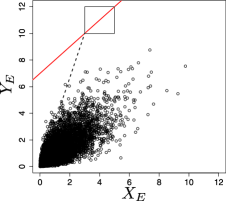
Figure 1: Bivariate normal data with dependence parameter $\rho=0.8$ on exponential margins. The line parallel to the diagonal represents a trajectory for extrapolation under the existing Ledford and Tawn [14] methodology; the dashed line represents a trajectory for extrapolation based upon the methodology we outline in Section 5.

In the theory of hidden regular variation, the normalization function $c(n)$, defined by limit (3), is determined by the extremal dependence structure of $(X_{P},Y_{P})$ upon fixing $\mbox{{P}}\{(X_{P}/c(n),Y_{P}/c(n))\in B\}\asymp n^{-1}$. In this paper, we explore the effects of applying different normalizations to the components and characterizing the decay rates of the associated multivariate distribution. In particular, we explore the behaviour of

$$\mbox{{P}}\bigl{(}X_{P}>n^{\beta},Y_{P}>n^{\gamma}\bigr{)}\equiv\mbox{{P}}(X_{E}>\beta\log n,Y_{E}>\gamma\log n)$$ (6)

for $(\beta,\gamma)\in\mathbb{R}^{2}_{+}\setminus\{\mathbf{0}\}$ as $n\rightarrow\infty$. This permits a generalization of the theory of Ledford and Tawn [14], which is a special case with the restriction $\beta=\gamma$. This generalization is desirable as it promotes methodology which overcomes some of the shortcomings of Ledford and Tawn [14], of which the principal drawback is the limited trajectories in which one can extrapolate. To highlight this, consider Figure 1, which shows realizations from a standard bivariate normal with dependence parameter $\rho=0.8$ on exponential margins. The solid line in the picture indicates a trajectory in which, for certain sets such as the one indicated, one would not be able to use the methodology of Ledford and Tawn [14], with empirical estimation of $\mbox{{P}}\{(X_{P},Y_{P})\in A^{\prime}\}$, to yield any non-zero estimation of a probability. A similar problem can be incurred in the methodology of Heffernan and Tawn [10], as identified by Peng and Qi [17], see Section 5. Ramos and Ledford [19] offer a parametric approach following on from Ledford and Tawn [14] which can avoid this issue. However, the use of parametric models brings concerns of mis-specification, and furthermore is only valid as an approximation on a sub-region $(u,\infty)^{2}$ for large $u$. The theory and subsequent methodology that we develop permits extrapolation upon rays in exponential margins, illustrated by the dashed line in Figure 1. As such, this substantially broadens the range of sets for which non-zero estimation is possible, whilst avoiding parametric assumptions. Our new representation, although more closely tied with the Ledford and Tawn [14] paradigm, also provides some modest links to the alternative limit theory of Heffernan and Tawn [10] and Heffernan and Resnick [9], and permits extrapolation into regions where not all components are simultaneously extreme.

The motivating philosophy behind our approach is a little different to the standard form. The usual limit theory for multivariate extremes takes a single normalization, and characterizes the ‘interesting’ (i.e., non-degenerate) limits that arise. By contrast here, we examine a whole class of different normalizations, but initially place our focus upon the asymptotic decay rate associated with each normalization. This characterization of the links between normalizations and decay rates enriches the mathematical structure behind multivariate extreme value theory and promotes novel statistical methodologies.

In Section 2, we develop the new representation and its justification. We focus here upon the link between the normalizing functions and the tail probability decay rates of the distributions. We also consider extensions to higher dimensions and associated issues. Section 3 explores extensions to bivariate limits. In Section 4, we detail more fully the links to the existing theories for asymptotically independent bivariate extremes. We provide some specific examples covering a variety of dependence structures, detailing their characterizations in each of the different extreme value models. Some possible statistical methodology is suggested and illustrated in Section 5; a concluding discussion is provided in Section 6.

2 Characterization of decay rates

2.1 Regular variation assumption

We focus on the characterization of the leading order power behaviour of expression (6) as $n\rightarrow\infty$. Following similar assumptions to Ledford and Tawn [14], we suppose that for all $(\beta,\gamma)\in\mathbb{R}^{2}_{+}\setminus\{\mathbf{0}\}$,

$$\mbox{{P}}\bigl{(}X_{P}>n^{\beta},Y_{P}>n^{\gamma}\bigr{)}=\mbox{{P}}(X_{E}>\beta\log n,Y_{E}>\gamma\log n)=L(n;\beta,\gamma)n^{-\kappa(\beta,\gamma)},$$ (7)

where $L$ is a univariate slowly varying function in $n$, $n\to\infty$, for all $(\beta,\gamma)\in\mathbb{R}^{2}_{+}\setminus\{\mathbf{0}\}$, and the function $\kappa(\beta,\gamma)>0$ maps the different marginal growth rates to the joint tail decay rate. Equation (7) implies that $\mbox{{P}}(X_{P}>n^{\beta},Y_{P}>n^{\gamma})$ is a regularly varying function at infinity of index $-\kappa(\beta,\gamma)$.

2.2 Consequences of the assumption

The index of regular variation

The function $\kappa$ is the key quantity in determining the behaviour of expression (7) as $n\rightarrow\infty$. We now explore some of its properties. By the regular variation assumption (7), it follows (e.g., Resnick [22], Proposition 2.6(i)) that

$$\kappa(\beta,\gamma)=-\lim_{n\rightarrow\infty}\log\mbox{{P}}\bigl{(}X_{P}>n^{\beta},Y_{P}>n^{\gamma}\bigr{)}/\log n.$$ (8)

Property 1

$\kappa$ is homogeneous of order 1.

Proof.

Take $h>0$. Then

$$\kappa(h\beta,h\gamma) = -\lim_{n\rightarrow\infty}\log\mbox{{P}}\bigl{(}X_{P}>n^{h\beta},Y_{P}>n^{h\gamma}\bigr{)}/\log n$$

$$= -h\lim_{n\rightarrow\infty}\log\mbox{{P}}\bigl{(}X_{P}>n^{h\beta},Y_{P}>n^{h\gamma}\bigr{)}/(h\log n)$$

$$= h\kappa(\beta,\gamma).$$

∎

Property 2

$\kappa$ is a non-decreasing function of each argument.

Proof.

Let $t>1$, thus $\mbox{{P}}(X_{P}>n^{t\beta},Y_{P}>n^{\gamma})\leq\mbox{{P}}(X_{P}>n^{\beta},Y_{P}>n^{\gamma})$. Following this inequality through limit (8) yields $\kappa(t\beta,\gamma)\geq\kappa(\beta,\gamma)$. ∎

Property 3

$\kappa(\beta,0)=\beta;\kappa(0,\gamma)=\gamma$.

This holds by the assumptions on the margins, that is, $\mbox{{P}}(X_{P}>n^{\beta},Y_{P}>1)=\mbox{{P}}(X_{P}>n^{\beta})=n^{-\beta}$.

Property 4

For any dependence structure, $\max\{\beta,\gamma\}\leq\kappa(\beta,\gamma)$. Under positive quadrant dependence of $(X_{P},Y_{P})$, $\kappa(\beta,\gamma)\leq\beta+\gamma$.

Proof.

Complete dependence provides the bound $\mbox{{P}}(X_{P}>n^{\beta},Y_{P}>n^{\gamma})\leq\mbox{{P}}(X_{P}>\max\{n^{\beta},\allowbreak n^{\gamma}\})$, whilst positive quadrant dependence implies $\mbox{{P}}(X_{P}>n^{\beta})\mbox{{P}}(Y_{P}>n^{\gamma})\leq\mbox{{P}}(X_{P}>n^{\beta},Y_{P}>n^{\gamma})$. Following these inequalities through limit (8) yields the result. ∎

Note that without positive quadrant dependence, $\kappa(\beta,\gamma)$ can become arbitrarily large; the bivariate normal distribution with negative dependence (Example 1 of Section 4.3) provides an example of this.

The function $\kappa$ provides information about the level of dependence between variables at sub-asymptotic levels. The homogeneity property of $\kappa$ suggests it is instructive to consider a decomposition into a radial and angular component. Define pseudo-angles $\omega:=\beta/(\beta+\gamma)$. Then $\kappa(\beta,\gamma)=(\beta+\gamma)\kappa(\omega,1-\omega)$, which motivates defining an angular dependence function $\lambda(\omega):=\kappa(\omega,1-\omega),\omega\in[0,1]$. Setting $\omega=1/2$ returns the coefficient of tail dependence $\eta$ as defined in Ledford and Tawn [13], that is, $\kappa(1,1)=2\lambda(1/2)=1/\eta$. Interestingly, the link between $1/\eta$ and the newly-defined function $\lambda$ is analogous to the link between the extremal coefficient $\theta$ and Pickands’ dependence function $A$ (Pickands [18]) of classical multivariate extremes: $\theta=2A(1/2)$, see, for example, Beirlant et al. [1].

In terms of $\lambda$, the inequalities of Property 4 read: $\max\{\omega,1-\omega\}\leq\lambda(\omega)\leq 1$. This further highlights the parallels between $\lambda$ and Pickands’ dependence function $A$, since this is one of the two characterizing features of $A$. The other feature of $A$ is convexity; convexity of $\kappa$ and $\lambda$ entails an additional dependence condition.

Proposition 0

For a random vector satisfying assumption (7), the homogeneous function $\kappa$ and angular dependence function $\lambda$ are convex if there exists $N\in\mathbb{N}$ such that for all $n>N$, and any $\delta_{1},\delta_{2},\varepsilon_{1},\varepsilon_{2}\geq 0$, $\delta_{1}+\varepsilon_{1}>0$ and $\delta_{2}+\varepsilon_{2}>0$,

$$\mbox{{P}}\bigl{\{}X_{E}>(\delta_{1}+\delta_{2})\log n,Y_{E}>(\varepsilon_{1}+\varepsilon_{2})\log n\bigr{\}}$$

(9)

$$\quad\geq\mbox{{P}}(X_{E}>\delta_{1}\log n,Y_{E}>\varepsilon_{1}\log n)\mbox{{P}}(X_{E}>\delta_{2}\log n,Y_{E}>\varepsilon_{2}\log n).$$

Conversely if $\kappa,\lambda$ are strictly convex, then for each such $\delta_{1},\delta_{2},\varepsilon_{1},\varepsilon_{2}$, there exists $N(\delta_{1},\delta_{2},\allowbreak\varepsilon_{1},\varepsilon_{2})\in\mathbb{N}$ such that for all $n>N(\delta_{1},\delta_{2},\varepsilon_{1},\varepsilon_{2})$, inequality (1) holds.

Proof.

Suppose inequality (1) holds. By taking log of each side of (1), and applying (8), we deduce $\kappa(\delta_{1}+\delta_{2},\varepsilon_{1}+\varepsilon_{2})\leq\kappa(\delta_{1},\varepsilon_{1})+\kappa(\delta_{2},\varepsilon_{2})$, that is, $\kappa$ is subadditive. Homogeneous order 1 functions defined on convex cones are convex if and only if they are subadditive (e.g., Niculescu and Persson [16], Lemma 3.6.1). In terms of $\lambda$, we have

$$(\delta_{1}+\delta_{2}+\varepsilon_{1}+\varepsilon_{2})\lambda\biggl{(}\frac{\delta_{1}+\delta_{2}}{\delta_{1}+\delta_{2}+\varepsilon_{1}+\varepsilon_{2}}\biggr{)}\leq(\delta_{1}+\varepsilon_{1})\lambda\biggl{(}\frac{\delta_{1}}{\delta_{1}+\varepsilon_{1}}\biggr{)}+(\delta_{2}+\varepsilon_{2})\lambda\biggl{(}\frac{\delta_{2}}{\delta_{2}+\varepsilon_{2}}\biggr{)}.$$

Dividing through by $\delta_{1}+\delta_{2}+\varepsilon_{1}+\varepsilon_{2}$ and noting the relation between the arguments of $\lambda$ yields convexity. Conversely, if $\lambda$ is strictly convex then $\kappa$ is strictly subadditive. Showing that (1) holds for all $n>N(\delta_{1},\delta_{2},\varepsilon_{1},\varepsilon_{2})$, is equivalent to showing

$$n^{\kappa(\delta_{1},\varepsilon_{1})+\kappa(\delta_{2},\varepsilon_{2})-\kappa(\delta_{1}+\delta_{2},\varepsilon_{1}+\varepsilon_{2})}\geq L(n;\delta_{1},\varepsilon_{1})L(n;\delta_{2},\varepsilon_{2})/L(n;\delta_{1}+\delta_{2},\varepsilon_{1}+\varepsilon_{2}).$$ (10)

Taking log of each side of (10) and dividing by $\log n$ gives $\kappa(\delta_{1},\varepsilon_{1})+\kappa(\delta_{2},\varepsilon_{2})-\kappa(\delta_{1}+\delta_{2},\varepsilon_{1}+\varepsilon_{2})>0$ on the LHS and $\log\{L(n;\delta_{1},\varepsilon_{1})L(n;\delta_{2},\varepsilon_{2})/L(n;\delta_{1}+\delta_{2},\varepsilon_{1}+\varepsilon_{2})\}/\log n\to 0$ as $n\to\infty$ on the RHS. Therefore, there exists $N(\delta_{1},\delta_{2},\varepsilon_{1},\varepsilon_{2})\in\mathbb{N}$ such that for all $n>N(\delta_{1},\delta_{2},\varepsilon_{1},\varepsilon_{2})$ (1) holds. ∎

The inequality (1) has an interpretation in terms of an existing dependence condition given in Joe [12]: the random vector $(X_{E},Y_{E})$ gives rise to a convex $\kappa$ if asymptotically, the conditional vector $(X_{E},Y_{E})|(X_{E}>\delta_{1}\log n,Y_{E}>\varepsilon_{1}\log n)$ is more concordant or more positively quadrant dependent, as $n\rightarrow\infty$, than the unconditional vector $(X_{E},Y_{E})$. The majority of the examples in Section 4.3 have a convex $\lambda$; the bivariate normal distribution with negative dependence provides an example of a concave $\lambda$. However, convexity is different in general to positive quadrant dependence of $(X_{E},Y_{E})$, which only provides the upper bound $\lambda(\omega)\leq 1$. In a similar manner to Proposition 1, we have a partial converse: $\lambda(\omega)<1$, $\omega\in(0,1)$, implies that for each $\omega\in(0,1)$, there exists some $N(\omega)\in\mathbb{N}$ such that for all $n>N(\omega)$,

$$L(n;\omega,1-\omega)n^{-\lambda(\omega)}\geq n^{-\omega+(1-\omega)}=n^{-1},$$

that is, positive quadrant dependence for some sufficiently large $n>N(\omega)$.

The slowly varying function

For estimation of extreme probabilities, it is the index $\lambda(\omega)$ which principally controls the joint tail probability decay rate. However, the behaviour of the slowly varying function $L$ does affect the estimation of $\lambda$ (see Section 5). Owing to the assumptions of our representation, $L$ must satisfy certain properties. One is a marginal property: $L(n;0,\gamma)=L(n;\beta,0)=1$, by the assumption of Pareto margins. This tells us that $L$ is identically constant iff $L\equiv 1$. A further homogeneity property arises from the assumption that representation (7) holds for any $(\beta,\gamma)\in\mathbb{R}^{2}_{+}\setminus\{\mathbf{0}\}$. For $h>0$, $L(n^{h};\beta,\gamma)=L(n;h\beta,h\gamma)$, showing we can also specify to the case $\beta+\gamma=1$, defining $L^{*}(n;\omega):=L(n;\omega,1-\omega)$.

2.3 Generalization of scaling functions

For any $\omega\in[0,1]$, define the transformation $T_{\omega}\mathchoice{\nobreak\,\colon}{\nobreak\,\colon}{\nobreak\,\colon\;}{\nobreak\,\colon\;}[1,\infty)\mapsto[1,\infty)^{2}$ by $T_{\omega}(x)=(x^{\omega},x^{1-\omega})$, and denote the joint survivor function of $(X_{P},Y_{P})$ by $\bar{F}\mathchoice{\nobreak\,\colon}{\nobreak\,\colon}{\nobreak\,\colon\;}{\nobreak\,\colon\;}[1,\infty)^{2}\mapsto(0,1]$. Assumption (7) can be written

$$\bar{F}\circ T_{\omega}\in RV_{-\lambda(\omega)}\qquad\forall\omega\in[0,1],$$

where $RV_{\rho}$ stands for the class of univariate regularly varying functions at infinity with index $\rho$ (see, e.g., Resnick [21, 22]).

We can generalize the scaling functions from exact power law scaling to regularly varying functions. Define $\bar{H}_{\omega}(n):=\bar{F}\circ T_{\omega}(n)$, which is the survivor function of the random variable $\min\{X_{P}^{1/\omega},Y_{P}^{1/(1-\omega)}\}$, and hence monotonic. For $\omega=0$, we define $\min\{X_{P}^{1/0},Y_{P}^{1/1}\}=:Y_{P}$, and similarly for $\omega=1$. Then we may define a non-decreasing function $b(n)\rightarrow\infty$ such that $\bar{H}_{\omega}(b(n))\sim n^{-\lambda(\omega)}$, $n\to\infty$, by taking $b(n)=(1/\bar{H}_{\omega})^{\leftarrow}(n^{\lambda(\omega)})$, with $(1/\bar{H}_{\omega})^{\leftarrow}$ the inverse of $1/\bar{H}_{\omega}$. By Proposition 2.6(iv) and (v) of Resnick [22], we can deduce $b(n)\in RV_{1}$, and thus as $n\to\infty$,

$$\bar{F}\circ T_{\omega}\circ b(n)=\mbox{{P}}\bigl{(}X_{P}>b(n)^{\omega},Y_{P}>b(n)^{1-\omega}\bigr{)}\sim n^{-\lambda(\omega)}.$$

2.4 Higher dimensions, strong and weak joint tail dependence

The extension to higher dimensions involves a generalized notion of asymptotic dependence and asymptotic independence. Let $\mathbf{X}$ be a random $d$-vector with marginal distribution functions $F_{X_{1}},\ldots,F_{X_{d}}$. We define the notion of $d$-dimensional joint tail dependence through the limit

$$\chi(D)=\lim_{u\rightarrow 1}\mbox{{P}}\bigl{\{}F_{X_{j}}(X_{j})>u,\forall j\in D|F_{X_{1}}(X_{1})>u\bigr{\}}$$ (11)

for $D=\{1,\ldots,d\}$. The cases $\chi(D)>0$ and $\chi(D)=0$ define, respectively, strong joint tail dependence and weak joint tail dependence of the vector. Convergence (2) extends to $d$-dimensions. For $\mathbf{X}_{P}$ a random $d$-vector with Pareto margins, we have $n\mbox{{P}}(\mathbf{X}_{P}/n\in\cdot)\stackrel{{\scriptstyle v}}{{\rightarrow}}\mu(\cdot)$ on $[0,\infty]^{d}\setminus\{\mathbf{0}\}$. The homogeneous order $-1$ measure $\mu$ has mass on the particular subcone $(0,\infty]^{d}\subset[0,\infty]^{d}\setminus\{\mathbf{0}\}$ only if the vector exhibits $d$-dimensional strong joint tail dependence. For $d>2$, weak joint tail dependence does not imply that the limiting normalized componentwise maxima would be mutually independent, though the converse is true. For $d=2$, weak joint tail dependence is equivalent to asymptotic independence. In addition, if $\chi(\{i,j\})=0$ for all pairs $i,j\in D$ the limiting normalized componentwise maxima would be mutually independent.

With a slight change of notation, let $\mathbf{X}_{E}=\log\mathbf{X}_{P}$ be $d$-vectors and $\bolds{\beta}=(\beta_{1},\ldots,\beta_{d})$ be the vector replacing $(\beta,\gamma)$ in two dimensions. The function $\kappa$ is understood to have as many arguments as the context dictates. Applying all vector operations componentwise assume

$$\mbox{{P}}(\mathbf{X}_{E}>\bolds{\beta}\log n)=L(n;\bolds{\beta})n^{-\kappa(\bolds{\beta})}$$ (12)

with all quantities being defined analogously to the bivariate case.

Once more, we can define $\omega_{i}=\beta_{i}/\sum_{j}\beta_{j}$ so that $\bolds{\omega}=(\omega_{1},\ldots,\omega_{d})\in S_{d}:=\{\mathbf{v}\in[0,1]^{d}\mathchoice{\nobreak\,\colon}{\nobreak\,\colon}{\nobreak\,\colon\;}{\nobreak\,\colon\;}\allowbreak\sum_{i=1}^{d}v_{i}=1\}$ and the function $\lambda(\omega_{1},\ldots,\omega_{d-1}):=\kappa(\bolds{\omega})$. The previously outlined properties of $\kappa$ and $\lambda$ hold just as in the bivariate case; for Property 4 the upper bound follows from extending the assumption to positive upper orthant dependence (Joe [12]), other extensions are clear. In addition, we have a consistency condition as we move across dimensions:

$$\kappa(\beta_{1},\ldots,\beta_{d})\geq\kappa(\beta_{1},\ldots,\beta_{d-1},0)=\kappa(\beta_{1},\ldots,\beta_{d-1}).$$

For a $d$-dimensional random vector, a summary of the limiting dependence structure of the full vector is given by the values of $\chi(C)$, for all possible $C\subseteq D$. If $\chi(C)>0$ then $\mu(B)>0$ for $B$ some Borel subset of $\mathop{\mbox{{$\!\times$}}}_{i=1}^{d}(0,\infty]^{I(i\in C)}[0,\infty]^{I(i\notin C)}$, with $I$ the indicator function and $\mathop{\mbox{{$\!\times$}}}_{i=1}^{d}$ representing Cartesian product of sets (e.g., if $D=\{1,2,3\}$, $C=\{1,3\}$, the notation should be interpreted to mean $(0,\infty]\times[0,\infty]\times(0,\infty]$). Otherwise, $\chi(C)=0$ implies $\mu(B)=0$ for all Borel $B$ on the same space, and hence the vague convergence in (2) provides no interesting theoretical discrimination for the dependence structure of the subset indexed by $C$. In this sense, we have a boundary case of the limit measure $\mu$. By contrast, $\kappa$ can still provide some discrimination between different levels of sub-asymptotic dependence amongst the variables indexed by $C$.

Conversely, when $\chi(C)>0$, this strong joint tail dependence forms a boundary case in the asymptotic theory suitable for analyzing weak joint tail dependence. We cannot avoid this easily since we have the dichotomy that the joint survivor function $\bar{F}$ of $\mathbf{X}_{P}$ either decays at the same rate as the marginal survivor functions (strong joint tail dependence) or faster than the marginal rate (weak joint tail dependence). As a consequence here, we find that for any distribution satisfying (12) and exhibiting $d$-dimensional strong joint tail dependence, $\lambda(\omega_{1},\ldots,\omega_{d-1})=\max_{1\leq i\leq d}\{\omega_{i}\}$ (see Proposition 2) and we only have different forms of $\lambda$ describing different forms of weak joint tail dependence.

Proposition 0

Let $\mathbf{X}_{P}$ satisfy (12). If $\mathbf{X}_{P}$ exhibits $d$-dimensional strong joint tail dependence, that is, $\chi(D)>0$, then $\kappa(\beta_{1},\ldots,\beta_{d})=\max_{1\leq i\leq d}\{\beta_{i}\}$.

Proof.

Because $\chi(D)>0$, by definition (11), we have for $\beta_{1}>0$

$$\lim_{n\rightarrow\infty}\mbox{{P}}(X_{P,2}>n,\ldots,X_{P,d}>n|X_{P,1}>n)$$

$$\quad=\lim_{n\rightarrow\infty}\mbox{{P}}\bigl{(}X_{P,2}>n^{\beta_{1}},\ldots,X_{P,d}>n^{\beta_{1}}|X_{P,1}>n^{\beta_{1}}\bigr{)}=\chi(D)>0.$$

Without loss of generality, assume $\beta_{1}=\max_{1\leq i\leq d}\{\beta_{i}\}$. Then we also have

$$1 \geq \mbox{{P}}\bigl{(}X_{P,2}>n^{\beta_{2}},\ldots,X_{P,d}>n^{\beta_{d}}|X_{P,1}>n^{\beta_{1}}\bigr{)}$$

$$\geq \mbox{{P}}\bigl{(}X_{P,2}>n^{\beta_{1}},\ldots,X_{P,d}>n^{\beta_{1}}|X_{P,1}>n^{\beta_{1}}\bigr{)}\rightarrow\chi(D)$$

as $n\rightarrow\infty$. Hence, $\mbox{{P}}(X_{P,1}>n^{\beta_{1}},X_{P,2}>n^{\beta_{2}},\ldots,X_{P,d}>n^{\beta_{d}})\asymp n^{-\beta_{1}}$, as $n\to\infty$, that is, $\kappa(\beta_{1},\ldots,\beta_{d})=\max_{1\leq i\leq d}\{\beta_{i}\}$. ∎

In practice as $d$ grows it becomes more likely that a scenario will arise for which some sets $C\subseteq D$ yield $\chi(C)=0$ and some yield $\chi(C)>0$, and as such, tools from both dependence paradigms will be useful. For relative simplicity of exposition, we return the focus to the bivariate case for the rest of the paper.

3 Bivariate limits

In this section, we detail some results concerning bivariate limits, initially by conditioning upon the event that $(X_{P},Y_{P})\in(n^{\omega},\infty)\times(n^{1-\omega},\infty)$.

3.1 Assumption

Consider, for $x,y\geq 1$, $\mbox{{P}}(X_{P}>n^{\omega}x,Y_{P}>n^{1-\omega}y|X_{P}>n^{\omega},Y_{P}>n^{1-\omega})$; under assumption (7) this is given by

$$\frac{L(n;\omega+{\log x}/{\log n},1-\omega+{\log y}/{\log n})}{L(n;\omega,1-\omega)}$$

(13)

$$\quad{}\times\exp\biggl{[}\log n\biggl{\{}\kappa(\omega,1-\omega)-\kappa\biggl{(}\omega+\frac{\log x}{\log n},1-\omega+\frac{\log y}{\log n}\biggr{)}\biggr{\}}\biggr{]}.$$

We shall initially explore the limiting behaviour of this expression under the assumption that $\kappa$ is differentiable and that

$$\lim_{n\rightarrow\infty}\frac{L(n;\omega+{\log x}/{\log n},1-\omega+{\log y}/{\log n})}{L(n;\omega,1-\omega)}=1.$$ (14)

Such assumptions are smoothness conditions on the behaviour of the joint distributional tail over different $\omega$. They are analogous to supposing ray independence of the Ledford and Tawn [14] paradigm; a condition which actually holds very widely including for all of the asymptotically independent examples of the Ledford and Tawn [14] paper. The development under these assumptions will permit us to observe how a generalized notion of multivariate regular variation is possible at the end of the section.

3.2 Conditional limits under the assumption

Since we assume that $\kappa$ is differentiable at the point $\bolds{\omega}:=(\omega,1-\omega)$, then

$$\lim_{n\rightarrow\infty}\log n\biggl{[}\kappa(\omega,1-\omega)-\kappa\biggl{(}\omega+\frac{\log x}{\log n},1-\omega+\frac{\log y}{\log n}\biggr{)}\biggr{]}=-\nabla\kappa(\omega,1-\omega)\cdot(\log x,\log y)^{T}$$

with $\nabla\kappa$ the gradient vector of $\kappa$. Therefore, the conditional probability limit from equation (3.1) is

$$\exp\bigl{\{}-\nabla\kappa(\omega,1-\omega)\cdot(\log x,\log y)^{T}\bigr{\}}=x^{-\kappa_{1}(\omega)}y^{-\kappa_{2}(\omega)},$$ (15)

that is, independent Pareto variables with shape parameters

$$\bigl{\{}\kappa_{1}(\omega),\kappa_{2}(\omega)\bigr{\}}:=\biggl{(}\frac{\partial\kappa}{\partial\beta},\frac{\partial\kappa}{\partial\gamma}\biggr{)}\bigg{|}_{(\omega,1-\omega)}=\bigl{\{}\lambda(\omega)+(1-\omega)\lambda^{\prime}(\omega),\lambda(\omega)-\omega\lambda^{\prime}(\omega)\bigr{\}}.$$

By Property 2, it is clear that $\kappa_{1}(\omega),\kappa_{2}(\omega)\geq 0$. In exponential margins, for $x,y\geq 0$, this reads

$$\lim_{n\rightarrow\infty}\frac{\mbox{{P}}\{X_{E}-\omega\log n>x,Y_{E}-(1-\omega)\log n>y\}}{\mbox{{P}}\{X_{E}>\omega\log n,Y_{E}>(1-\omega)\log n\}} = \exp\bigl{\{}-\nabla\kappa(\omega,1-\omega)\cdot(x,y)\bigr{\}}\quad$$

$$= \exp\bigl{\{}-\kappa_{1}(\omega)x-\kappa_{2}(\omega)y\bigr{\}}.$$

Although stochastic independence of the conditioned normalized variables arises in the limit, limits (15) and (3.2) are interpretable in terms of the original degree of dependence at the finite level. This can be observed by the relation $\kappa_{1}(\omega)=\kappa_{2}(\omega)+\lambda^{\prime}(\omega)$. As the variables become independent, $\lambda(\omega)$ and $\lambda^{\prime}(\omega)$ approach 1 and 0, respectively, thus $\kappa_{1}(\omega)$ and $\kappa_{2}(\omega)$ approach equality. As dependence increases, then $\kappa_{1}(\omega)$ decreases relative to $\kappa_{2}(\omega)$ for $\omega<1/2$, and vice versa.

The boundary case of asymptotic dependence has $\kappa_{1}(\omega)=0$ and $\lambda^{\prime}(\omega)=-1$ for $\omega<1/2$ and $\kappa_{2}(\omega)=0$ and $\lambda^{\prime}(\omega)=1$ for $\omega>1/2$. Under asymptotic dependence, the function $\lambda(\omega)=\max\{\omega,1-\omega\}$ is not differentiable at $\omega=1/2$, and the above limits (15) and (3.2) do not hold on this line. However, when $\omega\neq 1/2$, we can still get the conditional limit from (15) to be $x^{-1}I(\omega>1/2)+y^{-1}I(\omega<1/2)$. When $\omega=1/2$, standard theory for asymptotically dependent distributions provides that the limit is $\{x^{-1}+y^{-1}-V(x,y)\}/\{2-V(1,1)\}$, where $V(x,y):=\mu(\{[0,x]\times[0,y]\}^{c})$ for the appropriate limiting measure $\mu$ in convergence (2).

The asymptotic dependence case highlights some subtleties that occur when the assumptions of differentiable $\kappa$ and assumption (14) break down. In this case, the function $L$ inherits additional structure at the point where $\kappa$ is not differentiable, and classical multivariate regular variation conditions become the appropriate tools for analysis.

3.3 Multivariate regular variation

The weak convergence of probability measures given by limit (15) can be expressed more generally as

$$\mbox{{P}}\biggl{\{}\biggl{(}\frac{X_{P}}{n^{\omega}},\frac{Y_{P}}{n^{1-\omega}}\biggr{)}\in\cdot\bigg{|}\biggl{(}\frac{X_{P}}{n^{\omega}},\frac{Y_{P}}{n^{1-\omega}}\biggr{)}\in[1,\infty)^{2}\biggr{\}}\stackrel{{\scriptstyle w}}{{\rightarrow}}\pi(\cdot;\omega)$$ (17)

on $(1,\infty)^{2}$ as $n\rightarrow\infty$, with the limit measure $\pi(\cdot;\omega)$ homogeneous of order $-\{\kappa_{1}(\omega)+\kappa_{2}(\omega)\}$. This reveals an alternative non-standard type of regular variation condition. A function $q$ is (standard) multivariate regularly varying with index $\rho\in\mathbb{R}$ and limit function $\Lambda$ if $\lim_{t\rightarrow\infty}q(t\mathbf{x})/q(t\mathbf{1})=\Lambda(\mathbf{x})$, $\mathbf{x}\in\mathbb{R}^{d}_{+}$, the function $q(t\mathbf{1})=:Q(t)\in RV_{\rho}$, is univariate regularly varying, and $\Lambda(c\mathbf{x})=c^{\rho}\Lambda(\mathbf{x})$, $c>0$. The common scaling $t\in RV_{1}$ can be replaced by any common scaling $b(t)\in RV_{\alpha}$, $\alpha>0$, yielding an unchanged limit function and $Q\circ b(t)\in RV_{\rho\alpha}$. In limit (17) however, different scalings are applied to each component, in the classes $RV_{\omega}$ and $RV_{1-\omega}$, $Q\circ T_{\omega}(t)\in RV_{-\lambda(\omega)}$, and the order of homogeneity of the limit measure is $-\{\kappa_{1}(\omega)+\kappa_{2}(\omega)\}$. When $\omega=1/2$, the common scaling returns standard multivariate regular variation since the limit measure is homogeneous of order $-\{\kappa_{1}(1/2)+\kappa_{2}(1/2)\}=-\kappa(1,1)=-2\lambda(1/2)=-1/\eta$. Note this is a different form of non-standard regular variation to that given in Resnick [22], as there the non-equal scalings are due to non-equal margins.

Limit (17) provides an asymptotic link between the probabilities of lying in Borel sets $B\subset[1,\infty)^{2}$ where each component is scaled by $(n^{\omega},n^{1-\omega})$ as

$$\mbox{{P}}\biggl{\{}\biggl{(}\frac{X_{P}}{n^{\omega}},\frac{Y_{P}}{n^{1-\omega}}\biggr{)}\in\bigl{(}t^{\omega},t^{1-\omega}\bigr{)}B\biggr{\}}\sim t^{-\lambda(\omega)}\mbox{{P}}\biggl{\{}\biggl{(}\frac{X_{P}}{n^{\omega}},\frac{Y_{P}}{n^{1-\omega}}\biggr{)}\in B\biggr{\}}$$

as $n\rightarrow\infty$, $t>1$, with vector arithmetic applied componentwise. This follows since $\omega\kappa_{1}(\omega)+(1-\omega)\kappa_{2}(\omega)=\kappa(\omega,1-\omega)=\lambda(\omega)$ by homogeneity. Together with the corresponding relation in exponential margins, this provides the analogous equations to (1).

By the form of limit (17), we observe that this can be modified to standard multivariate regular variation. Define the bijective map $U_{\omega}\mathchoice{\nobreak\,\colon}{\nobreak\,\colon}{\nobreak\,\colon\;}{\nobreak\,\colon\;}(1,\infty)^{2}\mapsto(1,\infty)^{2}$ by $U_{\omega}(x,y)=(x^{\omega},y^{1-\omega})$, for any fixed $\omega\in(0,1)$. Then $\bar{F}\circ U_{\omega}$ is multivariate regularly varying of index $-\lambda(\omega)$. Equivalently we can think of this as standard multivariate regular variation of the law of the random vector $U_{\omega}^{\leftarrow}(X_{P},Y_{P})=(X_{P}^{1/\omega},Y_{P}^{1/(1-\omega)})$, $\omega\in(0,1)$. In place of convergence (17), we can thus consider,

$$\mbox{{P}}\bigl{\{}U_{\omega}^{\leftarrow}(X_{P},Y_{P})/n\in\cdot|U_{\omega}^{\leftarrow}(X_{P},Y_{P})/n\in[1,\infty)^{2}\bigr{\}}\stackrel{{\scriptstyle w}}{{\rightarrow}}\pi^{*}(\cdot;\omega)$$ (18)

on $(1,\infty)^{2}$, where for Borel $B\subset(1,\infty)^{2}$, $c>0$, $\pi^{*}(cB;\omega)=c^{-\lambda(\omega)}\pi^{*}(B;\omega)$. When $\omega=1/2$, this is standard multivariate regular variation, and does not therefore require the assumptions of differentiable $\kappa$ and (14). Consequently, (18) provides a general multivariate asymptotic characterization for both asymptotically dependent and asymptotically independent random vectors, where the structure rests in $\pi^{*}(\cdot;1/2)$ under asymptotic dependence, and the combination of $\lambda(\omega)$ and $\pi^{*}(\cdot;\omega)$ under asymptotic independence.

As in the univariate case, the scaling functions can be generalized from exact powers of $n$ to regularly varying functions. Under our current assumptions, we can find $a(n)\in RV_{1/\lambda(\omega)}$ such that for Borel $B\subset(1,\infty)^{2}$,

$$\lim_{n\to\infty}n\mbox{{P}}\bigl{\{}U_{\omega}^{\leftarrow}(X_{P},Y_{P})/a(n)\in B\bigr{\}}=\pi^{*}(B;\omega)$$

with $\pi^{*}(\partial B)=0$ and $\pi^{*}$ as given in convergence (18). This follows by defining $a(n)=(1/\bar{H}_{\omega})^{\leftarrow}(n)$, as in Section 2.3, and using the assumptions of Section 3.1 on $L$ and $\kappa$, or standard multivariate regular variation assumptions.

4 Connections to existing theory for asymptotic independence

In this section, we detail more carefully the connections between our representation (7) and the existing theories which permit non-trivial treatment of asymptotic independence. Specifically, these are the theories introduced by Ledford and Tawn [14] and Heffernan and Tawn [10]. These representations were originally phrased in terms of standard Fréchet and standard Gumbel margins, respectively. Here, we continue to use the asymptotically equivalent standard Pareto and exponential margins.

4.1 Coefficient of tail dependence

The assumption of Ledford and Tawn [14] is given by (4). Supposing that $\kappa$ is differentiable then the results of Section 3 allow us to write

$$\mbox{{P}}\bigl{(}X_{P}>n^{\omega}x,Y_{P}>n^{1-\omega}y\bigr{)}$$

(19)

$$\quad=n^{-\lambda(\omega)}x^{-\kappa_{1}(\omega)}y^{-\kappa_{2}(\omega)}L(n;\omega+\log x/\log n,1-\omega+\log y/\log n)$$

for $x,y\geq 1$ as $n\rightarrow\infty$. Setting $\omega=1/2$ in equation (4.1) returns the set-up of equation (4). From this, we see that the representations are equivalent when $c_{1}=\kappa_{1}(1/2)=\lambda(1/2)+\lambda^{\prime}(1/2)/2$, $c_{2}=\kappa_{2}(1/2)=\lambda(1/2)-\lambda^{\prime}(1/2)/2$ and $\mathcal{L}(nx,ny)\sim L(n;1+\log x/\log n,1+\log y/\log n)$, $n\to\infty$.

Ramos and Ledford [19] introduced an expanded characterization of the Ledford and Tawn [14] framework. Similarly to Section 3, they consider convergence of measures $\mbox{{P}}(X_{F}>nx,Y_{F}>ny|X_{F}>n,Y_{F}>n)$, with $(X_{F},Y_{F})$ marginally standard Fréchet, however without the condition (14). This entails the possibility of more structure in the limit measure, and is a more natural idea under equal marginal growth rates, where any non-constant limit in equation (14) would be homogeneous of order 0. Equation (18) has the Ramos and Ledford [19] assumption as a special case. However, their focus is on developing consequences of the multivariate regular variation condition under common scaling of the margins, whilst our focus remains on consequences of generalizing the scaling.

4.2 Conditioned limit theory

Heffernan and Tawn [10] generated a limit theory for the distribution of a variable $X$, suitably normalized, conditional upon the concomitant variable, $Y$, being extreme. In standard Gumbel margins, they considered non-degenerate limits of

$$\mbox{{P}}\bigl{(}\bigl{\{}X_{G}-b(y)\bigr{\}}/a(y)\leq x|Y_{G}=y\bigr{)}$$ (20)

as $y\rightarrow\infty$. The normalizing functions $a,b$ satisfy $a(y)>0$, $b(y)\leq y$, and give unique limit distributions up to type (see Heffernan and Tawn [10], Theorem 1). Precise forms of $a,b$ are stated on the understanding that modifications which do not change the type of limit distribution are allowable. In this limit theory, asymptotic dependence is once more a boundary case requiring the normalizations $a(y)=1$ and $b(y)=y$. Formulation (20) was elaborated on by Heffernan and Resnick [9], who described limit theory for both

$$\mbox{{P}}\bigl{(}\bigl{\{}X_{E}-b(\log n)\bigr{\}}/a(\log n)\leq x|Y_{E}>\log n\bigr{)}$$

(21)

$$\mbox{{P}}\bigl{(}\bigl{\{}X_{E}-b(Y_{E})\bigr{\}}/a(Y_{E})\leq x|Y_{E}>\log n\bigr{)}$$

as $n\rightarrow\infty$. The formulation of Heffernan and Resnick [9] is in fact slightly more general as the marginal distribution of the $X$ variable is left unspecified, however it is convenient here to suppose a particular form.

It is possible to draw some modest links between our representation and the limits in (4.2). However, the full structure of the function $L$ in representation (7) across different $\beta,\gamma$ is key in determining the limits of (4.2). By fixing $(\beta,\gamma)\in\mathbb{R}_{+}^{2}\setminus\{\mathbf{0}\}$, and considering asymptotics in $n$, then any slowly varying function $L_{1}(n;\beta,\gamma)\sim L(n;\beta,\gamma)$, $n\to\infty$, suffices for our calculations: this highlights the difference between the theories.

Under assumption (7) and with $\gamma=1$,

$$\mbox{{P}}(X_{E}>\beta\log n|Y_{E}>\log n) = L(n;\beta,1)n^{1-\kappa(\beta,1)}$$

$$= L(n;\beta,1)\exp\bigl{[}\bigl{\{}1-\kappa(\beta,1)\bigr{\}}\log n\bigr{]}$$

as $n\rightarrow\infty$. If we view the $\log n$ in the first argument of the conditional probability (4.2) as being part of the conditioning variable, then we want to find $\beta=\beta(n,x)$ such that $\beta(n,x)\log n=a(\log n)x+b(\log n)$ gives a non-degenerate limit in $x$ of equation (4.2) as $n\rightarrow\infty$. That is, we are searching for the functions $a,b,k$ such that

$$\lim_{n\rightarrow\infty}\mbox{{P}}\bigl{(}\bigl{\{}X_{E}-b(\log n)\bigr{\}}/a(\log n)>x|Y_{E}>\log n\bigr{)}=\exp\bigl{\{}-k(x)\bigr{\}},$$ (23)

defines a valid survivor function. Supposing that $\lim_{n\rightarrow\infty}\beta(n,x)=0$, one can observe that the only simple link between the two theories arises when $L\equiv 1$, since by the marginal condition $L(n;\beta,0)=L(n;0,\gamma)=1$. In this case, equation (4.2) shows that the components required for the limit (23) satisfy the relation that

$$\kappa\bigl{(}\beta(n,x),1\bigr{)}-1\sim k(x)/\log n$$ (24)

as $n\rightarrow\infty$. When $L\not\equiv 1$, then the first order theory for $\mbox{{P}}(X_{E}>\beta\log n,Y_{E}>\gamma\log n)$ that is the focus of our work is insufficient to yield the full limit distribution of equation (23). Example 3 of the following section provides an illustration of this.

4.3 Examples

Below we provide examples to illustrate the theory developed and the links with existing representations. In each case, we provide the copula, $C(u,v)$, of the distribution (i.e., the joint distribution function on standard uniform margins) and the asymptotic joint survivor function (7) on exponential margins. Table 1 summarizes the previously defined quantities $\kappa(\beta,\gamma)$;

Table 1: Summary of important theoretical quantities for representations of Examples 1–5 under the theory of the current paper, Ledford and Tawn [13] and Heffernan and Tawn [10]/Heffernan and Resnick [9]

Example	$\kappa(\beta,\gamma)$	$\eta$	$a(\log n)$	$b(\log n)$	$\exp\{-k(x)\}$
1	(a) $\frac{\beta+\gamma-2\rho(\beta\gamma)^{1/2}}{1-\rho^{2}}$;	$(1+\rho)/2$	$(2\rho^{2}\log n)^{1/2}$tb	$\rho^{2}\log n$tb	$1-\Phi\bigl{\{}\frac{x}{(1-\rho^{2})^{1/2}}\bigr{\}}$
	(b) $\max\{\beta,\gamma\}$
2	$V(1/\beta,1/\gamma)$	$1/V(1,1)$	ta	ta	ta
3	$\beta+\gamma$	$1/2$	$1$	$0$	$e^{-x}[1+\alpha(1-e^{-x})]$
4	$\max\{\beta,\gamma\}$	$1$	$1$	$\log n$	$e^{-x}[1+e^{x}-V(1,e^{-x})]$
5	$\max\{\beta,\gamma\}$	$1$	$1$	$\log n$	$[e^{x/\alpha}+1]^{-\alpha}$

[$*$]taDenotes that the explicit form depends upon $V$. [$\dagger$]tbDenotes for $\rho>0$. Example 1(a): $\rho^{2}<\min\{\beta/\gamma,\gamma/\beta\}$ or $\rho<0$ and $\min\{\beta,\gamma\}>0$; Example 1(b): all other $\rho$.

$\eta$; $a(\log n),b(\log n)$; and $\exp\{-k(x)\}$. Detailed derivations are provided for two interesting examples: the bivariate normal, and the inverted bivariate extreme value distribution. Other bivariate examples are stated more briefly. We additionally present a trivariate example for which $\chi(\{1,2,3\})=0$ but some $\chi(\{i,j\})>0$ to illustrate behaviour both across dimensions and extremal dependence classes.

Example 1 ((Bivariate normal distribution)).

$$C(u,v)=\Phi_{2}\bigl{(}\Phi^{-1}(u),\Phi^{-1}(v);\rho\bigr{)},\qquad\rho\in[-1,1],$$

with $\Phi$ the standard normal distribution function and $\Phi_{2}(\cdot,\cdot;\rho)$ the standard bivariate normal distribution function. Denote also by $\phi_{2}$ the associated joint density. The survivor function in this case is defined only via an integral, however an asymptotic expansion yields $\kappa$ and the leading order term of $L$. Let $(X_{N},Y_{N})$ denote the vector on standard normal margins. Interest lies in $\mbox{{P}}(X_{E}>\beta\log n,Y_{E}>\gamma\log n)=\mbox{{P}}\{X_{N}>\Phi^{-1}(1-n^{-\beta}),Y_{N}>\Phi^{-1}(1-n^{-\gamma})\}$. Let $x_{\beta}:=\Phi^{-1}(1-n^{-\beta})$; $x_{\gamma}:=\Phi^{-1}(1-n^{-\gamma})$. Then as $n\to\infty$

$$x_{\beta}=(2\beta\log n)^{1/2}-\bigl{(}\log\log n^{\beta}+\log 4\uppi\bigr{)}/\bigl{\{}{2(2\beta\log n)^{1/2}}\bigr{\}}+\mathrm{o}\bigl{\{}(\log n)^{-1/2}\bigr{\}}$$

and similarly $x_{\gamma}$, thus $x_{\beta}\sim(2\beta\log n)^{1/2}$, $x_{\gamma}\sim(2\gamma\log n)^{1/2}$, and hence $x_{\beta}\sim(\beta/\gamma)^{1/2}x_{\gamma}$ as $n\rightarrow\infty$ for $\beta,\gamma>0$. Bounds on the multivariate Mills’ ratio $\mbox{{P}}(X_{N}>x_{\beta},Y_{N}>x_{\gamma})/\phi_{2}(x_{\beta},\allowbreak x_{\gamma};\rho)$, obtained by Savage [24], or the asymptotic results of Ruben [23], see also Hashorva and Hüsler [7], provide that for $x_{\beta}>\rho x_{\gamma}$ and $x_{\gamma}>\rho x_{\beta}$,

$$\mbox{{P}}(X_{N}>x_{\beta},Y_{N}>x_{\gamma})\sim L_{1}(n;\beta,\gamma)n^{-\{({\beta+\gamma-2\rho(\beta\gamma)^{1/2}})/({1-\rho^{2}})\}}$$

as $n\rightarrow\infty$ with

$$L_{1}(n;\beta,\gamma) = (4\uppi\log n)^{({2\rho^{2}-\rho\{(\beta/\gamma)^{1/2}+(\gamma/\beta)^{1/2}\}})/({2(1-\rho^{2})})}$$

$${}\times\frac{\beta^{({1-\rho(\gamma/\beta)^{1/2}})/({2(1-\rho^{2})})}\gamma^{({1-\rho(\beta/\gamma)^{1/2}})/({2(1-\rho^{2})})}(1-\rho^{2})^{3/2}}{(\beta^{1/2}-\rho\gamma^{1/2})(\gamma^{1/2}-\rho\beta^{1/2})}.$$

Note that $L_{1}\neq L$, that is, higher order terms of $L$ have been neglected, but $L_{1}/L\to 1$ as $n\to\infty$. In terms of $\beta,\gamma$, if $\rho>0$, $\rho^{2}<\min\{\beta/\gamma,\gamma/\beta\}$ implies $\rho<\min\{x_{\beta}/x_{\gamma},x_{\gamma}/x_{\beta}\}$ for all sufficiently large $n$, so that the above results hold. For $\rho<0$, the above holds for any $\beta>0$, $\gamma>0$. The necessity of the strict inequalities arises from the assumption that $x_{\beta}$ and $x_{\gamma}$ are both growing; indeed one may observe that setting, for example, $\beta=0$, with $\rho<0$, does not yield the appropriate marginal distribution for this representation, and more careful analysis is required. When $\rho>0$ and $\beta\leq\rho^{2}\gamma$ or $\gamma\leq\rho^{2}\beta$, it is simple to derive the results directly. We have

$$\mbox{{P}}(X_{N}>x_{\beta},Y_{N}>x_{\gamma})$$

$$\quad=\int_{x_{\gamma}}^{\infty}\biggl{\{}1-\Phi\biggl{(}\frac{x_{\beta}-\rho y}{(1-\rho^{2})^{1/2}}\biggr{)}\biggr{\}}\frac{1}{(2\uppi)^{1/2}}\exp\bigl{\{}-y^{2}/2\bigr{\}}\,\mathrm{d}y$$ (26)

$$\quad=\frac{\phi(x_{\gamma})}{x_{\gamma}}\int_{0}^{\infty}\biggl{\{}1-\Phi\biggl{(}\frac{x_{\beta}-\rho x_{\gamma}-\rho z/x_{\gamma}}{(1-\rho^{2})^{1/2}}\biggr{)}\biggr{\}}\exp\bigl{\{}-z-z^{2}/2x_{\gamma}^{2}\bigr{\}}\,\mathrm{d}z,$$

the second line following with a change of variables $z=x_{\gamma}(y-x_{\gamma})$. It is clear that $\beta<\rho^{2}\gamma$ ensures that the argument of $\Phi$ tends to $-\infty$, so that by dominated convergence, the integral converges to $\int_{0}^{\infty}e^{-z}\,\mathrm{d}z=1$. If $\beta=\rho^{2}\gamma$, then $x_{\beta}-\rho x_{\gamma}=(\rho-\rho^{-1})\log\log n/\{2(2\gamma\log n)^{1/2}\}+\mathrm{O}\{(\log n)^{-1/2}\}$ as $n\rightarrow\infty$. Consequently, the argument of $\Phi$ tends to 0, and the integral converges to $\int_{0}^{\infty}e^{-z}/2\,\mathrm{d}z=1/2$. Overall therefore $\mbox{{P}}(X_{N}>x_{\beta},Y_{N}>x_{\gamma})\sim L_{1}(n;\beta,\gamma)n^{-\kappa(\beta,\gamma)}$ with

$$\kappa(\beta,\gamma) = \cases{\displaystyle\frac{\beta+\gamma-2\rho(\beta\gamma)^{1/2}}{1-\rho^{2}},&\quad$\displaystyle\rho^{2}<\min\{\beta/\gamma,\gamma/\beta\}$ or $\rho<0$\cr&\quad and $\min\{\beta,\gamma\}>0$,\cr\displaystyle\max\{\beta,\gamma\},&\quad otherwise,}$$

$$L_{1}(n;\beta,\gamma) = \cases{\mbox{(\ref{nlsv})},&\quad$\displaystyle\rho^{2}<\min\{\beta/\gamma,\gamma/\beta\}$ or $\rho<0$\vspace*{1pt}\cr&\quad and $\min\{\beta,\gamma\}>0$,\vspace*{1pt}\cr 1,&\quad$\displaystyle\rho^{2}>\gamma/\beta$ or $\rho^{2}>\beta/\gamma$,\cr 1/2,&\quad$\displaystyle\rho^{2}=\beta/\gamma$ or $\rho^{2}=\gamma/\beta$.}$$

The function $L_{1}$ is such that $L(n;\beta,\gamma)\sim L_{1}(n;\beta,\gamma)$ in each case, and whilst the form of $L_{1}$ may be written as discontinuous, higher order terms in $L$ ensure that the joint survivor function behaves smoothly across the quadrant. The function $\kappa$ is both continuous and differentiable on the lines $\rho^{2}=\beta/\gamma$, $\rho^{2}=\gamma/\beta$, and attains the expected limits $\max\{\beta,\gamma\}$ and $\beta+\gamma$ as $\rho\rightarrow 1$ and $\rho\rightarrow 0$, respectively.

The normalizing functions $a,b$ and limit distribution for the Heffernan and Tawn [10] representation can be found through consideration of equation (1) in the case where $\rho>0$. For $\rho=0$ the variables are independent thus the required normalization is trivially $a(\log n)=1$, $b(\log n)=0$. For $\rho<0$ the expansion used to find $\kappa$ is not sufficient, since the variables were assumed to be growing in both margins; in fact to get a non-degenerate conditional limit under negative dependence, one needs to consider the case where the margins are not growing simultaneously. In exponential margins, equation (1) yields

$$\mbox{{P}}\bigl{(}X_{E}>\beta(n,x)\log n|Y_{E}>\log n\bigr{)}$$

$$\quad\sim\int_{0}^{\infty}\biggl{\{}1-\Phi\biggl{(}\frac{x_{\beta(n,x)}-\rho x_{1}-\rho z/x_{1}}{(1-\rho^{2})^{1/2}}\biggr{)}\biggr{\}}\exp\bigl{\{}-z-z^{2}/2x_{1}^{2}\bigr{\}}\,\mathrm{d}z.$$

Non-degeneracy of this in the limit requires that $\beta(n,x)^{1/2}-\rho\asymp(\log n)^{-1/2},n\rightarrow\infty$. The precise normalization required is unique up to type only. Recalling $\beta(n,x)=\{a(\log n)x+b(\log n)\}/\log n$, one possibility is to solve

$$\biggl{\{}\frac{a(\log n)}{\log n}x+\frac{b(\log n)}{\log n}\biggr{\}}^{1/2}-\rho\sim\frac{x}{(2\log n)^{1/2}}$$

as $n\rightarrow\infty$. This provides $b(\log n)=\rho^{2}\log n+\mathrm{o}\{(\log n)^{1/2}\}$, and $a(\log n)=\rho(2\log n)^{1/2}+\mathrm{o}\{(\log n)^{1/2}\}$. Taking this choice of $a,b$ leads to the limiting survivor function $1-\Phi\{x/(1-\rho^{2})^{1/2}\}$. This normalization and limit is the same as that stated in Heffernan and Resnick [9]; in Heffernan and Tawn [10] the normalization $a(y)=y^{1/2}$, $b(y)=\rho^{2}y$ leads to the limiting survivor function $1-\Phi\{x/(2\rho^{2}(1-\rho^{2}))^{1/2}\}$. Note that taking specifically $a(\log n)=\rho(2\log n)^{1/2}+1$ avoids the concerns raised in Heffernan and Tawn [10] of discontinuity in normalization as $\rho\searrow 0$.

Example 2 ((Inverted bivariate extreme value distribution)).

$$C(u,v)=u+v-1+\exp\bigl{[}-V\bigl{\{}-1/\log(1-u),-1/\log(1-v)\bigr{\}}\bigr{]},$$

where $V$ is as defined in Section 3.2, and termed the exponent function of a bivariate extreme value distribution. This gives

$$\mbox{{P}}(X_{E}>\beta\log n,Y_{E}>\gamma\log n)=\exp\bigl{\{}-V(1/\beta\log n,1/\gamma\log n)\bigr{\}}=n^{-V(1/\beta,1/\gamma)}.$$

General forms of the normalization functions and limit distribution cannot be expressed explicitly without knowledge of $V$. However, one can consider general classes of exponent functions $V$ and characterize the limits for these classes. The function $V$ can be expressed as

$$V(x,y)=\int_{0}^{1}\max\bigl{\{}w/x,(1-w)/y\bigr{\}}H(\mathrm{d}w),$$

where $H$ is a measure satisfying $\int_{0}^{1}wH(\mathrm{d}w)=\int_{0}^{1}(1-w)H(\mathrm{d}w)=1$ (e.g., Beirlant et al. [1]). Suppose $H$ has density $h(w)$ with respect to Lebesgue measure on $(0,1)$, such that $h(w)\sim sw^{t}$ as $w\rightarrow 0$, $h(w)\sim u(1-w)^{v}$ as $w\rightarrow 1$, for $s,u>0$, $t,v>-1$, with no mass at $w=0,w=1$. Then

$$V(1/\beta,1)=\beta\int_{(1+\beta)^{-1}}^{1}wH(\mathrm{d}w)+1-\int_{(1+\beta)^{-1}}^{1}(1-w)H(\mathrm{d}w).$$

As $\beta\rightarrow 0$, this can be written

$$V(1/\beta,1)-1 \sim \beta u\int_{(1+\beta)^{-1}}^{1}w(1-w)^{v}\,\mathrm{d}w-u\int_{(1+\beta)^{-1}}^{1}(1-w)^{v+1}\,\mathrm{d}w$$

$$= \frac{u}{(v+1)(v+2)}\beta^{v+2}+\mathrm{o}\bigl{(}\beta^{v+2}\bigr{)}.$$

Since $L\equiv 1$ we can now use equation (24) to obtain the normalizations and the limit:

$$\frac{u}{(v+1)(v+2)}\beta(n,x)^{v+2}\sim V\bigl{(}\beta(n,x)^{-1},1\bigr{)}-1=\kappa\bigl{(}\beta(n,x),1\bigr{)}-1\sim k(x)/\log n,$$

so that $a(\log n),b(\log n)$ and $k(x)$ solve

$$\frac{u}{(v+1)(v+2)}\biggl{\{}\frac{a(\log n)x+b(\log n)}{\log n}\biggr{\}}^{v+2}\sim k(x)/\log n$$

as $n\rightarrow\infty$. From this, we can take $a(\log n)=(\log n)^{(v+1)/(v+2)}$, $b(\log n)\equiv 0$ and $k(x)=ux^{v+2}/\{(v+1)(v+2)\}$, thus the limiting survivor function is $\exp[-ux^{v+2}/\{(v+1)(v+2)\}]$. Reversing the conditioning would lead to the analogous result with $s,t$ in place of $u,v$.

A particular example of $V$ is the logistic dependence structure (Tawn [25]), which has $V(x,y)=(x^{-1/\alpha}+y^{-1/\alpha})^{\alpha}$, for $\alpha\in(0,1]$, and thus $\kappa(\beta,\gamma)=(\beta^{1/\alpha}+\gamma^{1/\alpha})^{\alpha}$. Either directly or via the preceding calculations we find for this example that $b(\log n)\equiv 0$, $a(\log n)=(\log n)^{1-\alpha}$ and $k(x)=\alpha x^{1/\alpha}$. In this example, $\kappa$ is given by the $L_{1/\alpha}$ norm and provides any $L$-norm between the $L_{1}$ and $L_{\infty}$ bounds given in Property 4.

Example 3 ((Morgenstern)).

$$C(u,v)=uv\bigl{\{}1+\alpha(1-u)(1-v)\bigr{\}};\qquad\alpha\in[-1,1].$$

The expansion in exponential margins is

$$\mbox{{P}}(X_{E}>\beta\log n,Y_{E}>\gamma\log n) = (1+\alpha)n^{-(\beta+\gamma)}-\alpha n^{-(2\beta+\gamma)}$$

$${}-\alpha n^{-(\beta+2\gamma)}+\alpha n^{-(2\beta+2\gamma)}.$$

This example highlights easily why the first order theory upon which we focus is insufficient to make full connections to the conditional limit theory described in Section 4.2. Here, $L(n;\beta,\gamma)=(1+\alpha)-\alpha n^{-\beta}-\alpha n^{-\gamma}+\alpha n^{-(\beta+\gamma)}$, which collapses to 1 when $\beta$ or $\gamma\rightarrow 0$, but is in general different from 1 in its leading order term.

Example 4 ((Bivariate extreme value distribution)).

$$C(u,v)=\exp\bigl{[}-V\{-1/\log u,-1/\log v\}\bigr{]},$$

where $V$ is the exponent function. The joint survivor function in exponential margins is

$$\mbox{{P}}(X_{E}>\beta\log n,Y_{E}>\gamma\log n)$$

$$\quad=n^{-\beta}+n^{-\gamma}-1$$

$$\qquad{}+\exp\bigl{[}-V\bigl{\{}-1/\log\bigl{(}1-n^{-\beta}\bigr{)},-1/\log\bigl{(}1-n^{-\gamma}\bigr{)}\bigr{\}}\bigr{]}.$$

Example 5 ((Lower joint tail of the Clayton distribution)).

$$C(u,v)=u+v-1+\bigl{\{}(1-u)^{-1/\alpha}+(1-v)^{-1/\alpha}-1\bigr{\}}^{-\alpha};\qquad\alpha>0.$$

For the expansion in exponential margins, without loss of generality assume $\gamma=\max\{\beta,\gamma\}$, then as $n\rightarrow\infty$

$$\mbox{{P}}(X_{E}>\beta\log n,Y_{E}>\gamma\log n) = \bigl{\{}n^{\beta/\alpha}+n^{\gamma/\alpha}-1\bigr{\}}^{-\alpha}$$

$$= n^{-\gamma}\bigl{\{}1+n^{(\beta-\gamma)/\alpha}-n^{-\gamma/\alpha}\bigr{\}}^{-\alpha}$$

$$= n^{-\gamma}+\mathrm{o}\bigl{(}n^{-\gamma}\bigr{)}.$$

Example 6 ((Trivariate example)).

Let $T,U,V,W$ be mutually independent following standard Pareto distributions, and define $X=\max\{T,U\}$, $Y=\max\{U,V\}$, $Z=\max\{V,W\}$. Then in the obvious notation we have $\chi(X,Y,Z)=0$, $\chi(X,Y)>0$, $\chi(Y,Z)>0$, $\chi(X,Z)=0$. The identical marginal distributions of $X,Y,Z$ are $\mbox{{P}}(X\leq x)=:G(x)=(1-1/x)^{2}=1-2/x+1/x^{2}$. Transforming to standard Pareto margins, $X_{P}=1/\{1-G(X)\}$, so that as $n\rightarrow\infty$, $\mbox{{P}}(X_{P}>n^{\beta})=\mbox{{P}}\{X>G^{-1}(1-n^{-\beta})\}=\mbox{{P}}\{X>2n^{\beta}+\mathrm{O}(1)\}$. Thus for all sufficiently large $n$, we can bound the joint survivor probability,

$$\mbox{{P}}\bigl{(}X>3n^{\beta},Y>3n^{\gamma},Z>3n^{\delta}\bigr{)} \leq \mbox{{P}}\bigl{(}X_{P}>n^{\beta},Y_{P}>n^{\gamma},Z_{P}>n^{\delta}\bigr{)}$$

$$\leq \mbox{{P}}\bigl{(}X>n^{\beta},Y>n^{\gamma},Z>n^{\delta}\bigr{)}$$

and hence $\kappa$ can be derived from the leading order term of $\mbox{{P}}(X>kn^{\beta},Y>kn^{\gamma},Z>kn^{\delta})$, $k>0$. The expression for this probability may be found in Wadsworth [26], from which we can derive

$$\kappa(\beta,\gamma,\delta)=\cases{\displaystyle\gamma+\min\{\beta,\gamma,\delta\},&\quad$\gamma=\max\{\beta,\gamma,\delta\}$,\cr\beta+\delta,&\quad otherwise.}$$

Note that this reduces to the correct two-dimensional $\kappa$ functions when any of $\beta,\gamma,\delta$ are set to 0; that is, $\max\{\gamma,\delta\}$, $\beta+\delta$ and $\max\{\beta,\gamma\}$, respectively.

5 Statistical methodology

We propose one possible approach for performing statistical inference on extreme set probabilities, motivated by the theory of preceding sections. The method builds upon the connections between $\lambda$ and Pickands’ dependence function, and is outlined in Section 5.1. Further methodological details and a comparison of new and existing methodology are presented in Section 5.2. In the implementation, we assume that the data have been transformed into exponential margins. This can be achieved from arbitrary marginal distributions by a transformation such as that described in Coles and Tawn [2].

5.1 Inferential approach

We assume a sample of $m$ bivariate random vectors, and consider estimation of probabilities that $(X_{E},Y_{E})$ lies in sets of the form $(\omega\log n,\infty)\times((1-\omega)\log n,\infty)$. By representation (7), for each $\omega\in[0,1]$,

$$\mbox{{P}}\biggl{(}\min\biggl{\{}\frac{X_{E}}{\omega},\frac{Y_{E}}{1-\omega}\biggr{\}}>\log n+\log t\biggr{)}=L^{*}(nt;\omega)(nt)^{-\lambda(\omega)}$$ (28)

as $n\rightarrow\infty$, along with the conditional probability for $t>1$,

$$\mbox{{P}}\biggl{(}\min\biggl{\{}\frac{X_{E}}{\omega},\frac{Y_{E}}{1-\omega}\biggr{\}}>\log n+\log t\Big{|}\min\biggl{\{}\frac{X_{E}}{\omega},\frac{Y_{E}}{1-\omega}\biggr{\}}>\log n\biggr{)}$$

(29)

$$\quad=\frac{L^{*}(nt;\omega)}{L^{*}(n;\omega)}t^{-\lambda(\omega)}\rightarrow t^{-\lambda(\omega)}.$$

Since the expression in (5.1) has a regularly varying tail with positive index in Pareto margins, one can use the Hill estimator of the tail index (Hill [11]) as an estimator for $\lambda(\omega)$. To tidy notation, write $u_{n}=\log n$ and $v=\log t$. Some consequences of the assumption on the ratio of slowly varying functions are explored at the end of the section. Asymptotic consistency of the Hill estimator requires that the number of exceedances, $k_{m,n}$, of the threshold $u_{n}$ satisfies $k_{m,n}\to\infty$ as $m\to\infty$, but that $k_{m,n}/m\to 0$. Conditions for asymptotic normality are studied in Haeusler and Teugels [5] and de Haan and Resnick [4], for example.

Similar estimation procedures have been exploited previously in methodology for extreme value problems: for max-stable distributions, Pickands [18] proposed an analogous estimator for the dependence function $A$ when dealing with componentwise maxima data, see also Hall and Tajvidi [6]. For the asymptotically independent case, Ledford and Tawn [13, 14] used a similar scheme on the diagonal $\omega=1/2$ to estimate the coefficient of tail dependence $1/\eta=2\lambda(1/2)$. Our methodology extends this in a natural way to any ray $\omega\in[0,1]$ in exponential margins.

5.2 Estimation and diagnostics

We use the Hill estimator of the rate parameter, which has the simple closed form of the reciprocal mean excess of the structure variable $\min\{X_{E}/\omega,Y_{E}/(1-\omega)\}$ above the threshold $u_{n}$. Letting $\hat{\lambda}(\omega)$ denote the value of the estimate, the final estimate of the joint survivor probability is constructed as

$$\hat{\mbox{{P}}}\bigl{\{}X_{E}>\omega(u_{n}+v),Y_{E}>(1-\omega)(u_{n}+v)\bigr{\}}=e^{-\hat{\lambda}(\omega)v}\tilde{\mbox{{P}}}\bigl{\{}X_{E}>\omega u_{n},Y_{E}>(1-\omega)u_{n}\bigr{\}}$$

with $\tilde{\mbox{{P}}}$ representing the empirical exceedance probability. In this simple methodology, that we employ in Section 5.3, there has been no attempt to impose any of the constraints that $\lambda$ or $\kappa$ can satisfy, as identified in Properties 1–4 and Proposition 1. Imposition of some constraints could represent a methodological extension if so desired. Figure 2(a) and (b) display true and estimated $\lambda(\omega)$ functions under this methodology for the examples considered in Section 5.3; the figures are discussed at the end of that section.

Figure 2: True (solid line) and estimated mean (dashed line) $\lambda(\omega)$, with 95% confidence intervals (dotted lines) for (a) the bivariate normal and (b) the inverted extreme value logistic models. Mean and confidence intervals are based upon output from 500 simulated datasets of size 5000, with estimation based upon 10% of the sample.

To detect applicability of the theory, standard techniques such as quantile–quantile plots can be used to assess the suitability of the model. In addition, if the theory holds then for $m$ the sample size, assumed large, we can write for $c>0$

$$m\mbox{{P}}\bigl{\{}X_{E}>c\omega\log m,Y_{E}>c(1-\omega)\log m\bigr{\}}=L^{*}\bigl{(}m^{c};\omega\bigr{)}m^{1-c\lambda(\omega)}.$$

Since $L^{*}(m^{c};\omega)$ is still slowly varying, it follows that on any given ray $\omega$, plots of log number of points in the set $(c\omega\log m,\infty)\times(c(1-\omega)\log m,\infty)$, for a variety of $c$, should exhibit approximate linearity in $c$.

5.3 Comparison of methods

The following simulation study compares the methodology of Ledford and Tawn [14], Heffernan and Tawn [10] and that of Section 5.1 for estimating joint survivor probabilities across a range of rays in exponential margins. The intention of the comparison is to consider the properties of the different procedures rather than to examine the evidence for an ‘optimal’ procedure, since we consider only simple implementations.

We examine two types of data which show the most flexible range of tail behaviour amongst identified asymptotically independent distributions: the bivariate normal distribution, and the inverted bivariate extreme value distribution with logistic dependence structure, see Section 4. For the results displayed below, the parameters of the distribution were set such that $\eta=0.75$ in both cases. For each type of data, we generated 5000 pairs and used $10\%$ of the data for estimation purposes. This process was repeated 500 times. We wish to assess the performance of the method across the whole of the positive quadrant and thus we consider joint survivor sets defined by pseudo-angles $\omega=0.5,0.45,\ldots,0.05$, fixing the $y$ coordinate at $1.5\log 5000$ and multiplying by $\omega/(1-\omega)$ to attain the $x$ coordinate. Our results are displayed in Figure 3 as root mean squared error (RMSE) of the non-zero log probabilities; proportion of estimates exceeding the true value; and proportion of probabilities estimated as exactly zero, all versus $\omega$.

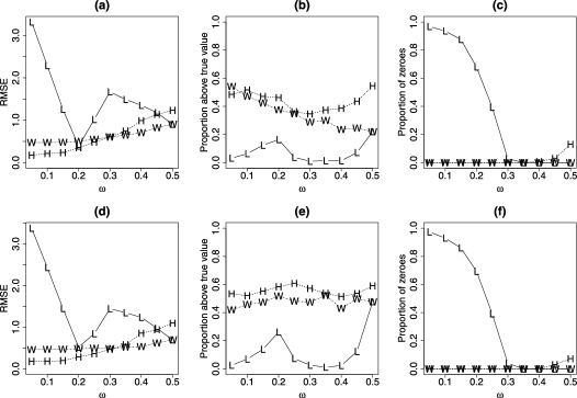
Figure 3: (a): RMSE of non-zero log probabilities, (b): proportion of estimates exceeding the true probability, and (c): proportion of zero probability estimates versus $\omega$ for the bivariate normal distribution with $\rho=0.5$; (d), (e), (f): as (a), (b), (c) but for the inverted bivariate extreme value distribution with logistic dependence structure and dependence parameter $\alpha=-\log 0.75/\log 2$. Plot characters ‘H’, ‘L’, ‘W’ refer to the methodology of Heffernan and Tawn [10], Ledford and Tawn [14] and the current authors, respectively.

Overall, the methodology, similarly to the theory, provides something of a compromise between that of Ledford and Tawn [14] and of Heffernan and Tawn [10]. One advantage of the new results is that one should rarely be in a position where a probability is estimated as identically zero, which we have argued can be a drawback to the existing nonparametric methodology.

For $\omega=0.5$, using the Hill estimator for $\eta$, the results from the methodology of Ledford and Tawn [14] and the current paper are the same, since we have $1/\eta=\kappa(1,1)=2\lambda(1/2)$. Away from the diagonal however, the results of the Ledford and Tawn [14] model, which rely on estimating empirical probabilities through (1) with $v+\log n+A=(1.5\log 5000,\infty)\times(\{\omega/(1-\omega)\}1.5\log 5000,\infty)$, deteriorate greatly. This reflects the fact that the theory underlying the methodology is designed for joint tails, where both variables grow at the same rate. For angles $\omega<0.3$ in this example, we observe a rapid rise in the number of zero probability estimates, see Figure 3(c) and (f). In any real application, this could be a serious problem as only a single sample is available. The problem of having an empirical probability of zero in a joint survivor set could in theory be partially solved by noting that for any angle $\omega_{1}<\omega_{2}$ the latter set is nested in the former, and one could sum the zero and non-zero component. This however provides rather poor estimates, and so we do not adopt this strategy for the reported results.

The methodology of Heffernan and Tawn [10] shows steady improvements in RMSE as the angle $\omega$ decreases, and the joint survivor set moves closer to being a marginal probability. This is owing to the form of the limit theory involved. Recall equations (20) and (4.2). Let $\hat{a},\hat{b}$ denote the estimates of the normalizing functions, and define the $i$th component of a residual vector by $Z_{i}:=\{X_{E,i}-\hat{b}(Y_{E,i})\}/\hat{a}(Y_{E,i})$. Making $j=1,\ldots,r$ new draws $Y_{E,j}^{*}$ from the exponential distribution, conditionally upon being larger than $(1-\omega)u_{n}$, and $r$ draws from the empirical distribution function of the residuals, the required probability can be estimated by

$$\mbox{{P}}\bigl{\{}Y_{E}>(1-\omega)u_{n}\bigr{\}}\frac{1}{r}\sum_{j=1}^{r}I\bigl{\{}\hat{a}\bigl{(}Y_{E,j}^{*}\bigr{)}Z_{j}+\hat{b}\bigl{(}Y_{E,j}^{*}\bigr{)}>\omega u_{n}|Y_{E,j}^{*}>(1-\omega)u_{n}\bigr{\}}.$$ (30)

When $(1-\omega)u_{n}$ is large but $\omega u_{n}$ small, it is the marginal probability $\mbox{{P}}\{Y_{E}>(1-\omega)u_{n}\}$ which is important for accurate estimation. This ensures increasing precision of estimation near the axes. The reliance of the estimator (30) upon an empirical residual vector highlights how zero probability estimates are a potential problem, since only certain trajectories of the new variable $\hat{a}(Y_{E,j}^{*})Z_{j}+\hat{b}(Y_{E,j}^{*})$ are possible. This problem occurs only rarely here, though some evidence of it for angles $\omega$ near 0.5 is apparent from Figure 3(c) and (f), but the issue intensifies as the sample size decreases or dimension increases. For an additional discussion, see Peng and Qi [17].

The simple estimator we propose provides consistently reasonable estimates across the whole range of angles $\omega$. In further simulation results, not reported, we found that the RMSE can be improved close to the axes ($\omega$ near 0 or 1), to a level similar to the Heffernan and Tawn [10] methodology, by replacing the random exponential sample with rank-transformed data; that is, the $i$th largest value $X_{E,(i)}$ is replaced by $-\log\{i/(n+1)\}$.

Figure 2, along with Figure 3(b) and (e) illustrate the effect that the non-constant slowly varying function of the normal distribution has in comparison to the unit slowly varying function of the inverted bivariate extreme value distribution. Figure 3(b) shows a small bias on the diagonal $\omega=0.5$ under the proposed estimation method, which gradually decreases as the angle moves towards the axes. The true conditional excess probability is

$$\frac{L^{*}(nt;\omega)}{L^{*}(n;\omega)}t^{-\lambda(\omega)}=t^{-[\lambda(\omega)-\{\log L^{*}(nt;\omega)-\log L^{*}(n;\omega)\}/\log t]}.$$

For the normal distribution, estimation of $\lambda$ will therefore exhibit some bias which is more pronounced in the range of $\omega$ such that $L_{1}(n;\omega,1-\omega)$, as identified in equation (1), is non-constant; this is observed in Figure 2(a). This bias can be seen to decay at rate $\mathrm{O}(1/\log n)$, and thus will persist for nearly all practical sample sizes. However, this fact ensures that the theoretical bias in $\lambda$ estimation is not as severe from a practical perspective, since it remains largely unchanged over the range for which we are likely to be interested in extrapolation. Figures 2(b) and 3(e) show that the estimation of $\lambda$ for the inverted bivariate extreme value distribution is unbiased for all angles, as should be expected given that $L\equiv 1$.

6 Discussion

The theory presented has provided a characterization of tail probability decay rates for a wide variety of multivariate distributions. The results apply both in the case of asymptotically independent and dependent random vectors. However, richer theoretical representations are gained in the case of asymptotic independence in two dimensions, or an analogous notion of weak joint tail dependence in three or more dimensions, as defined in Section 2.4. The theory developed strongly mirrors the existing representation for asymptotically dependent distributions, however it is exploited in the characterization of tail probability decay rates rather than the characterization of limit distributions. In particular, we find that the homogeneous function $\kappa$ and angular dependence function $\lambda$ play roles under weak joint tail dependence which are very similar to the roles of the exponent function $V$ and Pickands’ dependence function $A$ of the classical theory for asymptotic dependence. Multivariate extreme value theory is most often approached from a perspective of multivariate regular variation. We have demonstrated how generalizing multivariate regular variation of $(X_{P},Y_{P})$ to that of $(X_{P}^{1/\omega},Y_{P}^{1/(1-\omega)})$ provides a representation which encodes dependence information under both asymptotic dependence and asymptotic independence.

From a statistical perspective, we have demonstrated that a simple methodological procedure can provide very reasonable estimates of bivariate joint survivor probabilities across the whole of the positive quadrant. In addition, we have argued that in providing a theoretical and methodological compromise between the approaches of Ledford and Tawn [14] and Heffernan and Tawn [10], we can overcome some of the methodological difficulties which can surface in either of these two cases. In statistical applications, it is difficult to be certain whether data are asymptotically independent or dependent, and to apply the proposed methodology we need make no distinction.

The theory upon which we have focused is particularly suited to the extrapolation of joint survivor sets, where only a single ray $\omega$ is implicated. Estimation of probabilities of more general sets can be achieved in theory through exploitation of limit (18). However, rates of convergence to such limits may be slow. There is clearly also a choice of limit distributions in this case, and investigations into the most suitable trajectory of extrapolation for a given set of interest, in terms of optimizing the rate of convergence to the limit, remains an open avenue for further research.

References

- [1] {bbook}[mr] \bauthor\bsnmBeirlant, \bfnmJan\binitsJ., \bauthor\bsnmGoegebeur, \bfnmYuri\binitsY., \bauthor\bsnmTeugels, \bfnmJozef\binitsJ. &\bauthor\bsnmSegers, \bfnmJohan\binitsJ. (\byear2004). \btitleStatistics of Extremes: Theory and Applications. \bseriesWiley Series in Probability and Statistics. \blocationChichester: \bpublisherWiley. \biddoi=10.1002/0470012382, mr=2108013 \bptokimsref \endbibitem
- [2] {barticle}[mr] \bauthor\bsnmColes, \bfnmStuart G.\binitsS.G. &\bauthor\bsnmTawn, \bfnmJonathan A.\binitsJ.A. (\byear1991). \btitleModelling extreme multivariate events. \bjournalJ. R. Stat. Soc. Ser. B Stat. Methodol. \bvolume53 \bpages377–392. \bidissn=0035-9246, mr=1108334 \bptokimsref \endbibitem
- [3] {barticle}[mr] \bauthor\bparticlede \bsnmHaan, \bfnmLaurens\binitsL. &\bauthor\bparticlede \bsnmRonde, \bfnmJohn\binitsJ. (\byear1998). \btitleSea and wind: Multivariate extremes at work. \bjournalExtremes \bvolume1 \bpages7–45. \biddoi=10.1023/A:1009909800311, issn=1386-1999, mr=1652944 \bptokimsref \endbibitem
- [4] {barticle}[mr] \bauthor\bparticlede \bsnmHaan, \bfnmLaurens\binitsL. &\bauthor\bsnmResnick, \bfnmSidney\binitsS. (\byear1998). \btitleOn asymptotic normality of the Hill estimator. \bjournalComm. Statist. Stochastic Models \bvolume14 \bpages849–866. \biddoi=10.1080/15326349808807504, issn=0882-0287, mr=1631534 \bptokimsref \endbibitem
- [5] {barticle}[mr] \bauthor\bsnmHaeusler, \bfnmE.\binitsE. &\bauthor\bsnmTeugels, \bfnmJ. L.\binitsJ.L. (\byear1985). \btitleOn asymptotic normality of Hill’s estimator for the exponent of regular variation. \bjournalAnn. Statist. \bvolume13 \bpages743–756. \biddoi=10.1214/aos/1176349551, issn=0090-5364, mr=0790569 \bptokimsref \endbibitem
- [6] {barticle}[mr] \bauthor\bsnmHall, \bfnmPeter\binitsP. &\bauthor\bsnmTajvidi, \bfnmNader\binitsN. (\byear2000). \btitleDistribution and dependence-function estimation for bivariate extreme-value distributions. \bjournalBernoulli \bvolume6 \bpages835–844. \biddoi=10.2307/3318758, issn=1350-7265, mr=1791904 \bptokimsref \endbibitem
- [7] {barticle}[mr] \bauthor\bsnmHashorva, \bfnmEnkelejd\binitsE. &\bauthor\bsnmHüsler, \bfnmJürg\binitsJ. (\byear2003). \btitleOn multivariate Gaussian tails. \bjournalAnn. Inst. Statist. Math. \bvolume55 \bpages507–522. \biddoi=10.1007/BF02517804, issn=0020-3157, mr=2007795 \bptokimsref \endbibitem
- [8] {barticle}[mr] \bauthor\bsnmHeffernan, \bfnmJanet\binitsJ. &\bauthor\bsnmResnick, \bfnmSidney\binitsS. (\byear2005). \btitleHidden regular variation and the rank transform. \bjournalAdv. in Appl. Probab. \bvolume37 \bpages393–414. \biddoi=10.1239/aap/1118858631, issn=0001-8678, mr=2144559 \bptokimsref \endbibitem
- [9] {barticle}[mr] \bauthor\bsnmHeffernan, \bfnmJanet E.\binitsJ.E. &\bauthor\bsnmResnick, \bfnmSidney I.\binitsS.I. (\byear2007). \btitleLimit laws for random vectors with an extreme component. \bjournalAnn. Appl. Probab. \bvolume17 \bpages537–571. \biddoi=10.1214/105051606000000835, issn=1050-5164, mr=2308335 \bptokimsref \endbibitem
- [10] {barticle}[mr] \bauthor\bsnmHeffernan, \bfnmJanet E.\binitsJ.E. &\bauthor\bsnmTawn, \bfnmJonathan A.\binitsJ.A. (\byear2004). \btitleA conditional approach for multivariate extreme values (with discussion). \bjournalJ. R. Stat. Soc. Ser. B Stat. Methodol. \bvolume66 \bpages497–546. \biddoi=10.1111/j.1467-9868.2004.02050.x, issn=1369-7412, mr=2088289 \bptokimsref \endbibitem
- [11] {barticle}[mr] \bauthor\bsnmHill, \bfnmBruce M.\binitsB.M. (\byear1975). \btitleA simple general approach to inference about the tail of a distribution. \bjournalAnn. Statist. \bvolume3 \bpages1163–1174. \bidissn=0090-5364, mr=0378204 \bptokimsref \endbibitem
- [12] {bbook}[mr] \bauthor\bsnmJoe, \bfnmHarry\binitsH. (\byear1997). \btitleMultivariate Models and Dependence Concepts. \bseriesMonographs on Statistics and Applied Probability \bvolume73. \blocationLondon: \bpublisherChapman & Hall. \bidmr=1462613 \bptokimsref \endbibitem
- [13] {barticle}[mr] \bauthor\bsnmLedford, \bfnmAnthony W.\binitsA.W. &\bauthor\bsnmTawn, \bfnmJonathan A.\binitsJ.A. (\byear1996). \btitleStatistics for near independence in multivariate extreme values. \bjournalBiometrika \bvolume83 \bpages169–187. \biddoi=10.1093/biomet/83.1.169, issn=0006-3444, mr=1399163 \bptokimsref \endbibitem
- [14] {barticle}[mr] \bauthor\bsnmLedford, \bfnmAnthony W.\binitsA.W. &\bauthor\bsnmTawn, \bfnmJonathan A.\binitsJ.A. (\byear1997). \btitleModelling dependence within joint tail regions. \bjournalJ. R. Stat. Soc. Ser. B Stat. Methodol. \bvolume59 \bpages475–499. \biddoi=10.1111/1467-9868.00080, issn=0035-9246, mr=1440592 \bptokimsref \endbibitem
- [15] {barticle}[mr] \bauthor\bsnmMaulik, \bfnmKrishanu\binitsK. &\bauthor\bsnmResnick, \bfnmSidney\binitsS. (\byear2004). \btitleCharacterizations and examples of hidden regular variation. \bjournalExtremes \bvolume7 \bpages31–67. \biddoi=10.1007/s10687-004-4728-4, issn=1386-1999, mr=2201191 \bptokimsref \endbibitem
- [16] {bbook}[mr] \bauthor\bsnmNiculescu, \bfnmConstantin P.\binitsC.P. &\bauthor\bsnmPersson, \bfnmLars-Erik\binitsL.E. (\byear2006). \btitleConvex Functions and Their Applications: A Contemporary Approach. \bseriesCMS Books in Mathematics/Ouvrages de Mathématiques de la SMC \bvolume23. \blocationNew York: \bpublisherSpringer. \bidmr=2178902 \bptokimsref \endbibitem
- [17] {barticle}[author] \bauthor\bsnmPeng, \bfnmL.\binitsL. &\bauthor\bsnmQi, \bfnmY.\binitsY. (\byear2004). \btitleDiscussion of “A conditional approach for multivariate extreme values,” by J. E. Heffernan and J. A. Tawn. \bjournalJ. R. Stat. Soc. Ser. B Stat. Methodol. \bvolume66 \bpages541–542. \bptokimsref \endbibitem
- [18] {binproceedings}[mr] \bauthor\bsnmPickands, \bfnmJames\binitsJ. (\byear1981). \btitleMultivariate extreme value distributions. In \bbooktitleBulletin of the International Statistical Institute: Proceedings of the 43rd Session (Buenos Aires) \bpages859–878. \blocationVoorburg, Netherlands: \bpublisherISI. \bidmr=820979 \bptokimsref \endbibitem
- [19] {barticle}[mr] \bauthor\bsnmRamos, \bfnmAlexandra\binitsA. &\bauthor\bsnmLedford, \bfnmAnthony\binitsA. (\byear2009). \btitleA new class of models for bivariate joint tails. \bjournalJ. R. Stat. Soc. Ser. B Stat. Methodol. \bvolume71 \bpages219–241. \biddoi=10.1111/j.1467-9868.2008.00684.x, issn=1369-7412, mr=2655531 \bptokimsref \endbibitem
- [20] {barticle}[mr] \bauthor\bsnmResnick, \bfnmSidney\binitsS. (\byear2002). \btitleHidden regular variation, second order regular variation and asymptotic independence. \bjournalExtremes \bvolume5 \bpages303–336. \biddoi=10.1023/A:1025148622954, issn=1386-1999, mr=2002121 \bptokimsref \endbibitem
- [21] {bbook}[mr] \bauthor\bsnmResnick, \bfnmSidney I.\binitsS.I. (\byear1987). \btitleExtreme Values, Regular Variation, and Point Processes. \bseriesApplied Probability. A Series of the Applied Probability Trust \bvolume4. \blocationNew York: \bpublisherSpringer. \bidmr=0900810 \bptokimsref \endbibitem
- [22] {bbook}[mr] \bauthor\bsnmResnick, \bfnmSidney I.\binitsS.I. (\byear2007). \btitleHeavy-Tail Phenomena: Probabilistic and Statistical Modeling. \bseriesSpringer Series in Operations Research and Financial Engineering. \blocationNew York: \bpublisherSpringer. \bidmr=2271424 \bptnotecheck year\bptokimsref \endbibitem
- [23] {barticle}[mr] \bauthor\bsnmRuben, \bfnmHarold\binitsH. (\byear1964). \btitleAn asymptotic expansion for the multivariate normal distribution and Mills’ ratio. \bjournalJ. Res. Nat. Bur. Standards Sect. B \bvolume68B \bpages3–11. \bidissn=0160-1741, mr=0165622 \bptokimsref \endbibitem
- [24] {barticle}[author] \bauthor\bsnmSavage, \bfnmI. R.\binitsI.R. (\byear1962). \btitleMills’ ratio for multivariate normal distributions. \bjournalJournal of Research of the National Bureau of Standards B \bvolume66B \bpages93–96. \bptokimsref \endbibitem
- [25] {barticle}[mr] \bauthor\bsnmTawn, \bfnmJonathan A.\binitsJ.A. (\byear1988). \btitleBivariate extreme value theory: Models and estimation. \bjournalBiometrika \bvolume75 \bpages397–415. \biddoi=10.1093/biomet/75.3.397, issn=0006-3444, mr=0967580 \bptokimsref \endbibitem
- [26] {bmisc}[author] \bauthor\bsnmWadsworth, \bfnmJ. L.\binitsJ.L. (\byear2012). \bhowpublishedModels for penultimate extreme values. Ph.D. thesis, Lancaster Univ. \bptokimsref \endbibitem