Catalog of narrow $\rm C~{}IV$ absorption lines in BOSS (I): for quasars with $\rm z_{em}\leq 2.4$

Abstract

We have assembled absorption systems by visually identifying $\rm C~{}IV\lambda\lambda 1548,1551$ absorption doublets in the quasar spectra of the Baryon Oscillation Spectroscopic Survey (BOSS) one by one. This paper is the first of the series work. In this paper, we concern quasars with relatively low redshifts and high signal-to-noise ratios for their spectra, and hence we limit our analysis on quasars with $z_{\rm em}\leq 2.4$ and on the doublets with $W_{r}\lambda 1548\geq 0.2$ Å.  Out of the more than 87,000 quasars in the Data Release 9, we limit our search to 10,121 quasars that have the appropriate redshifts and spectra with high enough signal-to-noise ratios to identify narrow C IV absorption lines. Among them, 5,442 quasars are detected to have at least one $\rm C~{}IV\lambda\lambda 1548,1551$ absorption doublet. We obtain a catalog containing 8,368 $\rm C~{}IV\lambda\lambda 1548,1551$ absorption systems, whose redshifts are within $z_{\rm abs}=1.4544$ — $2.2805$. In this catalog, about 33.7% absorbers have $0.2$ Å$\leq W_{r}\lambda 1548<0.5$ Å,  about 45.9% absorbers have $0.5$ Å$\leq W_{r}\lambda 1548<1.0$ Å,  about 19.2% absorbers have $1.0$ Å$\leq W_{r}\lambda 1548<2.0$ Å,  and about 1.2% absorbers have $W_{r}\lambda 1548\geq 2.0$ Å.

1. Introduction

Absorption lines are often observed in the quasar spectra, which are a powerful tool to probe the gas in the Universe from high redshifts to the present epoch (see Meiksin 2009 for a review). Quasar absorption lines provide an unique chance to study the gaseous phase (e.g., ionization states, kinematics, metallicities) of distant galaxies that otherwise might be invisable, which are independent of the luminosity of the background quasars. They are also important to understand the star formation and evolution of the ordinary galaxies (e.g., Prochter et al. 2006; Zibetti et al. 2007; Ménard et al. 2011; Chen 2013).

Narrow absorption lines (NALs), with the line width of a few hundred $\rm km~{}s^{-1}$, can be classified into three categories according to the relationship between the absorber and the corresponding quasar. They are intrinsic absorption lines, associated absorption lines and intervening absorption lines. The intrinsic absorption lines are often believed to be physically related with the quasar wind/outflow (e.g., Narayanan et al. 2004; Misawa et al. 2007; Hamann et al. 2011). The associated absorption lines with $z_{\rm abs}\approx z_{\rm em}$ probably arise from the gas in the quasar host galaxy or the galaxy cluster around the quasar (e.g., Weymann et al. 1979; Wild et al. 2008; Vanden Berk et al. 2008). The intervening absorption lines with $z_{\rm abs}\ll z_{\rm em}$ are due to the absorption of galaxies along the quasar sightlines located at cosmological distances from the corresponding quasars (e.g., Bahcall & Spitzer 1969; Bergeron 1986; López & Chen 2012). The criteria, determining whether the absorption lines are truly tied to the corresponding quasars, is ambiguous, because there are many factors that can disturb the observed absorption lines, such as the signal to noise ratio of the quasar spectra. To day the dividing line of the intervening absorption lines and the associated absorption lines are usually derived by statistics (e.g., Richards 2001; Wild et al. 2008). The absorption lines at velocity separations less than the value of $\rm\sim 0.02c-0.04c$, when compared to the quasar systems, are classified as associated absorption line group (Vanden Berk et al. 2008; Wild et al. 2008). However, that does not mean that narrow absorption lines with velocity separation larger than that value completely belong to intervening absorption lines. Narrow intrinsic absorption lines can be formed in the quasar outflows with velocity separations up to, and even exceeding $\rm 0.1c$ (e.g., Misawa et al. 2007; Tombesi et al. 2011; Chen et al. 2013a; Chen & Qin 2013).

$\rm C~{}IV\lambda\lambda 1548,1551$ resonant doublets are observable redward of the $\rm Ly\alpha 1216$ emission line, which can be detected over a redshift range of $z\approx 1.5$ — 5.5 in the optical spectra. These lines are strong transitions and have good profiles. They are valuable absorption lines to study the intergalactic medium (e.g., Songaila & Cowie 1996; Cowie & Songaila 1998; Songaila 2001; Schaye et al. 2003; Cooksey et al. 2010; DÓdorico et al. 2010; Simcoe et al. 2011).

Based on the Sloan Digital Sky Survey (SDSS, York et al. 2000), many previous works aimed at systematically searching for metal absorption lines have been done (e.g., Quider et al. 2011; Qin et al. 2013; Zhu & Ménard 2013; Cooksey et al. 2013). We are going to identify absorption doublets, such as $\rm C~{}IV\lambda\lambda 1548,1551$ and $\rm Mg~{}II\lambda\lambda 2796,2803$, in the quasar spectra of the Baryon Oscillation Spectroscopic Survey (BOSS), which is a part of the SDSS-III (Eisenstein et al. 2011). In this paper, our work is to identify the $\rm C~{}IV\lambda\lambda 1548,1551$ absorption doublet, which becomes the first in a series of papers on the absorption lines in the BOSS quasar spectra.

In section 2, we show how we construct our $\rm C~{}IV\lambda\lambda 1548,1551$ absorption sample and present the spectral analysis. The properties of the absorption lines are presented in section 3. Section 4 is the discussion, and section 5 is the summary.

2. Data analysis

BOSS is the main dark time legacy survey of the third stage of the SDSS (Pâris et al. 2012; Eisenstein et al. 2011), which is a five year programm. BOSS aims to get quasar spectra over $150,000$ with $z_{\rm em}>2.15$ using the same $\rm 2.5m$ telescope (Gunn et al. 2006; Ross et al. 2012) as the SDSS did. The spectra of BOSS span a wavelength range of 3600 Å— 10400 Å  at a resolution of $1300<R<3000$. The first data release of BOSS, SDSS Data Release Nine (SDSS DR9), contains $87,822$ quasars detected over an area of $3275~{}deg^{2}$ (Pâ aris et al. 2012).

In order to avoid the noisy region of the spectra, we exclude those data shortward of 3800 Å  at the observed frame. The pair of $\rm O~{}I\lambda 1302$ and $\rm S~{}II\lambda 1304$ has a wavelength separation similar to that of the $\rm C~{}IV\lambda\lambda 1548,1551$ doublet, and that may lead to misidentifications of the latter. To avoid confusions arising from the $\rm Ly\alpha$ forest, and $\rm O~{}I\lambda 1302$ and $\rm S~{}II\lambda 1304$ absorption lines, we constrain our analysis on the wavelength range longward of 1310 Å  at the rest frame. We also conservatively constrain the upper wavelength limit to $\rm 1548$Å$\rm\times(1+z_{em})\times\sqrt{(1-\beta)/(1+\beta)}$, where we adopt $\rm\beta=-1/30$ to search for intervening $\rm C~{}IV\lambda\lambda 1548,1551$ absorption doublets. This cut reduces the quasar sample to $70,336$ quasars with $z_{em}\gtrsim 1.54$.

The noise superposed on the spectra with low signal-to-noise ratios (SNR) often confuses the true absorptions. Here, we limit our analysis to sources with high enough signal-to-noise ratios in the surveyed spectral region. There is a median signal-to-noise ratio (median SNR) of the spectrum of each quasar, which can roughly reveal the level of the noise of the observation of the source. Illustrated in Fig. 1 is the distribution of the median SNR of these $70,336$ quasars. We find that the median value of this distribution is quite close to $4$ (see Fig. 1). We accordingly adopt this value to limit our analysis. That is, we select only quasars with $\rm median~{}SNR\geq 4$ in the surveyed spectral region.

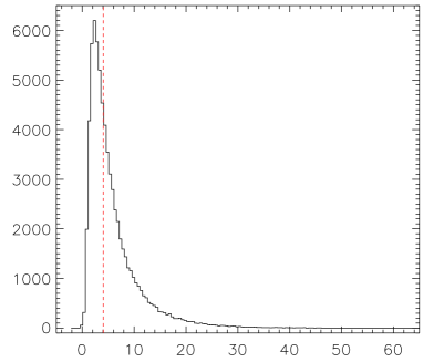
Figure 1.— Distribution of the median SNR of the 70,336 quasars, in the surveyed spectral region of $\rm C~{}IV\lambda\lambda 1548,1551$ absorption doublets. The red dash line denotes the median value of this distribution, which is located at 4.06.

As the first paper of the series of work, here we concern only quasars with $z_{\rm em}\leq 2.4$. Taking into account all the above limitations, we have 10,121 quasars with $1.54\lesssim z_{\rm em}\leq 2.4$ to identify $\rm C~{}IV\lambda\lambda 1548,1551$ absorption doublets. The upper cuts of the emission redshift and the median SNR are showed in Fig. 2. The distribution of emission redshifts of our final quasar sample is plotted in Fig. 4.

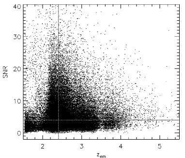
Figure 2.— Plot of the median SNR, in the surveyed spectral region of $\rm C~{}IV\lambda\lambda 1548,1551$ absorption doublets, versus the emission redshift of the $70,336$ quasars. The red lines are the limits of SNR and $z_{em}$ used to construct our quasar sample.

We derive a pseudo-continuum for each quasar of our sample by invoking a combination of cubic splines (for underlying continuum, see Willian et al. 1992 for details) and Gaussians (for emission and broad absorption features), which is utilized to normalize the spectral data (fluxes and flux uncertainties). These processes are iterated several times to improve the fittings of both the cubic spline and Gaussian (e.g., Nestor et al. 2005; Quider et al. 2011, Chen et al. 2013a,b). Shown in the left panels of Fig. 3 are several quasar spectra (with various values of the median SNR) together with their pseudo-continuum fitting curves. The pseudo-continuum normalized spectra are presented in the right panels of Fig. 3.

We search $\rm C~{}IV\lambda\lambda 1548,1551$ absorption candidates from the pseudo-continuum normalized spectra. As the first step of the searching (see also Chen et al. 2013a), the $2\sigma$ curve below the pseudo-continuum fitting is marked, and then those absorption figures located above this curve are ruled out.

In many cases, some very broad troughs appear in the blue wing of $\rm C~{}IV$ or/and $\rm Si~{}IV$ emission lines. The broad absorption line (BAL) is a confusing terminology. Based on the definition of balnicity index (BI, Weymann et al. 1991), absorption troughs with the width broader than $2000~{}\rm km~{}s^{-1}$ at depths $>10\%$ below the pseudo-continuum fitting curve can be classified as BALs. However, in terms of the absorption index (AI, Hall et al. 2002; Trump et al. 2006), some narrower absorption troughs ($>1000~{}\rm km~{}s^{-1}$) also belong to the BAL population. Knigge et al. (2008) found that the BAL fraction will be underestimated in terms of BI, and overestimated in terms of AI. They also found that both samples of BI and AI show bimodal distributions, which bring about a problem of the overlap of broad NALs and narrow BALs. We are going to analyze only narrow absorption doublets with a few hundreds $km~{}s^{-1}$, therefore, as the second step, we conservatively disregard those absorption figures with widths broader than $2000~{}\rm km~{}s^{-1}$ and at depths $>10\%$ below the pseudo-continuum fitting curve in our program autonomically.

In the third step, each absorption trough is fitted by a Gaussian component, and the absorption figures with the full width at half maximum (FWHM) greater than $800~{}\rm km~{}s^{-1}$ are ruled out. And then, we search the candidates of $\rm C~{}IV\lambda\lambda 1548,1551$ absorption doublets from the residual absorption figures.

In the fourth step, we measure the equivalent widths ($W_{r}$) of these candidate absorption lines at the rest-frame from the Gaussian fittings, and estimate their uncertainties by

$$(1+z)\sigma_{w}=\frac{\sqrt{\sum_{i}P^{2}(\lambda_{i}-\lambda_{0})\sigma^{2}_{f_{i}}}}{\sum_{i}P^{2}(\lambda_{i}-\lambda_{0})}\Delta\lambda,$$ (1)

where $P(\lambda_{i}-\lambda_{0})$ is the line profile centered at $\lambda_{0}$, $\lambda_{i}$ is the wavelength, and $\sigma_{f_{i}}$ is the normalized flux uncertainty as a function of pixel (Nestor et al. 2005; Chen et al. 2013b; Chen & Qin 2013). The sum is performed over an integer number of pixels that covers at least $\pm 3$ characteristic Gaussian widths. We adopt the method provided by Qin et al. (2013) to evaluate the signal-to-noise ratio of the absorption line for the candidates as well. $\rm 1\sigma$ noise is calculated by:

$$\sigma_{N}=\sqrt{\frac{\sum\limits_{i=1}^{M}[\frac{F^{i}_{noise}}{F^{i}_{cont}}]^{2}}{M}},$$ (2)

where $\rm F_{noise}$ is the flux uncertainty, $\rm F_{cont}$ is the flux of the psuedo-continuum fit, and $i$ represents the pixel in the wavelength range of 1548Å$\rm\times(1+z_{abs})-5$Å$\rm<\lambda_{obs}<1551$Å$\rm\times(1+z_{abs})+5$Å. The signal-to-noise ratio of the absorption line is determined by:

$$SNR^{\lambda}=\frac{1-S_{abs}}{\sigma_{N}},$$ (3)

where $\rm S_{abs}$ is the smallest value of the normalized spectral flux within an absorption trough. Finally, we select only the absorption lines with $W_{r}>0.2$ Å  and $SNR^{\lambda}\geq 2.0$ for both $\lambda 1548$ and $\lambda 1551$ lines. In this way, we get 8368 potential intervening $\rm C~{}IV\lambda\lambda 1548,1551$ absorption doublets. These absorption doublets are presented in Table 1.

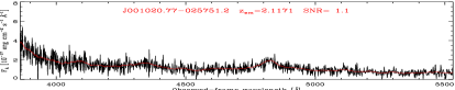
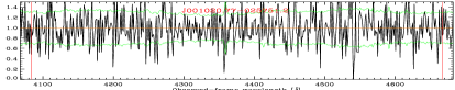
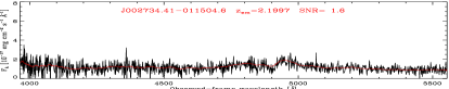
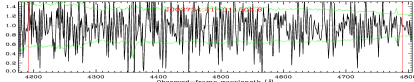
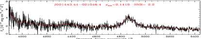
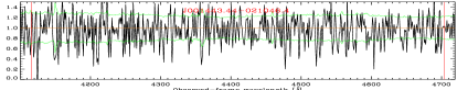
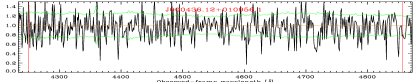
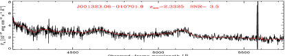
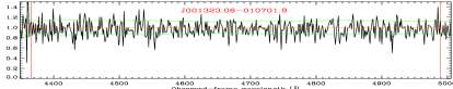
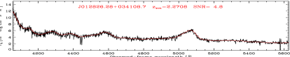
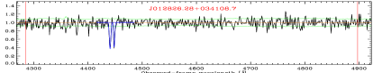
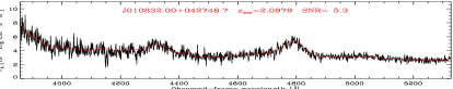
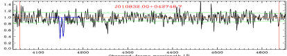
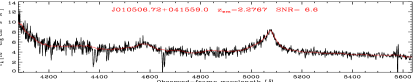
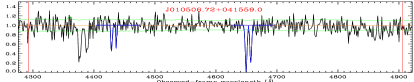
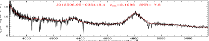
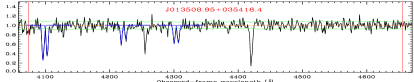
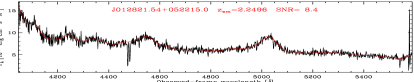
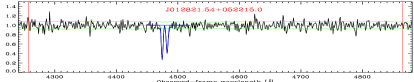
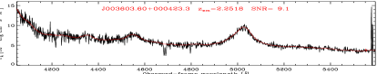
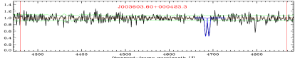
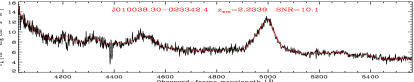
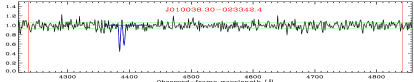
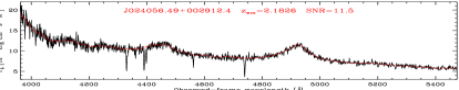
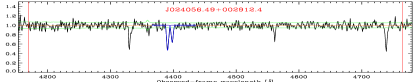
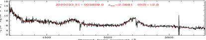
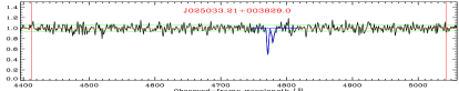
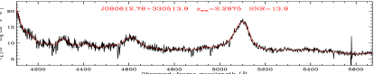
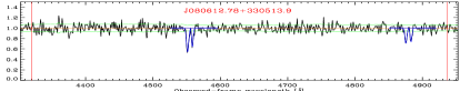
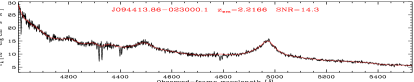
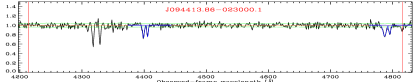
Figure 3.— The quasar spectra with various values of the median signal-to-noise ratio (SNR) in the searched spectral region of $\rm C~{}IV\lambda\lambda 1548,1551$ absorption doublets. The red curves in the left panels represent the pseudo-continuum fitting curves. The green lines in the right panels represent the $1\sigma$ flux uncertainty levels that have been normalized by the pseudo-continuum. The blue solid lines are the Gaussian fitting curves of the doublets. The red vertical lines in the right panels represent the lower and upper limitations respectively, which are used to cut the spectral region to search for $\rm C~{}IV\lambda\lambda 1548,1551$ absorption doublets. We do not search the $\rm C~{}IV\lambda\lambda 1548,1551$ absorption doublet in the spectra with SNR less than 4 (e.g., the first five spectra).

Table 1Catalog of $\rm C~{}IV\lambda\lambda 1548,1551$ absorption systems

SDSS NAME	PLATEID	MJD	FIBERID	$z_{\rm em}$	$z_{\rm abs}$	$\rm W_{r}\lambda 1548$	$N_{\sigma\lambda 1548}$	$\rm W_{r}\lambda 1551$	$N_{\sigma\lambda 1551}$	$SNR^{\lambda 1548}$	$SNR^{\lambda 1551}$	$\beta$
000027.01+030715.5	4296	55499	0630	2.3533	1.9833	0.22	4.40	0.22	4.40	3.9	4.4	0.11639
000027.01+030715.5	4296	55499	0630	2.3533	2.1303	0.91	22.75	0.69	17.25	20.3	18.3	0.06871
000050.59+010959.1	4216	55477	0746	2.3678	1.8971	0.46	7.67	0.47	5.88	7.1	5.3	0.14942
000050.59+010959.1	4216	55477	0746	2.3678	1.9184	0.99	14.14	0.86	14.33	13.6	13.0	0.14225
000120.27+030731.9	4277	55506	0098	2.1082	1.8898	0.38	7.60	0.25	6.25	6.6	5.3	0.07273
000133.39+023657.1	4277	55506	0090	1.6556	1.4773	0.71	2.84	0.67	4.47	2.7	4.2	0.06939
000146.95+001428.9	4216	55477	0860	2.1567	1.9256	0.39	3.90	0.38	6.33	3.8	5.6	0.07588
000202.33-002648.4	4216	55477	0154	2.1761	1.9382	0.59	3.47	0.35	3.18	3.3	2.9	0.07770
000207.61+032801.5	4296	55499	0748	2.2195	1.7502	1.25	6.58	0.86	6.14	6.2	5.9	0.15626
000223.32+010101.2	4216	55477	0876	2.2931	2.1549	0.32	2.91	0.45	3.21	2.6	3.1	0.04285

Note—$N_{\sigma}=\frac{W_{r}}{\sigma_{W}}$ represents the significant level of the detection. $\beta=\frac{v}{c}=\frac{(1+z_{em})^{2}-(1+z_{abs})^{2}}{(1+z_{em})^{2}+(1+z_{abs})^{2}}$. The table is available in its entirety in the machine-readable form in the online journal.

3. Statistical properties of the absorbers

In this work, we collect 10,121 quasars to identify $\rm C~{}IV\lambda\lambda 1548,1551$ absorption doublets, whose emission redshifts are plotted in Fig. 4. Of the 10,121 quasar spectra, 5,442 are found to have at least one detected $\rm C~{}IV\lambda\lambda 1548,1551$ absorption doublet. Emission redshifts of these 5,442 quasars are also plotted in Fig. 4. We identify 8,368 $\rm C~{}IV\lambda\lambda 1548,1551$ absorption doublets from these quasars. These absorption redshifts are also showed in the Fig. 4.

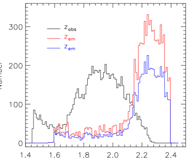
Figure 4.— Distributions of redshifts. The red line represents the emission redshift of 10,121 quasars that are used to search for $\rm C~{}IV\lambda\lambda 1548,1551$ absorption doublets. The blue line stands for the emission redshift of the 5442 quasars for which at least one $\rm C~{}IV\lambda\lambda 1548,1551$ absorption doublet is detected. The black line describes the absorption redshift of all the detected $\rm C~{}IV\lambda\lambda 1548,1551$ absorption doublets.

The total redshift path covered by this catalog can be computed via

$$Z(SNR^{\lambda 1548})=\sum_{i=1}^{N_{spec}}\int_{z_{i}^{min}}^{z_{i}^{max}}g_{i}(SNR^{\lambda 1548},z)dz,$$ (4)

where $\rm g_{i}(SNR^{\lambda 1548},z)=1$ if $\rm SNR^{lim}~{}\leq SNR^{\lambda 1548}$, otherwise $\rm g_{i}(SNR^{\lambda 1548},z)=0$; $\rm z_{i}^{min}$ and $\rm z_{i}^{max}$ are the redshifts corresponding to the minimum and maximum wavelengths of survey for quasar $i$, respectively (see also Qin et al. 2013). The derived redshift path is shown in Fig. 5 as a function of the signal-to-noise ratio.

Figure 5.— Redshift path covered by our catalog ($z_{\rm em}\leq 2.4$), shown as a function of $\rm SNR^{\lambda 1548}$.

Distributions of $W_{r}$ of the two lines of the $\rm C~{}IV\lambda\lambda 1548,1551$ absorption doublet of our catalog are plotted in Fig. 6. These distributions have smooth tails out to $W_{r}\approx 3.0$ Å,  with the largest values of $W_{r}\lambda 1548=3.19$ Å  and $W_{r}\lambda 1551=2.88$ Å,  respectively. The median values of the $W_{r}$ are: 0.62 Å  for the $\lambda 1548$ absorption lines, and 0.49 Å  for the $\lambda 1551$ absorption lines. In this catalog, about 33.7% (2823/8368) absorbers have $0.2$ Å$\leq W_{r}\lambda 1548<0.5$ Å,  about 45.9% (3842/8368) absorbers have $0.5$ Å$\leq W_{r}\lambda 1548<1.0$ Å,  about 19.2% (1603/8368) absorbers have $1.0$ Å$\leq W_{r}\lambda 1548<2.0$ Å,  and about 1.2% (100/8368) absorbers have $W_{r}\lambda 1548\geq 2.0$ Å.

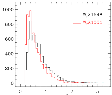
Figure 6.— Distributions of the rest-frame equivalent width of the $\rm C~{}IV$ absorption line. The black line is for the $\rm\lambda 1548$ absorption, and the red line is for the $\rm\lambda 1551$ absorption.

In Fig. 7 we plot the distribution of the $W_{r}$ ratio of the two lines ($W_{r}\lambda 1548/W_{r}\lambda 1551$). We invoke a Gaussian function to fit this distribution, which yields a center value of 1.18 and $\rm FWHM=0.80$. The maximum and minimum values of the $W_{r}$ ratio are 4.5 and 0.2, respectively. The $W_{r}$ ratio can reflects the saturated degree (Strömgren 1948). The $W_{r}$ ratio of the $\rm C~{}IV\lambda\lambda 1548,1551$ doublet can be changed from completely saturated absorption, $\rm DR=1.0$, to completely unsaturated absorption, $\rm DR=2.0$ (e.g., Sargent et al. 1988; Steidel 1990). The boundaries of the completely saturated absorption ($\rm DR=1.0$) and completely unsaturated absorption ($\rm DR=2.0$) are marked in Fig. 7. Most of the absorbers of this catalog satisfy $1.0\leq W_{r}\lambda 1548/W_{r}\lambda 1551\leq 2.0$, occupying nearly 72.9% (6007/8638) of the total. About 22.0% (1839/8638) absorbers have $W_{r}\lambda 1548/W_{r}\lambda 1551<1.0$, and about 6.2% (522/8638) absorbers have $W_{r}\lambda 1548/W_{r}\lambda 1551>2.0$. We guess that the $\rm C~{}IV\lambda\lambda 1548,1551$ absorption systems that lie outside the theoretical limits of the $W_{r}$ ratio ($W_{r}\lambda 1548/W_{r}\lambda 1551<1.0$ or $W_{r}\lambda 1548/W_{r}\lambda 1551>2.0$) might mainly originate from the line blending.

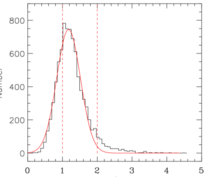
Figure 7.— Distribution of the ratio of the rest-frame equivalent widthes of the $\rm C~{}IV$ doublet. The red curve is the fitting Gaussian with $\rm center=1.18~{}and~{}FWHM=0.80$. The red dash lines are the theoretical limits for completely saturated ($\rm W_{r}\lambda 1548/W_{r}\lambda 1551=1.0$) and unsaturated ($\rm W_{r}\lambda 1548/W_{r}\lambda 1551=2.0$) absorptions, respectively.

4. Discussion

In order to estimate the false positives/negatives of the $\rm C~{}IV$ absorption system, we wish to look at the frequency of the detected $\rm C~{}IV$ absorption systems ($f_{NALs}$) as a function of signal-to-noise ratio, which can be computed via

$$f_{NALs}=\lim_{\bigtriangleup SNR\rightarrow 0}\frac{\bigtriangleup N_{abs}}{\bigtriangleup N_{sdp}}$$ (5)

where $\bigtriangleup N_{abs}$ and $\bigtriangleup N_{sdp}$ are the count of the detected $\rm C~{}IV$ absorption systems and the count of the spectral data points in signal-to-noise ratio bin $\bigtriangleup SNR$, respectively. The resulting $f_{NALs}$, as a function of the signal-to-noise ratio, is displayed in Fig. 8. It exhibits a platform in the range of $SNR^{\lambda 1548}\gtrsim 4$, suggesting that the detection of $C~{}IV$ absorption systems would likely be complete when the signal-to-noise ratio is larger than 4.

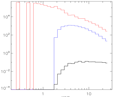
Figure 8.— Plot of the detection frequency as a function of the signal-to-noise ratio. The upper (red) line represents the count of the spectral data point, the middle (blue) line represents the count of the detected $\rm C~{}IV$ absorption system, and the bottom (black) line stands for the frequency of NALs detected in this work, calculated by equation (5).

The incompleteness of the detection of $C~{}IV$ absorption systems is obvious within the range of $SNR^{\lambda 1548}\lesssim 4$. As suggested by Fig. 8, we find that, within the range of $SNR^{\lambda 1548}\lesssim 4$, when the signal-to-noise ratio tends to be smaller, more $C~{}IV$ absorption systems would tend to be missed by our analysis. To roughly estimate the significance of the incompleteness, we compute the missing rate ($f_{MR}$) of the detection of $C~{}IV$ absorption systems in several bins of the signal-to-noise ratio via

$$f_{MR}=\frac{\overline{f_{NALs}}-f_{NALs}}{\overline{f_{NALs}}},$$ (6)

where $\overline{f_{NALs}}$ is the average frequency of NALs in the range of $SNR^{\lambda 1548}>4$, and $f_{NALs}$ is the frequency of NALs in the corresponding signal-to-noise ratio bin. The results are presented in Table 2.

Table 2The missing rate of absorption systems with $SNR^{\lambda 1548}\leq 4$

SNR bin	[2.0,2.5]	[2.5,3.0]	[3.0,3.5]	[3.5,4.0]
$f_{MR}$	0.91	0.67	0.62	0.20

To refine the quasar sample to search the $\rm C~{}IV\lambda\lambda 1548,1551$ absorption system, we perform our analysis under the condition that the spectra examined must have a median signal-to-noise ratio greater than or equal to $4$. It is possible that some $\rm C~{}IV\lambda\lambda 1548,1551$ absorption doublets, which satisfy our criteria of selecting absorption lines, may be imprinted in the spectra with the median signal-to-noise ratio being less than $4$, and they will be missed.

To have a look at these possibly missed doublets, we randomly select $100$ quasars from those located in the left lower region of Fig. 2 (below the horizontal red line and on the left hand side of the vertical red line), to detect $\rm C~{}IV\lambda\lambda 1548,1551$ absorption doublets with the same criteria described in section 2. These quasars are listed in Table 3. $15$ $\rm C~{}IV\lambda\lambda 1548,1551$ absorption doublets are detected from these quasar spectra, which are presented in Table 4. For this randomly selected quasar sample, the redshift path computed using Equation (4) and the frequency of NALs calculated by Equation (5) are displayed in Figs. 9 and 10, respectively.

Table 3Sources of the randomly selected quasar sample

SDSS NAME	PLATEID	MJD	FIBERID	$z_{\rm em}$	SNR
000525.86+030813.5	4296	55499	0908	2.1802	3.4
00063.085+031327.1	4296	55499	0962	2.3788	3.9
002059.05+030633.3	4300	55528	0716	2.1935	3.4
004616.50+011343.0	3589	55186	0864	2.1632	1.5
005623.89+021253.2	4308	55565	0740	2.2631	2.1
010618.39+101247.8	4551	55569	0598	2.2872	1.3
011927.05+000008.0	4227	55481	0036	2.3571	1.7
013752.51+102410.6	4548	55565	0802	2.1453	2.7

Note—SNR is the median signal-to-noise ratio of the quasar in the surveyed spectral region. The table is available in its entirety in the machine-readable form in the online journal.

Table 4The $\rm C~{}IV\lambda\lambda 1548,1551$ absorption systems of the randomly selected quasar sample

SDSS NAME	PLATEID	MJD	FIBERIN	$z_{\rm em}$	$z_{\rm abs}$	$\rm W_{r}\lambda 1548$	$N_{\sigma\lambda 1548}$	$\rm W_{r}\lambda 1551$	$N_{\sigma\lambda 1551}$	$SNR^{\lambda 1548}$	$SNR^{\lambda 1551}$	$\beta$
075343.86+182204.9	4490	55629	0734	2.1708	1.9708	0.38	2.53	0.56	2.55	2.3	2.4	0.06506
114931.76+360338.8	4653	55622	0042	2.2658	1.7910	0.79	2.39	1.21	3.67	2.2	3.4	0.15582
014848.55+145729.2	4658	55592	0948	2.1370	1.8690	0.31	2.38	0.44	2.44	2.2	2.3	0.08907
152155.41+310942.3	4719	55736	0322	2.1108	1.8249	0.88	5.18	0.39	2.79	4.4	2.7	0.09611
080345.70+422136.2	3683	55178	0178	2.0877	1.6675	0.61	3.81	0.71	3.23	3.5	3.0	0.14525
155717.07+163309.6	3922	55333	0594	2.3355	2.1045	0.81	3.12	0.71	2.84	2.9	2.7	0.07165
081937.46+302718.3	4447	55542	0070	2.2037	2.0069	0.58	2.76	0.65	2.83	2.7	2.7	0.06331
074256.10+481730.0	3675	55183	0520	2.2775	1.9637	1.14	3.93	0.99	3.41	3.6	3.2	0.10030
150553.69+304300.5	3876	55245	0264	2.2329	1.7556	1.02	2.83	0.74	3.08	2.7	3.0	0.15840
134259.55+340404.9	3856	55269	0612	2.2972	2.1021	0.77	2.75	0.43	2.39	2.6	2.3	0.06092
024842.21-000302.1	4241	55450	0265	2.0587	1.8580	0.59	3.11	0.46	2.88	3.0	2.7	0.06776
150914.76+230044.0	3962	55660	0610	2.1652	1.9392	1.04	2.89	0.79	2.39	2.7	2.3	0.07394
150539.79+062612.3	4856	55712	0230	2.3698	2.0359	0.88	3.03	1.19	3.31	2.9	3.1	0.10397
104647.31+382734.8	4634	55626	0932	2.2235	1.9783	1.20	2.86	0.76	2.38	2.7	2.2	0.07895
094705.52+434013.8	4569	55631	0764	2.1984	1.9500	1.14	4.75	1.60	3.48	4.1	3.3	0.08067

Note—See Table 1 for the meanings of each column.

Figure 9.— Redshift path covered by the randomly selected quasar sample, shown as a function of $\rm SNR^{\lambda 1548}$.

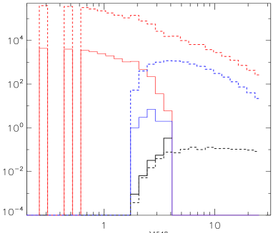
Figure 10.— Plot of the detection frequency as a function of the signal-to-noise ratio for the randomly selected quasar sample. See Fig. 8 for the meanings of each solid line. The dash lines are the solid lines shown in Fig. 8 with the same colors.

The spectral signal-to-noise ratio is important to detect narrow absorption lines. It is very difficult to distinguish the true NALs from the noise in the spectra with lower signal-to-noise ratio, since the fluctuations of the noise frequently confuse or cover the real narrow absorption lines. As stated above, only 15 $\rm C~{}IV$ absorption systems are detected in the spectra of the 100 randomly selected quasars. In other words, only 0.15 $\rm C~{}IV$ absorption system can be detected in per quasar spectrum with the median signal-to-noise ratio being as low as less than 4. However, we detect 8,368 $\rm C~{}IV$ absorption systems in the spectra of the 10,121 quasars with their median signal-to-noise ratios being greater than 4. The value of 8368/10121 is several times larger than that of 15/100, which manifests that many real absorption lines cannot be identified in the spectra with lower signal-to-noise ratios.

5. Summary

As the first effort in our series work on identifying absorption lines in quasar spectra of BOSS, we search quasars with $z_{\rm em}\leq 2.4$ and identify potential intervening $\rm C~{}IV\lambda\lambda 1548,1551$ absorption doublets with $W_{r}\lambda 1548\geq 0.2$ Å . Our sample contains 10,121 quasars, from which we identify 8,368 $\rm C~{}IV\lambda\lambda 1548,1551$ absorption systems which covers the absorption redshift range of $z_{\rm abs}=1.4544$ — $2.2805$. Of 10,121 quasars, 5,442 are detected to have at least one $\rm C~{}IV\lambda\lambda 1548,1551$ absorption doublet. We find that about 33.7% absorbers have $0.2$ Å$\leq W_{r}\lambda 1548<0.5$ Å,  about 45.9% absorbers have $0.5$ Å$\leq W_{r}\lambda 1548<1.0$ Å,  about 19.2% absorbers have $1.0$ Å$\leq W_{r}\lambda 1548<2.0$ Å,  and about 1.2% absorbers have $W_{r}\lambda 1548\geq 2.0$ Å. Most of the $\rm C~{}IV\lambda\lambda 1548,1551$ absorption doublets (72.9%) lie within the theoretical limits of the completely saturated and unsaturated absorptions ($1.0\leq W_{r}\lambda 1548/W_{r}\lambda 1551\leq 2.0$).

References

- (1) Bahcall, J. N., & Spitzer, L. Jr. 1969, ApJ, 156, L63
- (2) Bergeron, J. 1986, A&A, 155, L8
- (3) Cowie, L. L., & Songaila, A. 1998, Nature, 394, 44
- (4) Cooksey, K. L., Thom, C., Prochaska, J. X., & Chen, H. 2010, ApJ, 708, 868
- (5) Cooksey, K. L., Kao, M. M., Simcoe, R. A., O’Meara, J. M. & Prochaska, J. X. 2013, ApJ,763, 37
- (6) Chen, Z. F. 2013, RAA, 13, 641
- (7) Chen, Z. F., Li, M. S., Huang, W. R., Pan, C. J., & Li, Y. B. 2013a, MNRAS, 434, 3275
- (8) Chen, Z. F., Qin, Y. P., Gu, M. F. 2013b, ApJ, 770, 59
- (9) Chen, Z. F., & Qin, Y. P. 2013, ApJ, 776, 1
- (10) DÓdorico, V., Calura, F., Cristiani, S., & Viel, M. 2010, MNRAS, 401, 2715
- (11) Eisenstein, D. J., et al., 2011, AJ, 142, 72
- (12) Gunn, J. E., et al., 2006, AJ, 131, 2332
- (13) Hall, P ., Anderson, S., Strauss, M., York, D., Richards, G., & Fan, X. e. A. 2002, ApJS, 141, 267
- (14) Hamann F., Kanekar N., Prochaska J. K., et al. 2011, MNRAS, 410, 1957
- (15) Knigge, G., Scaringi, S., Goad, M. R., & Cottis, C. E. 2008, MNRAS, 386, 1426
- (16) López, G., & Chen, H. W. 2012, MNRAS, 419, 3553
- (17) Misawa T., Charlton J. C., Eracleous M., et al. 2007, ApJS, 171, 1
- (18) Meiksin, A. A. 2009, Rev. Mod. Phys., 81, 1405
- (19) Ménard, B., Wild, V., Nestor, D., et al. 2011, MNRAS, 417, 801
- (20) Narayanan D., Hamann F., Barlow T., et al. 2004, ApJ, 601, 715
- (21) Nestor, D. B., Turnshek, D. A., Rao, S. M. 2005, ApJ, 628, 637
- (22) Prochter, G. E., Prochaska, J. X., & Burles, S. M. 2006, ApJ, 639, 766
- (23) Pâris, I. et al., 2012, A&A, 548, 66
- (24) Quider, A. M., Nestor, D. B., Turnshek, D. A., et al.. 2011, AJ, 141, 137
- (25) Qin, Y. P., Chen, Z. F., Lü, L. Z., et al. 2013, PASJ, 65, 8
- (26) Richards, G. T. 2001, ApJS, 133, 53
- (27) Ross, N. P., Myers, A. D., Sheldon, E. S., et al. 2012, ApJS, 199, 3
- (28) Strömgren, B. 1948, ApJ, 108, 242
- (29) Sargent, W. L. W., Boksenberg, A., & Steidel, C. C. 1988, ApJS, 68, 539
- (30) Steidel, C. C. 1990, ApJS, 72, 1
- (31) Songaila, A., & Cowie, L. L. 1996, AJ, 112, 335
- (32) Songaila, A. 2001, ApJ, 561, L153
- (33) Schaye, J., Aguirre, A., Kim, T. S., et al. 2003, ApJ, 596, 768
- (34) Simcoe, R. A., Cooksey, K. L., Matejek, M., et al. 2011, ApJ, 743, 21
- (35) Trump, J., et al. 2006, ApJS, 165, 1
- (36) Tombesi, F., Cappi, M., Reeves, J. N., et al. 2011, ApJ, 742, 44
- (37) Vanden Berk, D. E., Khare, P., York, D. G., et al. 2008, ApJ, 679, 239
- (38) Weymann, R. J., Williams, R. E., Peterson, B.M., & Turnshek, D. A. 1979, ApJ, 234, 33
- (39) Weymann, R., Morris, S., Foltz, C., & Hewett, P . 1991, ApJ, 373, 23
- (40) Willian, H. P., Teukolsky, S. A., Willian, T. V., Flannery, B. P., 1992, Numerical Recipes in Fortran: The Art of Scientific Computing. Cambridge Univ. Press, Cambridge, p. 107
- (41) Wild, V., Kauffmann, G., White, S., et al. 2008, MNRAS, 388, 227
- (42) York, D. G., Adelman, J., Anderson, J. E., Jr., et al. 2000, AJ, 120, 1579
- (43) Zibetti, S., Ménard, B., Nestor, D. B., et al. 2007, ApJ, 658, 161
- (44) Zhu, G. T., & Ménard, B. 2013, ApJ, 770, 130