On Spatial Transition Probabilities as Continuity Measures in Categorical Fields

Abstract

Models of spatial transition probabilities, or equivalently, transiogram models have been recently proposed as spatial continuity measures in categorical fields. In this paper, properties of transiogram models are examined analytically, and three important findings are reported. Firstly, connections between the behaviors of auto-transiogram models near the origin and the spatial distribution of the corresponding category are carefully investigated. Secondly, it is demonstrated that for the indicators of excursion sets of Gaussian random fields, most of the commonly used basic mathematical forms of covariogram models are not eligible for transiograms in most cases; an exception is the exponential distance-decay function and models that are constructed from it. Finally, a kernel regression method is proposed for efficient, non-parametric joint modeling of auto- and cross-transiograms, which is particularly useful for situations where the number of categories is large.

Keywords: categorical data, transition probability, geostatistics, spatial continuity

1 Introduction

Categorical spatial data, such as land use and land cover data in geography and environmental science, rock (lithology) types in earth science and socio-economic survey data in social sciences, etc., are all-important information sources across a wide spectrum of scientific fields. As with continuous spatial data, complex spatial patterns (spatial correlation) exist in such geo-referenced categorical data in accordance with Tobler’s first law of geography (Tobler, 1970). A successful investigation of the statistical characteristics in these patterns will benefit many of the above mentioned scientific fields, particularly with respect to spatial data classification or clustering, spatial uncertainty modeling and spatial scale effects. In remote sensing imagery classification, for example, spatial pattern information implied in thematic classes (e.g., forest area is more likely adjacent to grassland than desert area) can be fully integrated with conventional classifiers to enhance the classification performance (Tso and Mather, 2001).

One of the most fundamental concepts in spatial analysis is the choice of spatial continuity measures usually quantifying similarity in attribute values or class labels. In conventional geostatistics, indicator kriging (IK) (Solow, 1986) and indicator coKriging (ICK) (Deutsch and Journel, 1998) are the most frequently used methods for estimating the posterior (conditional) probability of class occurrence at any unsampled location conditioned on the available observed data. Both IK and ICK rely on two-point spatial continuity measures, indicator (cross)covariance or (cross)variogram models, for characterizing spatial association in categorical spatial data. Although covariances and variograms are suitable for continuous fields, particularly Gaussian random fields, the discrete characteristics of categorical data, along with their sharp boundaries and complex spatial patterns, render the interpretation of such covariances and variograms less intuitive. This, in turn, hinders the applications of the kriging family of methods for deriving probabilities of class occurrence in categorical fields.

Recently, promising alternatives to the indicator (cross-)variogram, namely, spatial transition probabilities (Carle and Fogg, 1996), or equivalently, transiograms (Li, 2006), have been proposed as alternative spatial continuity measures in categorical fields. The concept of transition probability is not new; but it has only recently been proposed as a continuity measure in categorical fields. Compared to indicator covariances and variogram models, transiograms are more interpretable in categorical fields, and easier to integrate with ancillary information (Carle and Fogg, 1996). Based on this concept, Carle and Fogg (1996) reformulated IK and ICK as systems of spatial transition probabilities according to their analytical connections with indicator covariograms. More recently, Li (2007b) employed a single Markov Chain moving randomly within a stationary random field (Markov Chain Random Field) for conditional simulation or interpolation of categorical spatial data. Class occurrence probabilities derived by such methods usually satisfy the fundamental probability constraints naturally compared to methods based on variations of IK.

As an extension of transition probabilities in a spatial setting, transiograms naturally inherit basic properties of two-point conditional probabilities, such as asymmetry, non-negativity and unit-sum (Carle and Fogg, 1996, 1997). The relationships between the parameters of transiogram models and the information on class proportion, mean length, and class juxtaposition have been investigated by Carle and Fogg (1996), and this information actually provides an interpretation of the behavior of transiogram models and eventually offers a guideline for the construction of such models by incorporating expert knowledge of the spatial distribution of the categories under study. Along these lines, one potential contribution of this paper is to investigate the connections between the behavior of auto-transiogram models near the origin and the spatial distribution of the associated category.

As with variograms, not every function of distance can serve as a valid transiogram. Several basic mathematical models of variograms, such as circular, spherical, exponential, Gaussian, and cosine-Gaussian, have been proposed for transiogram modeling (Li and Zhang, 2006). No discussion, however, has yet been made on whether these valid variogram functions can be eligible for transiograms under certain circumstances. In this paper, the validity of transiogram models in the stationary indicator random fields, particularly the excursion sets of Gaussian Random Fields (GRFs), is discussed and it is found that in most cases, only the exponential form and several of its variants are eligible for transiogram modeling.

On another front, even if valid transiograms are assumed to be available, or in cases where the assumption of stationary indicator random fields does not apply, e.g., in a Markov Chain Random Field (MCRF) (Li, 2007b), transiogram model fitting from empirical values can become tedious as the number of classes increases, since there are $K^{2}$ auto- and cross-transiogram curves to be jointly modeled for a set of $K$ classes. In practice, one often finds that basic parametric transiogram models (usually defined by a set of parameters including range, sill, anisotropy and etc.) cannot capture the irregular fluctuations at small scales (e.g., hole effect) often found in empirical transiograms. Incorporating this information in transiogram models could dramatically increase the number of (unknown) parameters to be estimated (Li et al., 2011), and renders the quantitative fitting of such models infeasible. To address these computing and modeling issues, this paper proposes a kernel regression-based non-parametric fitting procedure for efficient and consistent transiogram modeling.

The remainder of this paper is organized as follows: the behavior of auto-transiograms near the origin is examined in Section 3 after briefly reviewing the concepts of transiograms in Section 2. Section 4 is devoted to investigating the validity of basic transiogram models in the excursion sets of GRFs, and the kernel regression based non-parametric transiogram model fitting method is presented in Section 5. Finally, section 6 concludes the paper and provides some discussion.

2 Basic concepts of spatial transition probabilities

Consider a $d$-dimensional geographical region $\Omega$ which is partitioned into $N$ disjoint subregions with a categorical random variable (RV) $C(\boldsymbol{x})$ ($\boldsymbol{x}\in R^{d}$) which can take one out of $K$ mutually exclusive and collectively exhaustive class labels $c(\boldsymbol{x})\in\{1,\ldots,K\}$ at any arbitrary location with coordinate vector $\boldsymbol{x}$. Alternatively, one can also define an indicator variable $I_{k}(\boldsymbol{x})$ to represent $C(\boldsymbol{x})$, where $I_{k}(\boldsymbol{x})=1$ if $C(\boldsymbol{x})=k$ and $I_{k}(\boldsymbol{x})=0$ otherwise.

Given two locations $\boldsymbol{x}$ and $\boldsymbol{x}^{\prime}$ in $\Omega$, and the associated class labels denoted as $k$ and $k^{\prime}$, the transiogram $\pi_{k^{\prime}|k}(\boldsymbol{x}^{\prime},\boldsymbol{x})$ is typically a parametric model of transition probabilities as a function of the lag vector $\boldsymbol{h}=\boldsymbol{x}^{\prime}-\boldsymbol{x}$. In words, $\pi_{k^{\prime}|k}(\boldsymbol{x}^{\prime},\boldsymbol{x})$ is the probability of, starting from a source location $\boldsymbol{x}$ with class label $k$, arriving at a destination location $\boldsymbol{x}^{\prime}$ with class label $k^{\prime}$. Note that since the dimension of $\Omega$ is greater than $1$, there are theoretically infinite paths to reach a destination location $\boldsymbol{x}^{\prime}$ from a source location $\boldsymbol{x}$. This equifinality issue hinders the application of the original definition of 1D transition probability and the rich Markov chain theory based on it, such as the celebrated Chapman-Kolmogrov equation, to high dimensional spaces. To eliminate ambiguity, the definition of spatial transition probabilities is restricted to the path defined by the vector $\boldsymbol{h}=\boldsymbol{x}^{\prime}-\boldsymbol{x}$. Specifically, spatial transition probabilities could be defined as:

$$\pi_{k^{\prime}|k}(\boldsymbol{h}) = P\{C(\boldsymbol{x}^{\prime})=k^{\prime}|C(\boldsymbol{x})=k\}$$ (1)

$$= P\{I_{k^{\prime}}(\boldsymbol{x}^{\prime})=1|I_{k}(\boldsymbol{x})=1\}$$

$$= \frac{P\{I_{k^{\prime}}(\boldsymbol{x}^{\prime})=1\;and\;I_{k}(\boldsymbol{x})=1\}}{P\{I_{k}(\boldsymbol{x})=1\}}$$

Second-order or intrinsic stationarity (Chilès and Delfiner, 1999) is implicitly assumed in this definition, since the value of $\pi_{k^{\prime}|k}(\boldsymbol{h})$ depends only on the lag $\boldsymbol{h}$ and not on the location $\boldsymbol{x}$ or $\boldsymbol{x}^{\prime}$. More specifically, $\pi_{k|k}(\boldsymbol{h})$ denotes the auto-transiogram for class $k$ (when $k=k^{\prime}$), a measure of spatial auto-correlation of class $k$, and $\pi_{k^{\prime}|k}(\boldsymbol{h})$ denotes the cross-transiogram from class $k$ to class $k^{\prime}$ (when $k\neq k^{\prime}$), a measure of spatial cross-correlation between class $k$ and class $k^{\prime}$. Conventionally, class $k$ and class $k^{\prime}$ in $\pi_{k^{\prime}|k}(\boldsymbol{h})$ are called tail class and head class respectively.

Under the assumption of second-order stationarity, sample transiograms can be obtained by direct computation (exhaustive sampling, no parametric model involved) from sample data on a regular grid whose node spacing coincides with the scale of analysis. Thus for a given $\boldsymbol{h}$, we have:

$$\hat{\pi}_{k^{\prime}|k}(\boldsymbol{h})\simeq\frac{1}{\pi_{k}}E\{I_{k}(\boldsymbol{x})I_{k^{\prime}}(\boldsymbol{x}+\boldsymbol{h})\}\simeq\frac{1}{\pi_{k}N(\boldsymbol{h})}\sum_{n=1}^{N(\boldsymbol{h})}[i_{k}(\boldsymbol{x})i_{k^{\prime}}(\boldsymbol{x}+\boldsymbol{h})]$$ (2)

where $N(\boldsymbol{h})$ denotes the number of location pairs separated by vector $\boldsymbol{h}$ and $\pi_{k}$ indicates the proportion of class $k$. Figure.1 provides an area-class map with three categories, and for a certain lag distance $\boldsymbol{h}$, the associated transiograms ($3\times 3$) values are computed by exhaustively enumerating the pairs of nodes separated by a template vector $\boldsymbol{h}$ in the whole sample map.

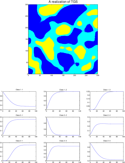
Figure 1: A sample area-class map (top) with three classes and its associated transiograms curves (bottom) are computed by exhaustive sampling (scanning). All two-point dependence information of the area-class map is encapsulated in these ($3\times 3$) empirical transiogram curves.

If a (latent) probabilistic distribution is assumed underpinning the (observable) categorical field, e.g., a truncated multivariate Gaussian field, all auto- and cross-transiograms can be computed exactly according to the threshold values associated with each class and the analytical form of the latent distribution (Chilès and Delfiner, 1999).

The basic models of variograms as well as the classical geostatistical concepts of range, sill, hole effect, and anisotropy, have been discussed in the context of transiograms (Li, 2006). Given a lag vector $\boldsymbol{h}$, transiogram values (spatial transition probabilities) have the following basic properties:

• asymmetry

  $$\pi_{k^{\prime}|k}(\boldsymbol{h})\neq\pi_{k^{\prime}|k}(-\boldsymbol{h})$$ (3)

• non-negativity

  $$\pi_{k^{\prime}|k}(\boldsymbol{h})\geq 0,\forall k,k^{\prime}$$ (4)

• unit-sum

  $$\sum_{k^{\prime}=1}^{K}\pi_{k^{\prime}|k}(\boldsymbol{h})=1$$ (5)

• value at zero distance

  $$\pi_{k^{\prime}|k}(0)=\left\{\begin{array}[]{cc}1&\mbox{if $k=k^{\prime}$}\\ 0&\mbox{if $k\neq k^{\prime}$}\end{array}\right.$$ (6)

With the basic concepts and properties of the transiogram models reviewed in this section, the remainder of this paper will investigate the additional important properties of these models including the properties near the origin, validity of the transiogram models as well as the fitting procedures of these models.

3 Behaviors of Transiogram Models Near the Origin

As in covariograms, the shape (e.g., regularity) of transiograms reflects the spatial continuity and interaction of categories. In Figure.1, for example, the cross-transiogram curves between class $1$ (represented as $blue$ in Figure.1) and class $3$ (represented as $cyan$ in Figure.1) stay at $0$ for a certain distance before they begin to increase gradually. This transiogram behavior is because class $1$ is never adjacent to class $3$ in the reference map of Figure.1, and transiogram values should increase after the minimum distance between pixels of class $1$ and class $3$. This connection between transiogram curves and the shape of objects, particularly the first derivative of an auto-transiogram curve at the origin and the shape of objects of the category associated with that auto-transiogram, is examined in detail in this section.

We start with two particular properties of the indicator representation of categorical spatial variables:

$$P\{I_{k}(\boldsymbol{x})=1\}=E\{I_{k}(\boldsymbol{x})\}$$ (7)

and

$$P\{I_{k}(\boldsymbol{x})=1\;and\;I_{k^{\prime}}(\boldsymbol{x}+\boldsymbol{h})=1\}=E\{I_{k}(\boldsymbol{x})I_{k^{\prime}}(\boldsymbol{x}+\boldsymbol{h})\}$$ (8)

where $E\{I_{k}(\boldsymbol{x})I_{k^{\prime}}(\boldsymbol{x}+\boldsymbol{h})\}$ is known as the non-centered indicator cross-covariance or probabilistic version of geometric covariogram (Lantuejoul, 2002).

Suppose there is a circular region $A$ with category $k$ shifted by $\boldsymbol{h}$ to region $A_{h}$ as illustrated in Figure.2. In this case, the area of intersection $A\bigcap A_{h}$ (blue domain) represents $E\{I_{k}(\boldsymbol{x})I_{k}(\boldsymbol{x}+\boldsymbol{h})\}$, and the area of $A$ (blue domain and red domain) represents $P\{I_{k}(\boldsymbol{x})=1\}$ if the area of the whole region is assumed to be $one$. Thus according to the definition of the transiogram (Equation.1), $\pi_{k|k}(h)$ can be seen as the area of the blue domain divided by the area of the whole circle or the proportion of the blue domain in the white or red domain.

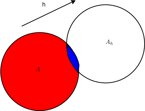
Figure 2: An illustration of non-center auto-transiogram

If the class proportions $E\{I_{k}(\boldsymbol{x})\}$ are assumed to be constant, one arrives to the analytical links between the transiogram and the indicator (cross-)covariogram and indicator (cross-)variogram by applying the properties of indicators (Equation.7 and Equation.8) to the definition of the (cross-)covariogram (Equation.9) and (cross-)variogram (Equation.10) respectively (Carle and Fogg, 1996):

$$\sigma_{kk^{\prime}}(\boldsymbol{h})=\pi_{k}[\pi_{k^{\prime}|k}(\boldsymbol{h})-\pi_{k^{\prime}}]$$ (9)

$$\gamma_{kk^{\prime}}(\boldsymbol{h})=\pi_{k}\{\pi_{k^{\prime}|k}(\boldsymbol{0})-[\pi_{k^{\prime}|k}(\boldsymbol{h})+\pi_{k^{\prime}|k}(-\boldsymbol{h})]/2\}$$ (10)

where $\sigma_{kk^{\prime}}(\boldsymbol{h})$ represents indicator (cross-)covariogram and $\gamma_{kk^{\prime}}(\boldsymbol{h})$ represents indicator (cross-)variogram and $\pi_{k^{\prime}|k}(-\boldsymbol{h})$ represents the transition probability in the opposite direction of $\boldsymbol{h}$. Particularly if we let $k=k^{\prime}$ and $\pi_{k|k}(0)=1$, we have a simple linear connection between the auto-transiogram and the indicator auto-variogram:

$$\pi_{k|k}(\boldsymbol{h})=1-\frac{\gamma_{kk}(\boldsymbol{h})}{\pi_{k}}$$ (11)

Because of the linear connection between the transiograms and the indicator (cross-)variogram/covariogram (Equation.9 and Equation.11), transiograms share the properties of indicator (cross-)variogram/covariograms. As Figure.1 illustrates, auto-transiograms (diagrams on the diagonal in Figure.1) start from $1$ at $\boldsymbol{h}=0$ and gradually decrease to the $sill$ value at $\boldsymbol{h}$ equals $range$, i.e., $\lim_{\boldsymbol{h}\rightarrow\infty}\pi_{k|k}(\boldsymbol{h})=\pi_{k}$. Cross-transiograms (diagrams off the diagonal in Figure.1) start from $0$ at $\boldsymbol{h}=0$ and gradually increase to the $sill$ value at $\boldsymbol{h}$ equals $range$, i.e., $\lim_{\boldsymbol{h}\rightarrow\infty}\pi_{k^{\prime}|k}(\boldsymbol{h})=\pi_{k^{\prime}}$.

The compactness of a geographic shape is an important property of a polygon in GIS/zoning and landscape metrics. One of the simplest compactness measures or indices of a shape is the ratio of its perimeter to its area (perimeter-to-area ratio) $\Psi$ (Smith et al., 2007). It is well known in the literature that the first derivative of the variogram at the origin is related to the derivative or gradient of the surface it represents (Stein, 1999; Chilès and Delfiner, 1999). Carle and Fogg (1996) have shown that in a 1D continuous-space Markov chain, the first derivative of the auto-transiogram at the origin, $\pi^{\prime}_{k|k}(\boldsymbol{0};\phi)$, termed transition rate, is related to the mean length or mean thickness of the objects of category $k$ in direction $\phi$. The empirical transition rate is usually calculated by the total length of category $k$ in direction $\phi$ divided by the number of embedded occurrences of $k$. In this paper, the relationship between the auto-transiogram for a certain class label and the perimeter-to-area ratio of shapes with such a class label in a 2D geographical space is given via the following proposition.

Proposition 3.1.

Under a stationary proportions assumption, the perimeter-to-area ratio $\Psi_{k}$ of the objects of category $k$ in a 2D random sets with $unit$ area can be obtained by integrating the derivative $\pi_{k|k}(0)$ in the direction $\phi$ at the origin over all possible directions:

$$\Psi_{k}=-\frac{1}{2}\int_{0}^{2\pi}\pi^{\prime}_{k|k}(\boldsymbol{0};\phi)d\phi$$ (12)

Proof 3.2.

In a 2D space, the perimeter $l_{k}$ of objects of category $k$ can be obtained by the application of Minkowski’s formula (Matheron, 1971; Lantuejoul, 2002):

$$l_{k}=-\frac{1}{2}\int_{0}^{2\pi}K^{\prime}_{\phi}(0)d\phi$$

where $K(\cdot)$ is the probabilistic version of geometric covariogram for category $k$ (Lantuejoul, 2002). Replacing the covariogram with the transiogram according to Equation.9, we have:

$$l_{k}=-\frac{\pi_{k}}{2}\int_{0}^{2\pi}\pi^{\prime}_{k|k}(0;\phi)d\phi$$

Under the stationary proportions assumption, $\pi_{k}$ is proportional to the area of objects of category $k$, and without loss of generality, one lets the total area equal $one$ and the area of objects of category $k$ is thus $\pi_{k}$. Equation.12 is obtained per the definition of the perimeter-to-area ratio.

For the isotropic case, $\Psi_{k}$ can then be simply written as:

$$\Psi_{k}=-\pi\times\pi^{\prime}_{k|k}(\boldsymbol{0})$$ (13)

If $\pi^{\prime}_{k|k}(\boldsymbol{0})=\infty$ in particular, it is anticipated that the boundaries of category $k$ demonstrate fractal properties. A degenerate case is when $\pi_{k|k}(\boldsymbol{h})$ is parabolic with $\pi^{\prime}_{k|k}(\boldsymbol{0})=0$.

It is worth noting that, in general, $\Psi_{k}$ is scale dependent and it is a particular average shape descriptor (of union) of objects of category $k$ instead of a single object; in other words, $\Psi_{k}$ corresponds to the mean perimeter-to-area ratio in landscape metrics (McGarigal and Marks, 1995). The conclusion of the Proposition.12 is for the closed objects. If the union object is open, the $boundary$ of the studied area will be taken into account. This note applies to both convex and concave shapes.

Proposition.12 can be verified by the circular region (the radius of this circle $R$ is assumed to be $0.25$) in a map with unit area (Figure.2). The perimeter-to-area ratio $\Psi_{A}=\frac{2}{R}=8$ and the auto-transiogram for category $k$ can be written as (the area of blue domain divided by the area of the circle):

$$\pi_{k|k}(\boldsymbol{h})=\frac{2}{\pi}\{\arccos(|\frac{\boldsymbol{h}}{2R}|)-|\frac{\boldsymbol{h}}{2R}|\sqrt{1-|\frac{\boldsymbol{h}}{2R}|^{2}}\}\mbox{ if }|\boldsymbol{h}|\leq R$$

Taking the first derivative of Equation.3 with respect to $\boldsymbol{h}$ and letting $\boldsymbol{h}=0$, one gets $\pi^{\prime}_{k|k}(0)=-\frac{2}{\pi R}=-\frac{8}{\pi}$ and Equation.13 is obviously satisfied.

Proposition.12 can further be illustrated in Figure.3. The $red$ curve in Figure.3 (a) represents the empirical auto-transiogram of class $3$ (represented as $yellow$) in the sample map Figure.3 (b), and $green$ curve represents that of the sample map Figure.3 (c). The areas of these two sample maps are exactly the same and the proportions of class $3$ ($yellow$ regions) are both about $0.40$. By comparing Figure.3 (b) and (c), one can easily check that the average perimeter of $yellow$ regions in (c) is much larger than that of (b). Thus according to the proposition.12, the auto-transiogram of class $3$ (the $red$ curve) in Figure.3 (b) should have a larger first derivative (slope) at the origin than that (the $green$ curve) of (c), which is evident by the two curves in Figure.3 (a).

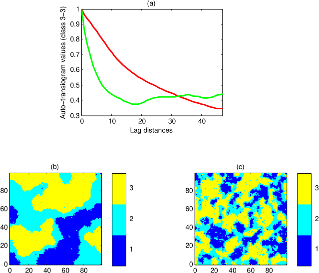
Figure 3: An illustration of connections between the first derivative of auto-transiograms at the origin and the shape of objects. (a) Empirical auto-transiograms of class $3$ in sample area-class maps (b) and (c) (b) a sample area-class map with three classes, and the empirical auto-transiogram of class $3$ (represented as $yellow$) is the $red$ curve in (a) (c) a sample area-class map with three classes, and the empirical auto-transiogram of class $3$ (represented as $yellow$) is the $green$ curve in (a).

In this section, the analytical connection between the auto-transiogram of a certain category, particularly its first derivative at the origin, and the shape metrics of the objects with this category in a categorical field is carefully investigated. It provides a quantitative interpretation of the behaviors of transiogram models. More importantly, together with other properties of transiograms (Carle and Fogg, 1997; Li, 2006), it provides analytical instructions for incorporating domain experts knowledge in transiogram-based applications.

4 Valid Transiogram Models

As in Kriging systems, one often needs to fit empirical transiogram values to certain parametric transiogram models in the transiogram-based methods (Carle and Fogg, 1996; Li, 2007b). Several theoretical models of variograms, such as triangular, circular, spherical, exponential and Gaussian, have been proposed as parametric models of transiograms (Li, 2006, 2007a) without checking their validity under certain circumstances. In this section, this validity is investigated in the stationary indicator random fields, particularly for indicators of excursion sets of GRFs, which is commonly used in geostatistics and spatial uncertainty modeling.

Let ${\bf Z}=\{Z(\boldsymbol{x})\}$ be a stationary GRF with a correlogram $\rho(\boldsymbol{h})$. Oftentimes, the indicators at location $\boldsymbol{x}$ $i_{k}(\boldsymbol{x})$ can be obtained by truncating $Z(\boldsymbol{x})$ by a specification of a cut-off value $z_{k}$, i.e.,

$$I_{k}(\boldsymbol{x})=\left\{\begin{array}[]{rl}1&\mbox{if $Z(\boldsymbol{x})\geq z_{k}$}\\ 0&\mbox{if otherwise}\end{array}\right.$$ (14)

It is of interest to determine whether the commonly-used triangular, circular, spherical, exponential and Gaussian variograms can be used to model the auto-transiogram of $I_{k}(\boldsymbol{x})$.

The triangular inequality for three random variables $Z(\boldsymbol{x})$, $Z(\boldsymbol{x}+\boldsymbol{h})$ and $Z(\boldsymbol{x}+\boldsymbol{h}+\boldsymbol{h}^{\prime})$ in a stationary random field is written as:

$$|Z(\boldsymbol{x}+\boldsymbol{h}+\boldsymbol{h}^{\prime})-Z(\boldsymbol{x})|\leq|Z(\boldsymbol{x}+\boldsymbol{h}+\boldsymbol{h}^{\prime})-Z(\boldsymbol{x}+\boldsymbol{h})|+|Z(\boldsymbol{x}+\boldsymbol{h})-Z(\boldsymbol{x})|$$

For indicator variables in particular, one has:

$$|I_{k}(\boldsymbol{x}+\boldsymbol{h}+\boldsymbol{h}^{\prime})-I_{k}(\boldsymbol{x})|\leq|I_{k}(\boldsymbol{x}+\boldsymbol{h}+\boldsymbol{h}^{\prime})-I_{k}(\boldsymbol{x}+\boldsymbol{h})|+|I_{k}(\boldsymbol{x}+\boldsymbol{h})-I_{k}(\boldsymbol{x})|$$

Moreover, $|I_{k}(\boldsymbol{x}+\boldsymbol{h})-I_{k}(\boldsymbol{x})|=|I_{k}(\boldsymbol{x}+\boldsymbol{h})-I_{k}(\boldsymbol{x})|^{2}$, which leads to a necessary condition for a valid indicator variogram:

$$\gamma_{kk}(\boldsymbol{h}+\boldsymbol{h}^{\prime})\leq\gamma_{kk}(\boldsymbol{h})+\gamma_{kk}(\boldsymbol{h}^{\prime})$$ (15)

A necessary condition for a valid auto-transiogram can thus be obtained by its analytical connections with an indicator auto-variogram (Equation.11):

$$\pi_{k|k}(\boldsymbol{h}+\boldsymbol{h}^{\prime})\geq\pi_{k|k}(\boldsymbol{h})+\pi_{k|k}(\boldsymbol{h}^{\prime})-1$$ (16)

According to the triangular inequality of auto-transiogram (Equation.16), the Gaussian form (Equation.19) cannot be a valid auto-transiogram, since if $\boldsymbol{h}=\boldsymbol{h}^{\prime}$, by the Equation.15 and Taylor expansion, we have $4|\boldsymbol{h}|^{2}\leq 2|\boldsymbol{h}|^{2}$ when $|\boldsymbol{h}|\rightarrow 0$, which is obviously a contradiction.

Matheron (1993) provided a more general necessary condition (containing the triangular inequality) for eligible indicator variograms $\gamma_{kk}(\boldsymbol{x},\boldsymbol{x}^{\prime})$: for any set of $m$ ($m\geq 2$) points $\boldsymbol{x}_{1},\ldots,\boldsymbol{x}_{m}$ with category $k$, and values $\epsilon_{i}\in\{-1;0;1\},i=1,\ldots,m$, such that $\sum_{i=1}^{m}\epsilon_{i}=1$, the associated variogram values $\gamma_{kk}(\boldsymbol{x}_{i},\boldsymbol{x}_{j})$ must satisfy:

$$\sum_{i=1}^{m}\sum_{j=1}^{m}\epsilon_{i}\epsilon_{j}\gamma_{kk}(\boldsymbol{x}_{i},\boldsymbol{x}_{j})\leq 0$$ (17)

Or equivalently, in terms of auto-transiogram values, one has :

$$\sum_{i=1}^{m}\sum_{j=1}^{m}\epsilon_{i}\epsilon_{j}(1-\pi_{k|k}(\boldsymbol{x}_{i},\boldsymbol{x}_{j}))\leq 0$$ (18)

It is still an open question whether the necessary condition is also sufficient for eligible indicator variograms of general random sets. Emery (2010) recently pursued this question further by suggesting that the properties of triangular, circular, and spherical variograms are rather restrictive in two or three dimensional indicator random fields, and proved that these three variograms are not valid indicator variograms for excursion sets of stationary GRFs. Due to the linear connection between indicator variograms and auto-transiograms, we can hence conclude that the Gaussian (Equation.19), triangular (Equation.20), spherical (Equation.21) and circular (Equation.22) models cannot be valid basic forms of auto-transiograms for indicators of excursion sets of stationary GRFs.

• Gaussian

  $$\pi_{k|k}(\boldsymbol{h})=1-(1-\pi_{k})\{1-\exp(-(\frac{|\boldsymbol{h}|}{a})^{2})\}$$ (19)

• Triangular

  $$\pi_{k|k}(\boldsymbol{h})=\left\{\begin{array}[]{cr}1-(1-\pi_{k})\frac{|\boldsymbol{h}|}{a}&\mbox{ if $\frac{|\boldsymbol{h}|}{a}\leq 1$}\\ \pi_{k}&\mbox{$o.w.$}\end{array}\right.$$ (20)

• Spherical

  $$\pi_{k|k}(\boldsymbol{h})=\left\{\begin{array}[]{cr}1-(1-\pi_{k})\{1.5\frac{|\boldsymbol{h}|}{a}-0.5(\frac{|\boldsymbol{h}|}{a})^{3}\}&\mbox{ if $\frac{|\boldsymbol{h}|}{a}\leq 1$}\\ \pi_{k}&\mbox{$o.w.$}\end{array}\right.$$ (21)

• Circular

  $$\pi_{k|k}(\boldsymbol{h})=\left\{\begin{array}[]{cr}1-(1-\pi_{k})\{1-\frac{2}{\pi}[\arccos(\frac{|\boldsymbol{h}|}{a})-\sqrt{1-(\frac{|\boldsymbol{h}|}{a})^{2}}]\}&\mbox{ if $\frac{|\boldsymbol{h}|}{a}\leq 1$}\\ \pi_{k}&\mbox{$o.w.$}\end{array}\right.$$ (22)

where $a$ represents the range parameter of the model.

To illustrate this conclusion, particularly for spherical cases, we assume that a spherical form (Equation.21) with $a=1$ is used to model the auto-transiogram of indicator variables $I_{k}(\boldsymbol{x})$ truncated by Equation.14 from a stationary GRF with unit variance and a correlogram $\rho(\boldsymbol{h})$. The class proportion $\pi_{k}$ can be written as $1-\Phi(z_{k})$ with $\Phi(\cdot)$ indicates the $cdf$ (cumulative distribution function) of Gaussian distribution. This auto-transiogram is equivalent to a spherical auto-variogram with sill $\Phi(z_{k})(1-\Phi(z_{k}))$ and range $a=1$. From another perspective, the auto-variogram of the indicator $I(\boldsymbol{x})$ can be obtained by a function of $\rho(\boldsymbol{h})$ (Chilès and Delfiner, 1999):

$$\gamma_{kk}(\boldsymbol{h})=\frac{1}{2\pi}\int_{\rho(\boldsymbol{h})}^{1}\exp(-\frac{z^{2}}{1+u})\frac{du}{\sqrt{1-u^{2}}}$$ (23)

One can thus have the corresponding correlation function $\rho(\boldsymbol{h})$ of the GRF by inverting Equation.23. Given certain number of locations with coordinates, $\rho(\boldsymbol{h})$ could lead to a singular covariance matrix (see proof of Proposition 14 in (Emery, 2010)), which shows that the previous assumption of auto-transiogram is not true and thus verifies the conclusion that a spherical form can not be used to model the auto-transiogram of excursion sets of GRFs.

Fortunately, the exponential variogram and its derived models are valid indicator variograms in any Euclidean space (Emery, 2010). Specifically, the exponential variogram could be written as $\gamma_{kk}(\boldsymbol{h})=\pi_{k}(1-\pi_{k})(1-\exp(-\frac{|\boldsymbol{h}|}{a}))$, where $\pi_{k}(1-\pi_{k})$ is the variance of indicator variable $I_{k}(\boldsymbol{x})$. According to Equation.11, an eligible auto-transiogram thus can be given in Equation.24. This conclusion is not surprising considering transition probabilities are written as an exponential function of transition rates in continuous-time or in 1D continuous-space Markov chain (Carle and Fogg, 1997). The memoryless property of the exponential variogram model, which in a spatial context states that the value of a geo-referenced variable $Z(\boldsymbol{x})$ depends only on its local neighbors, provides a foundation to simplify computations by reducing the global spatial interactions to local.

• Exponential auto-transiogram

  $$\pi_{k|k}(\boldsymbol{h})=1-(1-\pi_{k})\{1-\exp(-\frac{|\boldsymbol{h}|}{a})\}$$ (24)

According to the connections between the indicator covariogram and spatial transition probabilities (Equation.9), Carle and Fogg (1996) reformulated the indicator Kriging system in terms of transition probabilities to take advantage of the transiogram properties. An immediate consequence of the discussion in this section is that the exponential form (Equation.24) is recommended over the triangular (Equation.20), circular (Equation.22), Gaussian (Equation.19) and spherical (Equation.21) forms for modeling the transiograms in the cases of excursion sets of GRFs and eventually building the transition probability matrix of the reformulated system.

5 Non-parametric Transiogram Modeling

Based on the concepts of transiograms, several approaches have been proposed for categorical spatial data modeling from different perspectives. Li (2007b) proposed a Markov Chain random field (MCRF) by applying a spatial Markov Chain in a 2D geographical space. Allard et al. (2011) uses a similar concept, namely the bi-probagram, which is basically a bivariate joint probability function of lag distances. Cao et al. (2011), on the other hand, proposed a redundancy model in categorical fields to relax the strict conditional independence assumption commonly imposed in transiogram-based methods. Different from stationary indicator random fields, such as mosaic random fields, the Boolean random sets and the excursion set of GRFs discussed in the previous section, transiograms in these models must only meet basic probability constraints (Equation.4 to Equation.5) and not Matheron’s conditions (Equation.17). Although this results in more options for valid transiograms, the joint fitting of transiograms becomes tedious as the number of classes increases. From another perspective, the shapes of valid transiograms are usually controlled by a set of parameters including range, sill and anisotropy values. These basic shapes, however, tend to be over-smoothed and ignore the small scale effects found in empirical transiogram values. To account for such effects, new shape parameters and primitives (e.g., trigonometric functions for periodic effects) are usually imposed on the basic transiogram models, and oftentimes, this results in dramatic increases in the complexity of the transiogram models (Li et al., 2011) and makes parameter fitting computationally infeasible. In what follows, a Nadaraya-Watson kernel smoothing regression (Nadaraya, 1964) based method is proposed for non-parametric transiogram modeling to address these problems.

5.1 Kernel Regression for Transiogram Modeling

Suppose for $\pi_{k^{\prime}|k}(\boldsymbol{h})$, the transiogram from class $k$ to class $k^{\prime}$ at a certain direction, we have empirical transiogram values $p_{k^{\prime}|k}(\boldsymbol{h}_{1}),\ldots,p_{k^{\prime}|k}(\boldsymbol{h}_{N})$ for lag $\boldsymbol{h}_{1},\ldots,\boldsymbol{h}_{N}$ respectively. To compute $\hat{\pi}_{k^{\prime}|k}(\boldsymbol{h}^{*})$, the transiogram from class $k$ to class $k^{\prime}$ for an arbitrary lag $\boldsymbol{h}^{*}$ in the same direction, one first finds the range $[\boldsymbol{h}_{n},\boldsymbol{h}_{n+1}]$ in which $\boldsymbol{h}^{*}$ lies, and then $\hat{\pi}_{k^{\prime}|k}(\boldsymbol{h}^{*})$ can be written as a linear interpolation of empirical transiogram values (Li and Zhang, 2010):

$$\hat{\pi}_{k^{\prime}|k}(\boldsymbol{h}^{*})=\frac{p_{k^{\prime}|k}(\boldsymbol{h}_{n})|\boldsymbol{h}_{n+1}-\boldsymbol{h}^{*}|+p_{k^{\prime}|k}(\boldsymbol{h}_{n+1})|\boldsymbol{h}^{*}-\boldsymbol{h}_{n}|}{|\boldsymbol{h}_{n+1}-\boldsymbol{h}_{n}|}$$ (25)

It has been shown that Equation.25 meets the required probability constraints (Equation.4 to Equation.5), but the formulation is rather limited and only linear effects in transiogram values are taken into account, which is apparently an unrealistic assumption for real cases.

Using principles of kernel density estimation (Parzen window estimation) (Silverman, 1986), the Nadaraya-Watson kernel smoothing regression method (Nadaraya, 1964) has been proposed for non-linear regression, as non-linear effects can be modeled by carefully selected kernel functions. This non-parametric kernel techniques have been previously used for bi-probagram fitting (D’Or and Bogaert, 2004; Allard et al., 2011). Similarly here, by applying the Nadaraya-Watson kernel regression, the resulting transiogram model value $\hat{\pi}_{k^{\prime}|k}(\boldsymbol{h}^{*})$, can be given by:

$$\pi_{k^{\prime}|k}(\boldsymbol{h}^{*})=\left\{\begin{array}[]{cc}\frac{\sum_{n=1}^{N}\kappa(|\boldsymbol{h}_{n}-\boldsymbol{h}^{*}|)p_{k^{\prime}|k}(\boldsymbol{h}_{n})}{\sum_{n=1}^{N}\kappa(|\boldsymbol{h}_{n}-\boldsymbol{h}^{*}|)}&\mbox{if $|\boldsymbol{h}^{*}|\neq 0$}\\ 1&\mbox{if $|\boldsymbol{h}^{*}|=0$ and $k=k^{\prime}$}\\ 0&\mbox{if $|\boldsymbol{h}^{*}|=0$ and $k\neq k^{\prime}$}\end{array}\right.$$ (26)

where $\kappa(\cdot)$ is a kernel function with bandwidth $r$. Note that $\hat{\pi}_{k^{\prime}|k}(\boldsymbol{h}^{*})$ is not continuous at the origin, and this discontinuity can be regarded as nugget effect usually caused by noise and measurement errors.

As a kernel function, $\kappa(\cdot)$ should satisfy the following requirements:

• non-negative

  $$\kappa(t)\geq 0;\mbox{, }\forall t\in\mathcal{R}$$

• unit-integral

  $$\int_{-\infty}^{+\infty}\kappa(t)dt=1$$

• symmetry

  $$\kappa(t)=\kappa(-t)$$

The properties of commonly-used kernel functions (Table.1), such as Gaussian, Epanechnikov, Biweight, Triangular, have been studied extensively (Silverman, 1986). Usually the Epanechnikov kernel tends to generate the smallest square errors if the smoothing parameter $r$ is chosen correctly. The recently proposed linear interpolation method for transiogram modeling (Li and Zhang, 2010) can be regarded as a special case of Equation.26 if a triangular kernel is selected and for each $\boldsymbol{h}^{*}$, only the two nearest neighbors are chosen. The Gaussian kernel, one of the most commonly-used kernel functions, generates the smoothest curves and thus tends to create smooth category boundaries in the output map. Higher values of $r$ (bandwidth of kernel functions), lead to smoother results, and numerous ways have been proposed to obtain the optimal $r$, including least-squares cross-validation, likelihood cross-validation, reference to a standard distribution and subjective choices (Silverman, 1986).

Kernel	$\kappa(t)$ where $t=\frac{\Delta h}{r}$
Epanechnikov	$\frac{3}{4}(1-t^{2})\boldsymbol{1}_{|t|\leq 1}$
Gaussian	$\frac{1}{\sqrt{2\pi}}\exp\{-t^{2}\}$
Biweight	$\frac{15}{16}(1-t^{2})^{2}\boldsymbol{1}_{|t|\leq 1}$
Triangular	$(1-|t|)\boldsymbol{1}_{|t|\leq 1}$

Table 1: Several typical kernel functions for kernel regression

A proof is given to show that Equation.26 always yields valid transiogram values.

Proof 5.1.

Assume that empirical transiogram values are obtained by exhaustive sampling of all observed data, thus given a lab $\boldsymbol{h}$, these empirical transiograms should meet basic transiogram constraints, i.e., for a given $\boldsymbol{h}_{n}$, we have $p_{k^{\prime}|k}(\boldsymbol{h}_{n})\geq 0$ and $\sum_{k=1}^{K}p_{k^{\prime}|k}(\boldsymbol{h}_{n})=1$.

According to the definition of the transiogram (Equation.1)and calculation of empirical transiogram values $p_{k^{\prime}|k}(\boldsymbol{h}_{n})$ (Equation.2), the values of the transiograms at the origin (Equation.6) is satisfied naturally, i.e., $p_{k^{\prime}|k}(0)=1$ if $k=k^{\prime}$ and $p_{k^{\prime}|k}(0)=0$ if $k\neq k^{\prime}$.

Since we have $\kappa(\cdot)\geq 0$ for a valid kernel function, the non-negativity of transiograms is obviously satisfied.

There is only one unknown parameter $r$, for the head class $k$ and a given $\boldsymbol{h}^{*}$, $\kappa(|\boldsymbol{h}_{n}-\boldsymbol{h}^{*}|)$ will be the same value in all auto- and cross-transiograms. Thus:

$$\sum_{k=1}^{K}p_{k^{\prime}|k}(\boldsymbol{h}^{*})=\sum_{k=1}^{K}\frac{\sum_{n=1}^{N}\kappa(|\boldsymbol{h}_{n}-\boldsymbol{h}^{*}|)p_{k^{\prime}|k}(\boldsymbol{h}_{n})}{\sum_{n=1}^{N}\kappa(|\boldsymbol{h}_{n}-\boldsymbol{h}^{*}|)}=\frac{\sum_{i=1}^{N}\kappa(|\boldsymbol{h}_{n}-\boldsymbol{h}^{*}|)\sum_{k=1}^{K}p_{k^{\prime}|k}(\boldsymbol{h}_{n})}{\sum_{n=1}^{N}\kappa(|\boldsymbol{h}_{n}-\boldsymbol{h}^{*}|)}=1$$

Thus the unit-sum property of transiograms is satisfied.

As an example with two categories, Figure.4 gives a comparison between the proposed kernel regression method and the linear interpolation method (Li and Zhang, 2010). Both methods yield valid transiogram values. Not surprisingly, the linear interpolation method (green solid lines) only captures the linear effects in transiogram values, and the proposed method (solid red lines) tends to generate much smoother results by accounting for the non-linear effects in transiogram values via kernel functions, and the shapes of the outcome transiograms of the proposed method can be flexibly adjusted through the parameters of the kernel functions. In contrast to the linear interpolation method that only works within the range of empirical values, the proposed method can be used for extrapolation for distances beyond the empirical range. In addition, the proposed method is not a exact estimator, which means its output estimated transiogram values do not always reproduce the empirical transiogram values (blue circles) as those of the linear interpolation method do. The discrepancy between the estimated and empirical transiogram values is controlled by the kernel bandwidth. Particularly, this discrepancy at the origin (when $|\boldsymbol{h}^{*}|=0$) can actually be taken as the nugget effect that the linear interpolation method ignores. To render this proposed non-parametric method operational, the described procedure has been implemented in Matlab ($ksr2.m$), and integrated with a toolbox for statistical analysis of categorical spatial data, which is available at: http://www.geog.ucsb.edu/~cao/research.html.

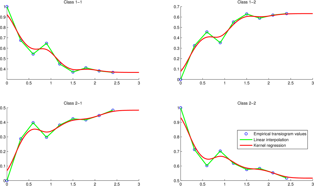
Figure 4: Non-parametric auto- and cross-transiogram models obtained via kernel regression and linear interpolation

6 Conclusions

A collection of statistical methods have been recently proposed for modeling categorical spatial data based on the concept of spatial transition probabilities. Limited discussions, however, have given to the properties of this fairly new spatial continuity measure in the existing literature. In this paper, three findings on basic properties of transiogram models are reported. Specifically, analytical connections between the shape of auto-transiograms near the origin and the spatial distribution of the associated class label was firstly revealed. Similar to variograms, it is not every function that can be used as a valid transiogram model. In the context of stationary indicator random fields, the eligibility of commonly used basic forms of variograms as transiograms was investigated particularly for the excursion sets of Gaussian random fields, one of the most commonly used random sets. It was concluded that the auto-transiogram of indicators in such a random set can not be Gaussian, Spherical, Circular or Triangular forms, which are usually used for variogram modeling. The exponential and its derived forms are recommended for transiogram modeling in the methods based on stationary indicator random fields. Finally, a non-parametric transiogram fitting procedure was proposed for the cases where the assumption of the stationary indicator random fields does not apply, to capture the small scale effects in transiograms and to address automatic joint fitting issues of transiograms as the number of classes increases. Compared to the recent joint fitting methods based on linear interpolation, the proposed kernel regression-based method is more generic and flexible, and capture the non-linear effects in empirical transiogram values naturally. A Matlab implementation of the proposed joint fitting procedure of empirical transiogram values is also provided. These three findings cover the properties, validity and modeling of transiograms, and provide a better understanding of the behaviors of transiogram models, as well as the transiogram-based methods, and thus to avoid the potential mis-use and misunderstanding of this fairly new spatial continuity measure in geographical spaces.

7 Acknowledgments

We gratefully acknowledge the funding provided by the National Geospatial-Intelligence Agency (NGA) to support this research.

References

- Allard et al. (2011) Allard, D., D’Or, D., and Froidevaux, R., 2011. An efficient maximum entropy approach for categorical variable prediction. European Journal of Soil Science, 62 (3), 381–393.
- Cao et al. (2011) Cao, G., Kyriakidis, P.C., and Goodchild, M.F., 2011. Combining spatial transition probabilities for stochastic simulation of categorical fields. International Journal of Geographical Information Science, 25 (11), 1773–1791.
- Carle and Fogg (1996) Carle, S. and Fogg, G., 1996. Transition probability-based indicator geostatistics. Mathematical Geology, 28 (4), 453–476.
- Carle and Fogg (1997) Carle, S. and Fogg, G., 1997. Modeling spatial variability with one and multidimensional continuous-lag Markov chains. Mathematical Geology, 29 (7), 891–918.
- Chilès and Delfiner (1999) Chilès, J. and Delfiner, P., 1999. Geostatistics: Modeling Spatial Uncertainty. Wiley-Interscience.
- Deutsch and Journel (1998) Deutsch, C. and Journel, A., 1998. GSLIB: Geostatistical Software Library and User’s Guide. New York, 369.
- D’Or and Bogaert (2004) D’Or, D. and Bogaert, P., 2004. Spatial prediction of categorical variables with the Bayesian maximum entropy approach: the Ooypolder case study. European Journal of Soil Science, 55 (4), 763–775.
- Emery (2010) Emery, X., 2010. On the existence of mosaic and indicator random fields with spherical, circular, and triangular variograms. Mathematical Geosciences, 42 (8), 969–984.
- Lantuejoul (2002) Lantuejoul, C., 2002. Geostatistical Simulation: Models and Algorithms. Springer Verlag.
- Li (2007a) Li, W., 2007a. Transiograms for characterizing spatial variability of soil classes. Soil Science Society of America Journal, 71 (3), 881.
- Li and Zhang (2010) Li, W. and Zhang, C., 2010. Linear interpolation and joint model fitting of experimental transiograms for Markov chain simulation of categorical spatial variables. International Journal of Geographical Information Science, 24 (6), 821–839.
- Li (2006) Li, W., 2006. Transiogram: A spatial relationship measure for categorical data. International Journal of Geographical Information Science, 20 (6), 693–699.
- Li (2007b) Li, W., 2007b. Markov chain random fields for estimation of categorical variables. Mathematical Geology, 39 (3), 321–335.
- Li and Zhang (2006) Li, W. and Zhang, C., 2006. A generalized Markov chain approach for conditional simulation of categorical variables from grid samples. Transactions in GIS, 10 (4), 651–669.
- Li et al. (2011) Li, W., Zhang, C., and Dey, D.K., 2011. Modeling experimental cross-transiograms of neighboring landscape categories with the gamma distribution. International Journal of Geographical Information Science.
- Matheron (1971) Matheron, G., 1971. The Theory of Regionalized Variables and Its Applications. Vol. 5. École national supérieure des mines.
- Matheron (1993) Matheron, G., 1993. Une conjecture sur la covariance d’un ensemble aléatoire. Cahiers de geostatistique, 107, 107–113.
- McGarigal and Marks (1995) McGarigal, K. and Marks, B., FRAGSTATS: spatial pattern analysis program for quantifying landscape structure. , 1995. , Technical report PNW-GTR-351, U.S. Department of Agriculture, Forest Service, Pacific Northwest Research Station, Portland, OR.
- Nadaraya (1964) Nadaraya, E., 1964. On estimating regression. Teoriya Veroyatnostei i ee Primeneniya, 9 (1), 157–159.
- Silverman (1986) Silverman, B., 1986. Density Estimation for Statistics and Data Analysis. Chapman & Hall, CRC.
- Smith et al. (2007) Smith, M.D., Goodchild, M., and Longley, P., 2007. Geospatial Analysis: A Comprehensive Guide to Principles, Techniques and Software Tools. 2nd Troubador Publishing.
- Solow (1986) Solow, A.R., 1986. Mapping by simple indicator kriging. Mathematical Geology, 18 (3), 335–352.
- Stein (1999) Stein, M., 1999. Interpolation of Spatial Data: Some Theory for Kriging. Springer Verlag.
- Tobler (1970) Tobler, W., 1970. A computer movie simulating urban growth in the Detroit region. Economic Geography, 46 (2), 234–240.
- Tso and Mather (2001) Tso, B. and Mather, P., 2001. Classification methods for remotely sensed data. Taylor & Francis.