Effects of Long-Range Interactions on Magnetic Excitations and Phase Transition on a Magnetically Frustrated Square Lattice

Abstract

We investigate the effects of long-range interaction on the magnetic excitations and the competition between magnetic phases on a frustrated square lattice. Applying the spin wave theory and assisted with symmetry analysis, we obtain analytical expression for spin wave spectrum of competing Neel and $(\pi,0)$ stripe states of systems containing any-order long-range interactions. In the specific case of long-range interactions with power-law decay, we found surprisingly that staggered long-range interaction suppresses quantum fluctuation and enlarges the ordered moment, especially in the Neel state, and thus extends its phase boundary to the stripe state. Our findings only illustrate the rich possibilities of the roles of long-range interactions, and advocate future investigations in other magnetic systems with different structures of interactions.

I Introduction

Contrary to the well studied magnetic systems with short-range coupling, the physical effects of long-range magnetic interactions remain an important current research topic. Practically, long-range interactions are common in magnetic systems, for example with metallic carriers that mediate the interactions ohno ; apl02 , in the form of the well-known RKKY interaction rkky or the double exchange interaction yaoprl2011 . For example, the RKKY interaction has also been found on the surface of three dimensional topological insulators chenprl , where the magnetic impurities are mediated by the helical Dirac electrons. yaoprl2011 . Another current heavily debated case is the magnetic properties of iron-based superconductors, which hosts clear signal of local moment and itinerant magnetic carriers philip ; zhang09 . Obviously, in such a metallic system, if one were to integrate out the itinerant degree of freedom to obtain a spin only system, the interactions would be long-range as well. From these large classes of materials of current interest, it is obvious that a better understanding of the effects of long-range magnetic interaction is of great scientific interest and practical importance. This is particularly so when the systems contains frustrated short-range interactions and competing phases.

Previously, the effects of long-range interactions have been studied in one-dimensional systems, and found to induce various interesting phenomena, including long-range order, quasi-long range order, valence bond solid phase,etc. aoki95 ; yusuf04 ; affleck05 ; sandvik10 On the other hand, the study of effects of long-range interaction remains largely unaddressed, mainly because of technical problems.

In this paper, we investigate the effects of long-range magnetic interaction in a square lattice containing frustrated first- and second-neighbor interactions. Assisted with symmetry analysis, we derive a general analytical expression for the spin wave spectrum in the competing Neel and $(\pi,0)$ stripe states. We then study their phase competition under the influence of staggered long-range interaction with power-law decay. We found that the long-range interaction widens the spin wave spectrum, enlarges the stiffness of the spin wave, and thus suppresses the quantum fluctuation of the spin, giving rise to a larger ordered moment, particularly in the Neel state. This in turn strengthens the Neel state and extends its phase boundary to the stripe state. Our results reveal the interesting physical effects of long-range interaction in this specific frustrated system, and offer a starting point for future systematic investigations on the important role of long-range interactions in frustrated magnetic systems in general.

This paper is organized as follows. In Section II we begin with a brief description of model and method. In Section III we present the general analytical results of spin waves for both the ($\pi,\pi$) Neel phase and ($\pi,0$) stripe phase with any-order long-range interactions. In Section IV we study an adjustable long-range interaction with the form of $1/|r|^{\alpha}$. The spin wave dispersions, dynamic structure factor, constant energy slices, reduced magnetic moment and phase diagrams are obtained. Finally, in Section V we summarize the main results.

II Model and Method

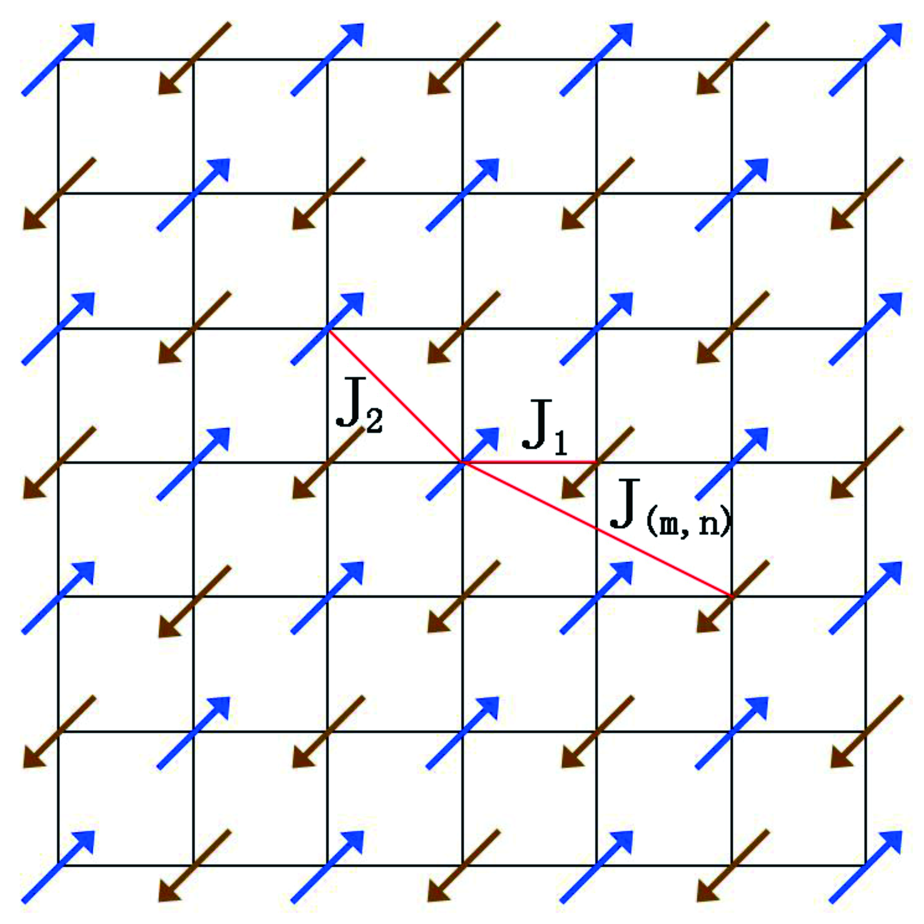
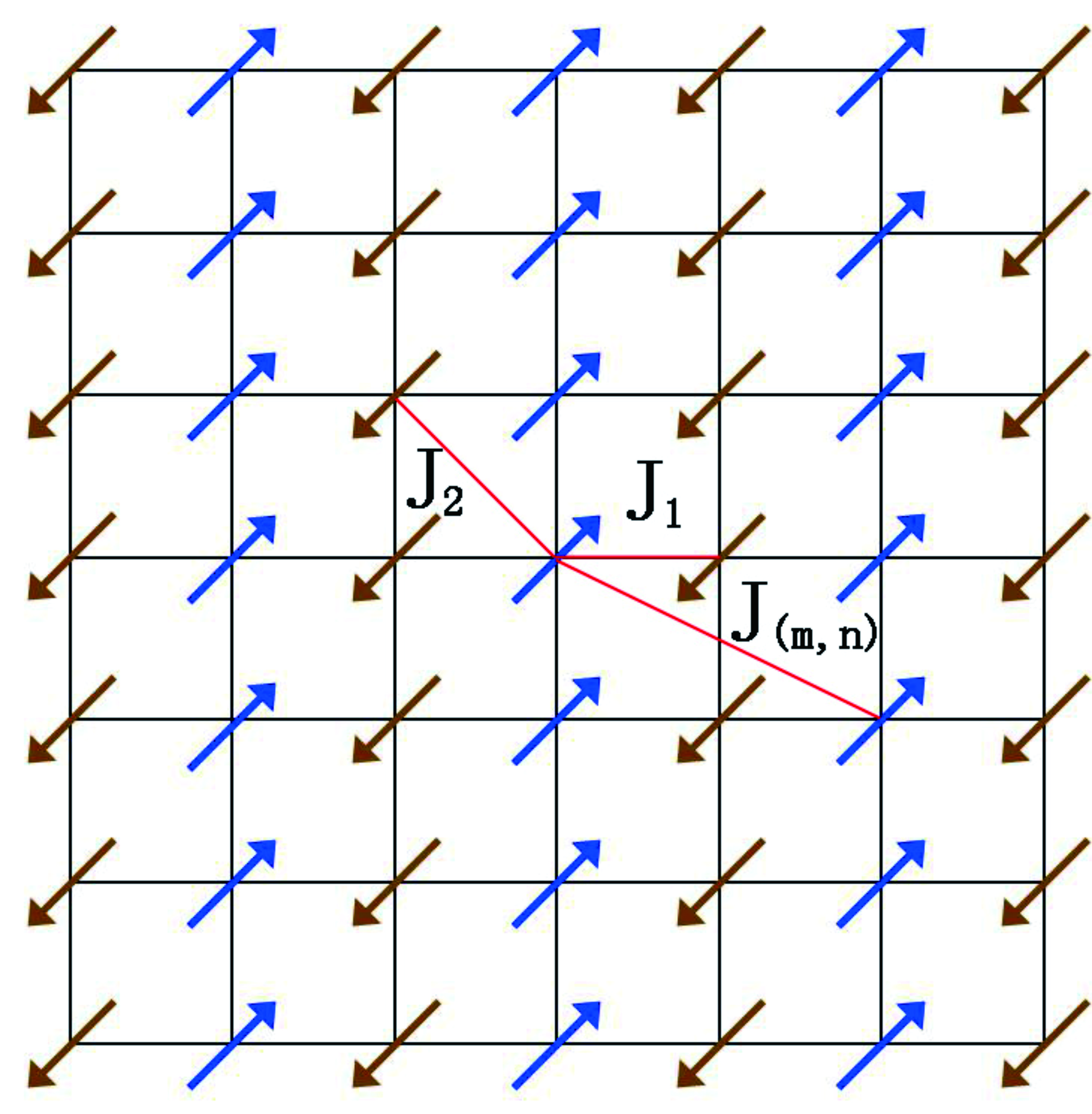
Figure 1: Magnetic ground states with long-range interactions: (a) Neel phase with wave vector ($\pi,\pi$) and (b) Stripe phase with wave vector ($\pi,0$). $J_{(m,n)}$ represents the interactions between two spins with relative coordinates $(m,n)$.

We study an extended version of the usual nearest-neighbor Heisenberg model on the two-dimensional square lattice. The Hamiltonian is written as

$$H=\sum_{<\mathbf{r},\mathbf{r^{\prime}}>}J_{\mathbf{r},\mathbf{r^{\prime}}}\mathbf{S}_{\mathbf{r}}\cdot\mathbf{S}_{\mathbf{r^{\prime}}},$$ (1)

where $<\mathbf{r},\mathbf{r^{\prime}}>$ are spin sites, and $J_{\mathbf{r},\mathbf{r^{\prime}}}$ is the exchange coupling. To describe the long-range interactions conveniently, we use $J_{\mathbf{r},\mathbf{r^{\prime}}}=J_{(m,n)}$ to represent the interaction between two spins with the relative coordinates $(m,n)$ shown in Fig. 1. For example, if we choose one site as $(0,0)$, then its neighboring sites can be coordinated by $(m,n)$, where $m$ is the relative $x$-coordinate and $n$ is the relative $y$-coordinate to the $(0,0)$-point. From this definition, we can represent $J_{1}=J_{(1,0)}$, $J_{2}=J_{(1,1)}$, $J_{3}=J_{(2,0)}$, and so on. Also we have $J_{(|m|,|n|)}=J_{(|n|,|m|)}$ by the symmetry. Therefore, we can rewrite the Hamitonian as

$$H = \sum_{<\mathbf{r},\mathbf{r^{\prime}}>}J_{(m,n)}\mathbf{S}_{\mathbf{r}}\cdot\mathbf{S}_{\mathbf{r^{\prime}}},$$ (2)

where $J_{(m,n)}$ depends on the relative coordinates between $\mathbf{S}_{\mathbf{r}}$ and $\mathbf{S}_{\mathbf{r^{\prime}}}$.

By tuning the interactions, the system can be in the $(\pi,\pi)$ antiferromagnetic phase (see Fig. 1) and $(\pi,0)$ antiferromagnetic phase (see Fig. 1). The $(\pi,\pi)$ antiferromagnetic phase is the ground state of undoped cuprates, and $(\pi,0)$ antiferromagnetic phase is closely related to iron pnictides. dai08 ; zhao09 ; ma09 There are two spins in each unit cell for these two antiferromagnetic phases.

We use Holstein-Primakoff bosons to quantize about the antiferromagnetic ground states.

$$H=E_{Cl}+S\sum_{\mathbf{k}}[A_{\mathbf{k}}a_{\mathbf{k}}^{+}a_{\mathbf{k}}+\frac{1}{2}(B_{\mathbf{k}}a_{\mathbf{k}}^{+}a_{-\mathbf{k}}^{+}+B_{\mathbf{-k}}^{*}a_{\mathbf{k}}a_{-\mathbf{k}}]$$ (3)

where $E_{Cl}$ is the classical ground state energy which depends on the spin configuration and interactions.

The Hamiltonian can be diagonalized using the Bogoliubov transformation erica04

$$b_{\mathbf{k}}=\cosh{\theta_{\mathbf{k}}a_{\mathbf{k}}}-\sinh{\theta_{\mathbf{k}}}a_{-\mathbf{k}}^{+}.$$ (4)

The diagonalized Hamiltonian is

$$H=\sum_{\mathbf{k}}\omega(\mathbf{k})b_{\mathbf{k}}^{+}b_{\mathbf{k}}+E_{Cl}+E_{0}$$ (5)

where $\omega(\mathbf{k})$ is the spin wave dispersion

$$\omega(\mathbf{k})=S\sqrt{A_{\mathbf{k}}^{2}-B_{\mathbf{k}}^{2}},$$ (6)

and $E_{0}$ is the quantum zero-point energy correction

$$E_{0}=\frac{S}{2}\sum_{\mathbf{k}}(-A_{\mathbf{k}}+\omega(\mathbf{k})).$$ (7)

The dynamic structure factor $S(\mathbf{k},\omega)$ is an important quantity which is proportional to the neutron scattering cross section. In the linear spin-wave approximation, only the transverse parts contribute to the dynamic structure factor. We have

$$S^{xx}(\mathbf{k},\omega) = S^{yy}(\mathbf{k},\omega)$$

$$= g^{2}\mu_{B}^{2}S\frac{A_{k}-B_{k}}{2\omega(\mathbf{k})}[n(\omega)+1]\delta(\omega-\omega(\mathbf{k})),$$

where $g$ is the $g$-factor, and $n(\omega)$ is the Bose occupation factor. yaofront09 ; boothroyd08

III Analytical Results

Through the linear spin wave theory as mentioned in Section II, we obtain the analytical results for both the Neel phase and stripe phase with long-range interactions. The spin wave dispersion is given by

$$\omega(\mathbf{k})=S\sqrt{A_{\mathbf{k}}^{2}-B_{\mathbf{k}}^{2}},$$ (9)

where

$$A_{\mathbf{k}} = \sum_{(m,n)}A_{(m,n)},$$ (10)

$$B_{\mathbf{k}} = \sum_{(m,n)}B_{(m,n)}.$$ (11)

Here $A_{(m,n)}$ and $B_{(m,n)}$ depend on the symmetry of ground state and will be given separately.

III.1 $(\pi,\pi)$ Neel phase

According to the geometric structure of $(\pi,\pi)$ antiferromagnet with any order long-range interactions, we find that

$$A_{(m,n)} = 4{(-1)}^{m+n+1}\alpha(m,n)J_{(m,n)}$$

$$+ [{(-1)}^{m+n}+1]\alpha(m,n)J_{(m,n)}$$

$$[\cos{(mk_{x})}\cos{(nk_{y})}+\cos{(nk_{x})}\cos{(mk_{y})}],$$

$$B_{(m,n)} = [{(-1)}^{m+n+1}+1]\alpha(m,n)J_{(m,n)}$$

$$[\cos{(mk_{x})}\cos{(nk_{y})}+\cos{(nk_{x})}\cos{(mk_{y})}].$$

Here we have defined

$$\alpha(m,n)=\left\{\begin{array}[]{*{20}{c}}&1&&{m=0}~{}or~{}{n=0}~{}or~{}{m=n}\\ &2&&{otherwise}\end{array}\right.$$ (14)

The coefficients in Eqs. (III.1) and (III.1) are determined by the direction of spins. In the Neel phase, we find that $(m+n)$ is always even if the spin at $(m,n)$ has the same direction with the one at $(0,0)$, otherwise it is odd. $\alpha(m,n)$ is $1$ if the spins are located at the high symmetry points, i.e. ${m=0}~{}or~{}{n=0}~{}or~{}{m=n}$; otherwise it is $2$.

In the case of $|m|=1$ and $|n|=0$, we recover the classical result for the $J_{1}$-only model on the square lattice  kruger

$$A_{\mathbf{k}} = 4J_{1}$$ (15)

$$B_{\mathbf{k}} = 2J_{1}[\cos{(k_{x})}+\cos{(k_{y})}]$$ (16)

In the case of $|m|\leq 1$ and $|n|\leq 1$, which has no long-range interaction, we have

$$A_{\mathbf{k}} = 4(J_{1}-J_{2})+4J_{2}\cos{(k_{x})}\cos{(k_{y})}$$ (17)

$$B_{\mathbf{k}} = 2J_{1}[\cos{(k_{x})}+\cos{(k_{y})}]$$ (18)

From this expression, we can see that the spin wave dispersion is invariant if we switch $k_{x}$ and $k_{y}$ even the long-range interactions are included. This reflects the symmetry of $(\pi,\pi)$ phase.

III.2 $(\pi,0)$ Stripe phase

For the $(\pi,0)$ antiferromagnet with long-range interactions, the spin wave dispersion is also given by Eqs. (9),(10)and(11). We have found

$$A_{(m,n)} = 2{(-1)}^{m+1}|{(-1)}^{m}+{(-1)}^{n}|\alpha(m,n)J_{(m,n)}$$ (19)

$$+ \alpha(m,n)J_{(m,n)}\{[{(-1)}^{m}+1]\cos{(mk_{x})}\cos{(nk_{y})}$$

$$+ [{(-1)}^{n}+1]\cos{(nk_{x})}\cos{(mk_{y})}\},$$

$$B_{(m,n)} = \alpha(m,n)J_{(m,n)}\{[{(-1)}^{m+1}+1]\cos{(mk_{x})}\cos{(nk_{y})}$$ (20)

$$+ [{(-1)}^{n+1}+1]\cos{(nk_{x})}\cos{(mk_{y})}\}.$$

In the stripe phase, $m$ is even if the spin at $(m,n)$ has the same direction with the one at $(0,0)$, otherwise it is odd. Its spin wave band is quite different from the Neel phase.

When considering the case with $|m|\leq 1$ and $|n|\leq 1$, we can get

$$A_{\mathbf{k}} = 2J_{1}\cos{(k_{y})}+4J_{2}$$ (21)

$$B_{\mathbf{k}} = 2J_{1}\cos{(k_{x})}+4J_{2}\cos{(k_{x})}\cos{(k_{y})},$$ (22)

which is exactly the same result of $J_{1}$-$J_{2}$ model. yao08J1J2 ; si08 ; fang08

This spin wave dispersion is asymmetric if we switch $k_{x}$ and $k_{y}$. This reflects the symmetry of $(\pi,0)$ phase.

To get the dynamic structure factor, we just need to substitute the $A_{K}$ and $B_{k}$ obtained above into Eq. (LABEL:strfactor).

With the above analytic solutions, we can easily explore the spin wave dispersions, spin wave velocities, dynamic structure factor, reduced magnetic moment and phase transitions for the $(\pi,\pi)$ Neel antiferromagnet and $(\pi,0)$ stripe antiferromagnet with all kinds of long-range interactions. In the following Section, we will use an adjustable power-law long-range interaction to study the magnetic excitations and phase transition.

IV Power-law long-range interactions

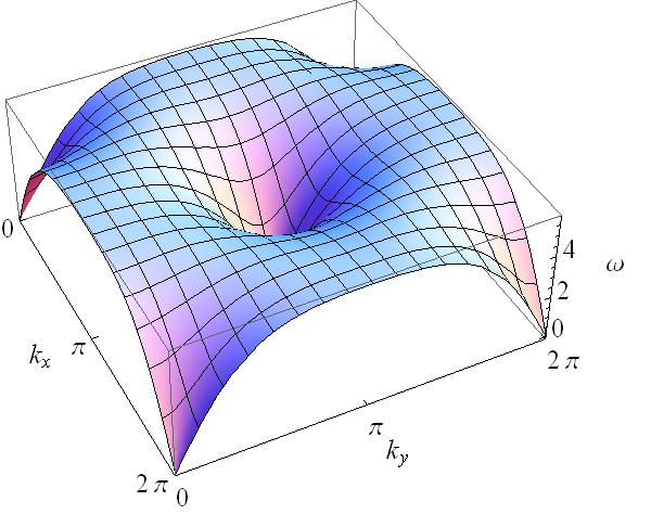
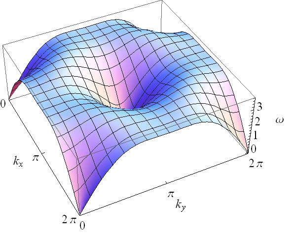
Figure 2: (Color online) Spin-wave dispersion band for the $(\pi,\pi)$ Neel phase with $J_{2}=0.1$, $J_{1}=1$: (a) $\alpha=4$ (long-range interactions) and (b) $\alpha=10$ (short range interactions).

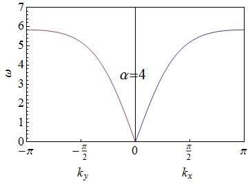
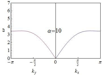
Figure 3: (Color online) Spin-wave dispersions for the $(\pi,\pi)$ Neel phase with $J_{2}=0.1$, $J_{1}=1$: (a) $\alpha=4$ (long-range interactions and (b) $\alpha=10$ (short range interactions). The spin wave velocities $v_{x}$ and $v_{y}$ increase about $80\%$ from $\alpha=10$ to $4$.

In this section, we study the long-range interactions which decay as a power law $1/|r|^{\alpha}$:

$$J_{(m,n)} = {\left({-1}\right)^{\left|m\right|+\left|n\right|+1}}\frac{{\lambda{J_{1}}}}{{{{|r|}^{\alpha}}}}$$ (23)

$$= {\left({-1}\right)^{\left|m\right|+\left|n\right|+1}}\frac{{\lambda{J_{1}}}}{{{{(\sqrt{{m^{2}}+{n^{2}}})}^{\alpha}}}},$$

where $\lambda$ denotes the relative strength compared to $J_{1}$ and $\alpha$ is the power-law exponent that controls the decay of interactions. The factor $(-1)^{|m|+|n|+1}$ ensures that the interactions are not frustrated. aoki95 ; yusuf04 Experimentally, this kind of power-law long-range interactions can be realized by the RKKY interactions where local magnetic ions are mediated by the itinerant electrons. rkky Theoretically, this type of long-range interactions can be simulated by quantum monte carlo methods without the notorious sign problem. sandvik10 In this Section, we use a circle of spins (61) which satisfy $\sqrt{m^{2}+n^{2}}\leq 3\sqrt{2}$ as an illustration. We also calculated the cases for $\sqrt{m^{2}+n^{2}}>3\sqrt{2}$, which shows no difference when $\alpha\geq 2$.

Shown in Fig. 1, we have $r={(\sqrt{{m^{2}}+{n^{2}}})}$. The corresponding interactions can be obtained from Eq. (23). Here, we use

$$J_{2}^{{}^{\prime}}=J_{2}-\frac{\lambda J_{1}}{\sqrt{2}^{\alpha}},$$ (24)

where a NNN interaction $J_{2}$ is added together with the power-law interaction to introduce the competition. The new $J_{2}^{{}^{\prime}}$ includes both $J_{2}$ and power-law term, which can be substituted into previous formulas. We will see that $J_{2}$ is an important parameter to control the phase transition. In the following, we will use $\lambda=1$ for calculations.

IV.1 $(\pi,\pi)$ Neel phase

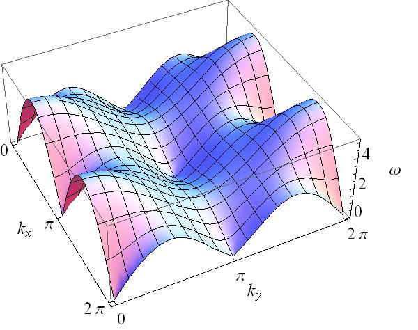
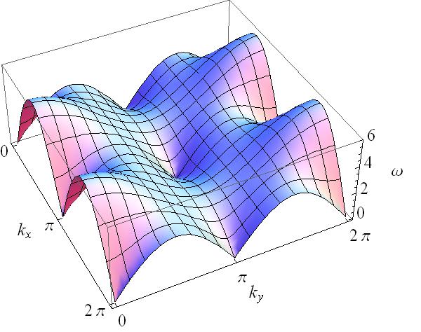
Figure 4: (Color online) Spin-wave dispersion band for the $(\pi,0)$ stripe phase with $J_{2}=1$, $J_{1}=1$: (a) $\alpha=4$ (long-range interactions) and (b) $\alpha=10$ (Short range interactions).

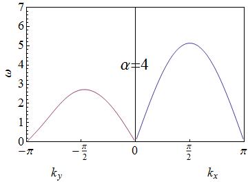
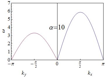
Figure 5: (Color online) Spin-wave dispersions for the $(\pi,0)$ stripe phase with $J_{2}=1$, $J_{1}=1$: (a) $\alpha=4$ (long-range interactions) and (b) $\alpha=10$ (short range interactions). The spin wave velocity $v_{x}$ decreases about $13\%$ and $v_{y}$ drops about $20\%$ from $\alpha=10$ to $4$.

By substituting the above power-law long-range interactions into Eqs. (10) and (11), we can get the spin wave dispersion

$$A_{\mathbf{k}} = 4(\lambda J_{1}/\sqrt{2}^{\alpha}-J_{2})+4(\lambda J_{1}/\sqrt{8}^{\alpha})+4(\lambda J_{1}/\sqrt{18}^{\alpha})$$ (25)

$$+ 4(\lambda J_{1}/2^{\alpha})+8(\lambda J_{1}/\sqrt{10}^{\alpha})+4J_{1}+8(\lambda J_{1}/\sqrt{5}^{\alpha})$$

$$+ 8(\lambda J_{1}/\sqrt{13}^{\alpha})+4(\lambda J_{1}/3^{\alpha})+4(\lambda J_{1}/4^{\alpha})$$

$$+ 8(\lambda J_{1}/\sqrt{17}^{\alpha})$$

$$- 4(\lambda J_{1}/\sqrt{2}^{\alpha}-J_{2})\cos{(k_{x})}\cos{(k_{y})}$$

$$- 4\lambda J_{1}/\sqrt{8}^{\alpha}\cos{(2k_{x})}\cos{(2k_{y})}$$

$$- 4\lambda J_{1}/\sqrt{18}^{\alpha}\cos{(3k_{x})}\cos{(3k_{y})}$$

$$- 2\lambda J_{1}/2^{\alpha}[\cos{(2k_{x})}+\cos{(2k_{y})}]$$

$$- 4\lambda J_{1}/\sqrt{10}^{\alpha}[\cos{(3k_{x})}\cos{(k_{y})}+\cos{(k_{x})}\cos{(3k_{y})}]$$

$$- 2\lambda J_{1}/4^{\alpha}[\cos{(4k_{x})}+\cos{(4k_{y})}]$$

$$B_{\mathbf{k}} = 2J_{1}[\cos{(k_{x})}+\cos{(k_{y})}]+2\lambda J_{1}/3^{\alpha}[\cos{(3k_{x})}+\cos{(3k_{y})}]$$ (26)

$$+ 4\lambda J_{1}/\sqrt{5}^{\alpha}[\cos{(2k_{x})}\cos{(k_{y})}+\cos{(k_{x})}\cos{(2k_{y})}]$$

$$+ 4\lambda J_{1}/\sqrt{13}^{\alpha}[\cos{(3k_{x})}\cos{(2k_{y})}+\cos{(2k_{x})}\cos{(3k_{y})}]$$

$$+ 4\lambda J_{1}/\sqrt{17}^{\alpha}[\cos{(4k_{x})}\cos{(k_{y})}+\cos{(k_{x})}\cos{(4k_{y})]}$$

Fig. 2 shows the spin wave band with different interactions for the $(\pi,\pi)$ Neel phase. The spin wave band with long-range interactions is shown in Fig. 2 for $J_{2}=0.1$ and $\alpha=4$. The other one with short range interactions is shown in Fig. 2 for $J_{2}=0.1$ and $\alpha=10$. From the plots, we can see that the low energy spin wave bands are almost invariant for the two kinds of interactions. Both bands have $\omega\rightarrow 0$ at $(\pi,\pi)$ point which corresponds to the magnetic wave vector. However, the difference shows up at high energies: different band shapes and energy scales. This reflects the geometry of interactions.

The associated spin wave velocities are

$$v_{x}=v_{y}=2\sqrt{2}S\sqrt{(J_{1}-2J_{2}+a_{1}\lambda J_{1})(J_{1}+b_{1}\lambda J_{1})},$$ (27)

where
$\begin{array}[]{l}{a_{1}}={2^{1-\frac{\alpha}{2}}}+{2^{2-\alpha}}+{2^{3-\frac{{3\alpha}}{2}}}+{3^{2-\alpha}}+{2^{1-\frac{\alpha}{2}}}\times{3^{2-\alpha}}\\ ~{}~{}~{}+2\times{5^{1-\frac{\alpha}{2}}}+{2^{2-\frac{\alpha}{2}}}\times{5^{1-\frac{\alpha}{2}}}+2\times{13^{1-\frac{\alpha}{2}}}+2\times{17^{1-\frac{\alpha}{2}}}\\ {a_{2}}={3^{-\alpha}}+2\times{5^{-\frac{\alpha}{2}}}+2\times{13^{-\frac{\alpha}{2}}}+2\times{17^{-\frac{\alpha}{2}}}\end{array}$

When $\alpha\rightarrow\infty$, we have

$$v_{x}=v_{y}=2\sqrt{2}S\sqrt{J_{1}(J_{1}-2J_{2})},$$ (28)

From this equation, we can see that there is a phase transition at $J_{2}=0.5J_{1}$ for the $J_{1}$-$J_{2}$ model.

The spin wave velocities along $k_{x}$- and $k_{y}$-directions are the same because of the symmetry of $(\pi,\pi)$ phase. Fig. 3 shows the velocities (slope) along $k_{x}$- and $k_{y}$-directions at the point $(0,0)$ in the $k$ space. It can be seen that the long-range interactions increase the spin wave velocities $v_{x}$ and $v_{y}$ dramatically in the $(\pi,\pi)$ Neel phase, see Fig. 3.

IV.2 $(\pi,0)$ Stripe phase

The stripe phase by definition is not only breaking the spin rotational symmetry but also breaks the crystal $C_{4}$ symmetry down to $C_{2}$. Substituting the same power law form of long-range interactions into Eqs. (10) and (11), we can get the spin wave dispersion for the $(\pi,0)$ stripe phase:

$$A_{\mathbf{k}} = 4(J_{2}-\lambda J_{1}/\sqrt{2}^{\alpha})+4\lambda J_{1}/\sqrt{8}^{\alpha}-4\lambda J_{1}/\sqrt{1}8^{\alpha}$$ (29)

$$+ 4\lambda J_{1}/2^{\alpha}-8\lambda J_{1}/\sqrt{10}^{\alpha}+4\lambda J_{1}/4^{\alpha}$$

$$- 4\lambda J_{1}/\sqrt{8}^{\alpha}\cos{(2{k_{x}})}\cos{(2{k_{y})}}$$

$$- 2\lambda J_{1}/2^{\alpha}[\cos{(2{k_{x}})}+\cos{(2{k_{y}})}]$$

$$+ 2J_{1}\cos{(k_{y})}+4\lambda J_{1}/\sqrt{5}^{\alpha}\cos{(k_{y})}\cos{(2{k_{x})}}$$

$$+ 4\lambda J_{1}/\sqrt{13}^{\alpha}\cos{(3k_{y})}\cos{(2{k_{x}})}+2\lambda J_{1}/3^{\alpha}\cos{(3{k_{y}})}$$

$$- 2\lambda J_{1}/4^{\alpha}[\cos{(4k_{x})}+\cos{(4k_{y})}]$$

$$+ 4\lambda J_{1}/\sqrt{17}^{\alpha}\cos{(k_{y})}\cos{(4k_{x})}$$

$$B_{\mathbf{k}} = 4(J_{2}-\lambda J_{1}/\sqrt{2}^{\alpha})\cos{(k_{x})}\cos{(k_{y})}$$ (30)

$$- 4\lambda J_{1}/\sqrt{18}^{\alpha}\cos{(3k_{x})}\cos{(3k_{y})}$$

$$- 4\lambda J_{1}/\sqrt{10}^{\alpha}[\cos{(3{k_{x}})}\cos{(k_{y})}+\cos{(k_{x})}\cos{(3{k_{y})}}]$$

$$+ 2{J_{1}}\cos{(k_{x})}+4\lambda J_{1}/\sqrt{5}^{\alpha}\cos{(2{k_{y})}}\cos{(k_{x})}$$

$$+ 4\lambda J_{1}/\sqrt{13}^{\alpha}\cos{(2{k_{y})}}\cos{(3{k_{x}})}+2\lambda J_{1}/3^{\alpha}\cos{(3{k_{x}})}$$

$$+ 4\lambda J_{1}/\sqrt{17}^{\alpha}\cos{(4k_{y})}\cos{(k_{x})}$$

Fig. 4 shows the spin wave band for the $(\pi,0)$ stripe phase. It is very different from the $(\pi,\pi)$ Neel phase because of the different symmetry.

Here we use $J_{2}=1$ in the $(\pi,0)$ stripe phase, which is much larger than that in the $(\pi,\pi)$ Neel phase required by the stability of ground state. Comparing Fig. 4 with Fig. 4, we can see that the long-range interactions here reduce the energy instead of increasing the energy in the $(\pi,\pi)$ Neel phase. It is because the long-range interactions here decrease the stability of $(\pi,0)$ stripe phase. We will get to this point in the following part.

We can get the associated spin wave velocities

$$v_{x} = 2S\{[2J_{2}+J_{1}(1-a_{3}\lambda)]$$

$$(2J_{2}+J_{1}(1-a_{4}\lambda))\}^{1/2}$$

$$v_{y} = 2S\{[2J_{2}+J_{1}(a_{5}\lambda-1)]$$ (31)

$$(2J_{2}+J_{1}(1-a_{4}\lambda))\}^{1/2}$$

where
$\begin{array}[]{l}{a_{3}}=-2^{1-\frac{\alpha}{2}}+2^{2-\alpha}+2^{3-\frac{3\alpha}{2}}+3^{2-\alpha}-2^{1-\frac{\alpha}{2}}\times 3^{2-\alpha}\\ +4^{2-\alpha}-2^{2-\frac{\alpha}{2}}\times 5^{1-\frac{\alpha}{2}}-6\times 5^{-\frac{\alpha}{2}}+10\times 13^{-\frac{\alpha}{2}}-30\times 17^{-\frac{\alpha}{2}}\\ {a_{4}}=2^{1-\frac{\alpha}{2}}-3^{-\alpha}+2^{1-\frac{\alpha}{2}}\times 3^{-\alpha}-2\times 5^{-\frac{\alpha}{2}}+2^{2-\frac{\alpha}{2}}\times 5^{-\frac{\alpha}{2}}\\ -2\times 13^{-\frac{\alpha}{2}}-2\times 17^{-\frac{\alpha}{2}}\\ {a_{5}}=-2^{1-\frac{\alpha}{2}}+2^{2-\alpha}+2^{3-\frac{3\alpha}{2}}+3^{2-\alpha}-2^{1-\frac{\alpha}{2}}\times 3^{2-\alpha}\\ +4^{2-\alpha}-2^{2-\frac{\alpha}{2}}\times 5^{1-\frac{\alpha}{2}}+6\times 5^{-\frac{\alpha}{2}}-10\times 13^{-\frac{\alpha}{2}}+30\times 17^{-\frac{\alpha}{2}}\\ \end{array}$

When $\alpha\rightarrow\infty$, we can get

$$v_{x} = 2S|2J_{2}+J_{1}|,$$ (32)

$$v_{y} = 2S\sqrt{4{J_{2}}^{2}-J_{1}^{2}}.$$ (33)

which are the results of $J_{1}$-$J_{2}$ model on the $(\pi,0)$ stripe phase. yao08J1J2 We find that the spin wave velocity $v_{x}$ decreases about $13\%$ and $v_{y}$ drops about $20\%$ from the short-range interaction case ($\alpha=10$) to the long-range interaction case $\alpha=4$).

The velocities along $k_{x}$- and $k_{y}$-directions are different and have more complicated forms than that in the $(\pi,\pi)$ Neel phase. to the long-range interaction case ($\alpha=10$). First, the $(\pi,0)$ stripe phase is asymmetric along the $k_{x}$- and $k_{y}$-directions. The system is antiferromagnetic along $x$-direction and ferromagnetic along $y$-direction. Second, we find that $v_{x}$ is always larger than $v_{y}$, and the long-range interactions reduce the spin wave velocities because they weaken the $(\pi,0)$ stripe phase instead of enhancing the $(\pi,\pi)$ Neel phase. Here only $J_{2}$ holds the $(\pi,0)$ stripe phase.

IV.3 Constant energy slices

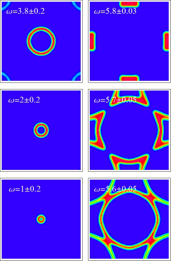
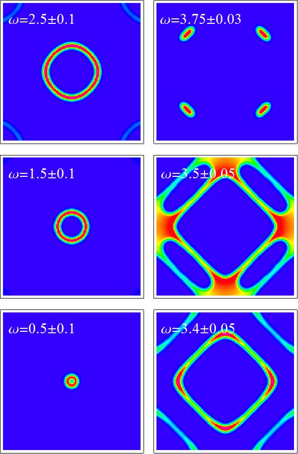
Figure 6: (Color online) Constant-energy slices (twinned) of the dynamic structure factor $S(\mathbf{k},\omega)$ for $J_{2}=0.1$, $J_{1}=1$, $\lambda=1$: (a) $\alpha=4$ (long-range interactions) and (b) $\alpha=10$ (short range interactions). The x-axis and y-axis correspond to $k_{x}$ and $k_{y}$ respectively with the range $(0,2\pi)$.

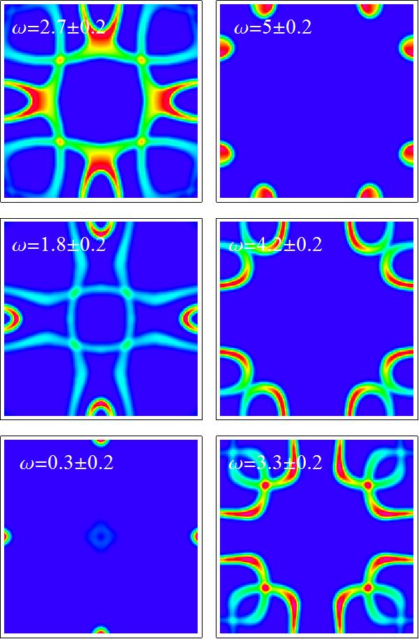
Figure 7: (Color online) Constant-energy slices (twinned) of the dynamic structure factor $S(\mathbf{k},\omega)$ for $J_{2}=1$, $J_{1}=1$, $\lambda=1$: (a) $\alpha=4$ (long-range interactions) and (b) $\alpha=10$ (short range interactions). The x-axis and y-axis correspond to $k_{x}$ and $k_{y}$ respectively with the range $(0,2\pi)$.

To compare with neutron scattering experiments, we calculate the constant energy slices. In Figs. 6 and 7, we show the twinned neutron scattering intensity plots at constant energy for the dynamic structure factor $S(\mathbf{k},\omega)$ in $\mathbf{k}$-space, assuming a crystal with twinned $(\pi,\pi)$ antiferromagnetic domains (Fig. 6) or $(\pi,0)$ antiferromagnetic domains (Fig. 7). In real materials, spin order is generally twinned because of crystal twining and local disorder pinning. yao06 ; yao08a ; boothroyd09 For this reason, we show the twinned constant energy cutting plots which can be detected by inelastic neutron scattering experiment.

For the $(\pi,\pi)$ Neel phase, there is a main peak located at $(\pi,\pi)$ at low energy for both the long-range interactions (Fig. 6) and short range interactions (Fig. 6), which corresponds to the magnetic wave vector of Neel phase. As energy increases, the peak increases quickly to an outer ring. At higher energy, the ring forms bright spots and they touch each other.

However, there is a clear difference between the long-range interactions and short range interactions at high energies. For example, the central ring is almost a circle at high energy, while it is a square for the short range interactions. This is because the long-range interactions bring more symmetry to the system. For the case with long-range interactions, the peaks are located at $(0,\pi)$, $(\pi,0)$, $(2\pi,\pi)$ and $(\pi,2\pi)$. In the second case, the band tops are located at $(\pi/2,\pi/2)$, $(\pi/2,3\pi/2)$, $(3\pi/2,\pi/2)$ and $(3\pi/2,3\pi/2)$. In addition, we find that the long-range interactions raises the top of energy while keeping other parameters the same.

For the $(\pi,0)$ stripe phase, we show the constant energy slices with $\alpha=4$ and $\alpha=10$ (Fig. 7). At low energy, there is one diffraction peak located at $(\pi,0)$, which is the magnetic wave vector of the stripe phase. Unlike the $(\pi,\pi)$ Neel phase, the low energy spin wave cones are generally elliptical. At higher energies, the peaks are located at $(\pi/2,0)$, $(0,\pi/2)$ and the symmetry related points (see Figs. 7 and  7). Contrary to the We notice that the neutron scattering patterns are not sensitive to the long-range interactions. However, the long-range interactions can decrease the band top rather than increasing it because they try to destroy the $(\pi,0)$ phase.

IV.4 Reduced magnetic moment

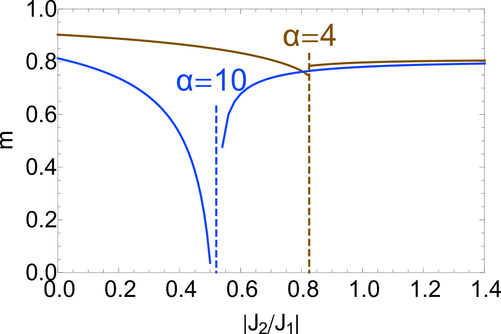
Figure 8: (Color online) $|J_{2}/J_{1}|$ dependence of $m$ for $|J_{1}|=1$, $\lambda=1$ and $S=1$. Blue is for $\alpha=10$ (long-range interactions) and brown is for $\alpha=4$ (short range interactions).

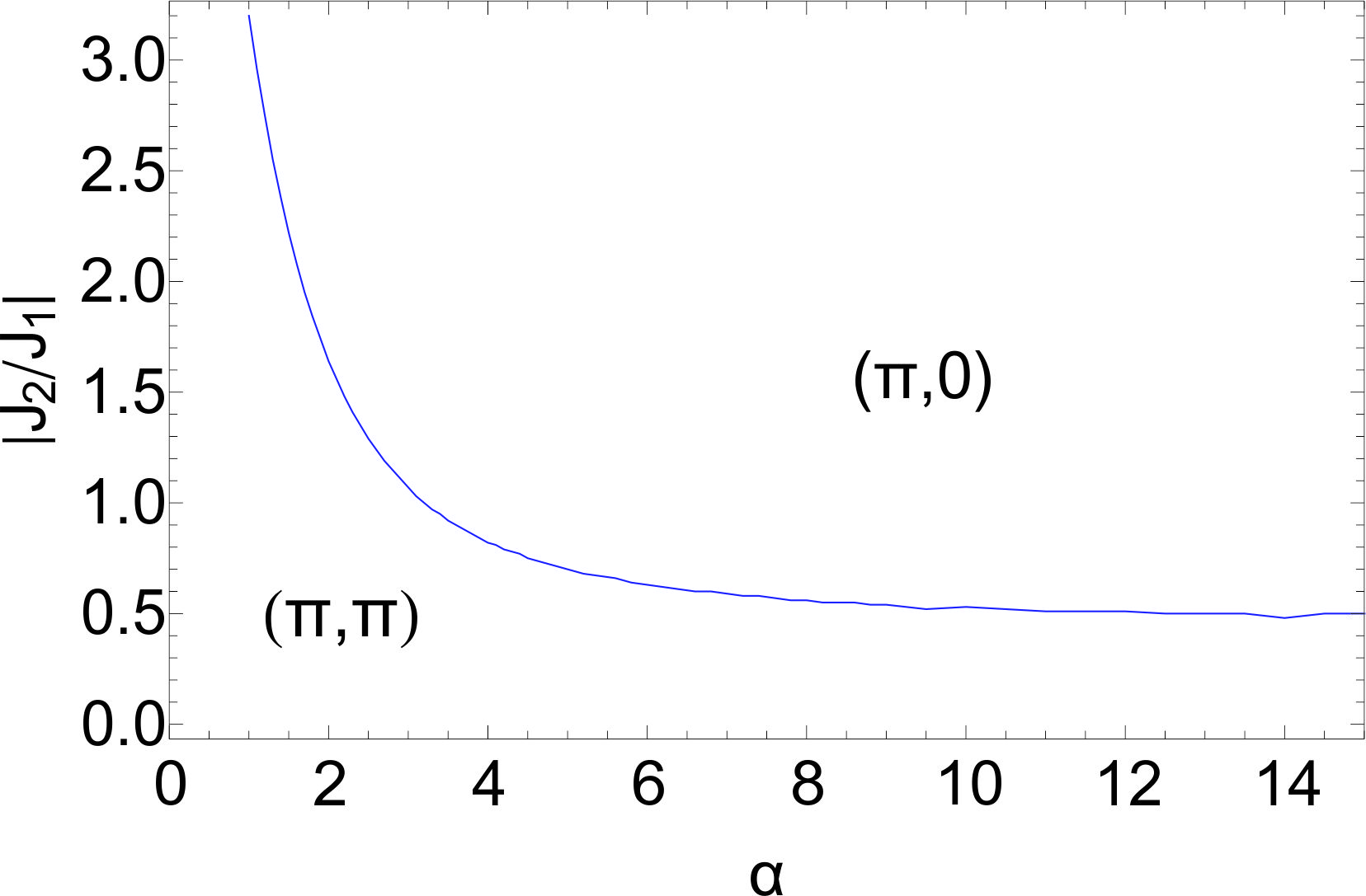
Figure 9: Phase transition point vs. $\alpha$ with $J_{1}=1$ and $\lambda=1$.

In the spin wave theory, both the quantum zero point fluctuations and thermal fluctuations can reduce the magnetic moment. The sublattice magnetization $m$ is defined as

$$m=<S_{i}^{Z}>=S-\Delta m,$$ (34)

where $\Delta m$ is the deviation of sublattice magnetization from the saturation value,

$$\Delta m = <a_{i}^{+}a_{i}>$$ (35)

$$= \sum_{\mathbf{k}}<a_{\mathbf{k}}^{+}a_{\mathbf{k}}>$$

$$= \frac{1}{2V_{\mathbf{k}}}\sum_{\mathbf{k}}[\frac{SA_{\mathbf{k}}}{\omega(\mathbf{k})}-1]+\frac{1}{V_{\mathbf{k}}}\sum_{\mathbf{k}}\frac{SA_{\mathbf{k}}}{\omega(\mathbf{k})}\frac{1}{e^{\beta\omega(\mathbf{k})}-1}$$

$$= \Delta m^{quantum}+\Delta m^{thermal}.$$

The first term $\Delta m^{quantum}$ comes from the quantum zero point fluctuations and the second term $\Delta m^{thermal}$ corresponds to the thermal fluctuations. Experimentally, the thermal fluctuations at low temperature are generally weak and can be ignored. keimer08 ; boothroyd08 ; canfield10 In the present paper, we focus on the quantum zero point fluctuations.

The sublattice magnetization $\Delta m^{quantum}$ can be calculated by  yaofront09

$$\Delta m^{quantum}=\frac{1}{2}\int_{0}^{2\pi}\int_{0}^{2\pi}\frac{dk_{x}}{2\pi}\frac{dk_{y}}{2\pi}\frac{SA_{\mathbf{k}}}{\omega(\mathbf{k})}-\frac{1}{2}.$$ (36)

It is difficult to get the analytical form of $\Delta m^{quantum}$. Thus we numerically calculate $\Delta m^{quantum}$ and $m$.

In Fig. 8, $m$ is plotted as a function of interaction ratio $|J_{2}/J_{1}|$ for $S=1$. When $\alpha$ is big enough, for example, $\alpha=10$, which corresponds to the short range interactions, $m$ drops to $0$ at the point $|J_{2}/J_{1}|\approx 0.5$ and the phase transition happens. This result is consistent with the $J_{1}$-$J_{2}$ model. When long-range interactions are introduced, the phase transition point shifts to the right. For example, it becomes $\sim 0.825$ when $\alpha=4$, shown in Fig. 8. From the sharpness of $m$ near the transition point, we can see that staggered long-range interactions suppresses quantum fluctuations of spins and enlarges the ordered moment, especially in the Neel state.

IV.5 Phase transition

There is a competition between the $(\pi,\pi)$ Neel phase and $(\pi,0)$ stripe phase. From the reduced magnetic moment, we get a phase diagram (see Fig. 9) for the competing Neel and $(\pi,0)$ stripe states of system containing first- and second-neighbor interactions, in the presence of staggered power-law interactions. The phase transition point is plotted as a function of $\alpha$, which controls the long-range interactions. It can be found that the $(\pi,\pi)$ Neel phase is below the transition line, while the $(\pi,0)$ stripe phase is above it. As $\alpha$ increases, the phase transition point ($|J_{2}/J_{1}|$) decreases quickly and saturates at $0.5$, recovering the result of $J_{1}$-$J_{2}$ model. When $\alpha$ approaches $1$, i.e. the interactions decay slowly, the phase transition point $|J_{2}/J_{1}|$ increases to $\sim 3.21$ if the longest $J_{(m,n)}=J_{(3,3)}$.

V Conclusions

In conclusion, we have studied the magnetic excitations and phase transition on the square lattice with long-range interactions, which are related to the cuprate superconductors and iron-based superconductors. The general solutions of spin waves have been worked out for the system with any-order long-range interactions for the $(\pi,\pi)$ Neel phase and $(\pi,0)$ stripe phase. Particulary, for the system with power-law long-range interactions, we have calculated the spin wave dispersions, spin wave velocities, dynamic structure factor, constant energy cutting plots, reduced magnetic moment and phase diagram. The spin wave cones at the $(\pi,\pi)$ Neel phase are found to be more circular at low energies because of the existence of long-range interactions. At the $(\pi,0)$ stripe phase, the spin wave cones are general elliptical at low energies and the long-range interactions suppress the whole energy band. At high energies, the long-range interactions have the obvious effect to the magnetic excitations which can be measured by the inelastic neutron scattering, NMR, $\mu$SR, etc. The remarked calculated magnetic moment can be used to examine the effects of long-range interactions in real materials. We have found surprisingly that staggered long-range interaction can shift the phase transition point and suppress the quantum fluctuation of spin and enlarges the ordered moment,especially in the Neel state. Our study provides very general results for the two-dimensional square lattice with long-range interactions, which can be used by both theoretical and experimental studies.

- (1) T. Diet, H. Ohno, F. Matsukura, J. Cibert, and D. Ferrand, Science 287, 1019 (2000).
- (2) A. F. Jalbout, H. Chen, S. L. Whittenburg, Appl. Phys. Lett. 81, 2217 (2002).
- (3) M. A. Ruderman and C. Kittel, Phys. Rev. 96, 99 (1954); T. Kasuya, Prog. Theor. Phys. 16, 45 (1956); K. Yosida, Phys. Rev. 106, 893 (1957).
- (4) J. J. Zhu, D. X. Yao, S. C. Zhang, K. Chang, Phys. Rev. Lett. 106, 097201 (2011).
- (5) J. Chen, H. J. Qin, F. Yang, J. Liu, T. Guan, F. M. Qu, G. H. Zhang, J. R. Shi, X. C. Xie, C. L. Yang, K. H. Wu, Y. Q. Li, and L. Lu, Phys. Rev. Lett. 105, 176602 (2010).
- (6) G.-M. Zhang, Y.-H. Su, Z.-Y. Lu, Z.-Y. Weng, D.-H. Lee, T. Xiang, Euro. Phys. Lett. 86, 37006 (2009).
- (7) W. Lv, F. Kr ger, P. Phillips, Phys. Rev. B 82, 045125 (2010).
- (8) T. Aoki, J. Phys. Soc. Jpn. 65 (1996).
- (9) E. Yusuf, A. Joshi, and K. Yang, Phys. Rev. B 69, 144412 (2004).
- (10) N. Laflorencie, I. Affleck, and M. Berciu, J. Stat. Mech: Theory and Experiment, 12, 12001 (2005).
- (11) A. W. Sandvik, Phys. Rev. Lett. 104, 137204 (2010).
- (12) C. de la Cruz, Q. Huang, J. W. Lynn, W. R. I. J. Li, J. L. Zarestky, H. A. Mook, G. F. Chen, J. L. Luo, N. L. Wang, and P. Dai, Nature 453, 899 (2008).
- (13) J. Zhao, D. T. Adroja, D. X. Yao, R. Bewley, S. Li, X. F. Wang, G. Wu, X. H. Chen, J. P. Hu, and P. Dai, Nature Physics 5, 555 (2009).
- (14) F. Ma, W. Ji, J. P. Hu, Z.-Y. LU, T. Xiang, Phys. Rev. Lett. 102, 177003 (2009).
- (15) E. W. Carlson, D. X. Yao, and D. K. Campbell, Phys. Rev. B 70, 064505 (2004).
- (16) R. A. Ewings, T. G. Perring, R. I. Bewley, T. Guidi, M. J. Pitcher, D. R. Parker, S. J. Clarke, A. T. Boothroyd, Phys. Rev. B 78, 220501(R)(2008).
- (17) D. X. Yao and E. W. Carlson, Frontiers of Physics 5, 166 (2010).
- (18) F. Kruger and S. Scheidl, Phys. Rev. B 67, 134512 (2003).
- (19) D. X. Yao, E. W. Carlson, Phys. Rev. Lett. 97, 017003 (2008).
- (20) Q. Si and E. Abrahams, Phys. Rev. Lett. 101, 076401 (2008).
- (21) C. Fang, H. Yao, W.-F. Tsai, J. P. Hu, and S. A. Kivelson, Phys. Rev. B 77, 224509 (2008).
- (22) D. X. Yao, E. W. Carlson, and D. K. Campbell, Phys. Rev. Lett. 97, 017003 (2006).
- (23) D. X. Yao and E. W. Carlson, Phys. Rev. B 77, 024503 (2008).
- (24) P. G. Freeman, S. M. Hayden, C. D. Frost, M. Enderle, D. X. Yao, E. W. Carlson, D. Prabhakaran, and A. T. Boothroyd, Phys. Rev. B 80, 144523 (2009).
- (25) A. D. Christianson, E. A. Goremychkin, R. Osborn, S. Rosenkranz, M. D. Lumsden, C. D. Malliakas, I. S. Todorov, H. Claus, D. Y. Chung, M. G. Kanatzidis, R. I. Bewley, T. Guidi, Nature 456, 930 (2008).
- (26) H. F. Li, C. Broholm, D. Vaknin, R. M. Fernandes, D. L. Abernathy, M. B. Stone, D. K. Pratt, W. Tian, Y. Qiu, N. Ni, S. O. Diallo, J. L. Zarestky, S. L. Bud’ko, P. C. Canfield, and R. J. McQueeney, Phys. Rev. B 82, 140503(R), (2010).