Gravitational waves from spinning compact object binaries:
New post-Newtonian results

Abstract

We report on recent results obtained in the post-Newtonian framework for the modelling of the gravitational waves emitted by binary systems of spinning compact objects (black holes and/or neutron stars). These new results are obtained at the spin-orbit (linear-in-spin) level and solving Einstein’s field equations iteratively in harmonic coordinates as well as the multipolar post-Newtonian formalism. The dynamics of the binary was tackled at the next-to-next-to-leading order, corresponding to the 3.5 post-Newtonian (PN) order for maximally spinning objects, and the result is found to be consistent with a previously obtained reduced Hamiltonian in the ADM approach. The corresponding contribution to the energy flux emitted by the binary was obtained at the 3.5PN order, as well as the next-to-leading 4PN tail contribution to this flux, an imprint of the non-linearity in the propagation of the wave. These new terms can be used to build more accurate PN templates for the next generation of gravitational wave detectors. We give an illustrative estimate of the quantitative relevance of the new terms in the orbital phasing of the binary.

I Introduction

The next generation of large interferometric detectors, such as LIGO, VIRGO, and KAGRA, as well as the future spatial detector eLISA, are expected to reach the sensitivity required to detect gravitational waves from the inspiral and coalescence of compact objects binary systems. Matched filtering techniques used in the data analysis of these detectors require a very good accuracy of the models built for the expected signals, which is the main motivation for constructing higher order post-Newtonian (PN) templates covering the inspiral phase of the waveform.

The spin of the compact objects, especially of the black holes, has important quantitative and qualitative effects on the waveforms. Notably, misaligned spins induce a precession of the binary’s orbital plane. Recent observations indicate that both stellar-size and supermassive black holes can be generically close to maximally spinning, and including spin effects in the templates is therefore relevant.

The spin-orbit, or linear-in-spin contributions, enter the dynamics and energy flux at the 1.5PN  order for maximal spins. We report here on new results obtained in a series of papers Marsat et al. (2013); Bohé et al. (2013a, b); Marsat et al. (2013), extending previous work using the same approach Faye et al. (2006); Blanchet et al. (2006), on the dynamics at the next-to-next-to-leading, 3.5PN order (finding equivalence with a previously obtained reduced Hamiltonian in the Arnowitt-Deser-Misner, or ADM, approach Hartung and Steinhoff (2011); Hartung et al. (2013)), as well as on the 3.5PN and 4PN order total energy flux emitted by the binary. These new results can be directly used for building better PN templates of the inspiral. In the following, we use the convention $S=cS_{\mathrm{true}}=Gm^{2}\chi$, with $\chi$ being the dimensionless Kerr parameter, and $S_{\mathrm{true}}$ has the dimension of an angular momentum.

II Near-zone metric, dynamics and conserved quantities

The approached used here Blanchet (2006) is based on the choice of an harmonic gauge, $\partial_{\nu}h^{\mu\nu}=0$ with $h^{\mu\nu}=\sqrt{-g}g^{\mu\nu}-\eta^{\mu\nu}$ being the metric perturbation, in which Einstein’s equations become:

$$\Box h^{\mu\nu}=\frac{16\pi G}{c^{4}}|g|T^{\mu\nu}+\Lambda^{\mu\nu}(h^{2},h^{3},\dots)\,.$$ (1)

The representation of the two compact objects as point particles with spin is provided, at the linear-in-spin level, by the pole-dipole model Mathisson (2010). The stress-energy tensor of the pole-dipole particle model, and the associated equations of motion, read:

$$T^{\mu\nu}=c^{2}\int\mathrm{d}\tau\,p^{(\mu}u^{\nu)}\delta(x-z)-c\nabla_{\rho}\int\mathrm{d}\tau\,S^{\rho(\mu}u^{\nu)}\delta(x-z)\,,$$ (2)

$$\frac{\mathrm{D}S^{\mu\nu}}{\mathrm{d}\tau}=\mathcal{O}(S^{2})\,,\quad\frac{\mathrm{D}u^{\mu}}{\mathrm{d}\tau}=-\frac{1}{2mc}R^{\mu}_{\phantom{\mu}\nu\rho\sigma}u^{\nu}S^{\rho\sigma}+\mathcal{O}(S^{2})\,,$$ (3)

with $\mathrm{D}/\mathrm{d}\tau=u^{\nu}\nabla_{\nu}$. We use the covariant spin supplementary condition Tulczyjew (1959) $p_{\nu}S^{\mu\nu}=0$. The mass, defined by $m^{2}=p_{\mu}p^{\mu}$, and the spin norm, defined by $s^{2}=S_{\mu\nu}S^{\mu\nu}/2$, are conserved.

The iterative solution of (1) is parametrized by a set of metric potentials, $V$, $V_{i}$, $\hat{W}_{ij}$, $\hat{R}_{i}$, $\hat{X}$, $\hat{Z}_{ij}$, $\hat{Y}_{i}$ and $\hat{T}$, which are solved for using (2) and lower-order potentials for the source. As the matter source involves Dirac delta functions, the gravitational field is singular, and a regularization procedure is to be specified, for both evaluating the field at the location of the particles and giving a meaning to divergent integrals. Some of the metric potentials are computed in the whole near-zone, but others can be computed only regularized at the location of the two bodies. We followed the lines of a previous work on the 3PN non-spinning equations of motion Blanchet et al. (2004), and applied the dimensional regularization (“dimreg”) defined there. We found however that the “pure Hadamard-Schwartz” regularization was sufficient at this order, except for one potential ($\hat{Y}_{i}$) for which we performed a full computation using dimreg, but we checked that all dimreg contributions vanish identically in the final result Marsat et al. (2013).

The equations of evolution of the spins and the equations of motion are then obtained, at 3PN order and 3.5PN order respectively, by injecting the regularized metric potentials in (3). With these results in hands, one can look for a set of conserved quantities, the orbital energy $E$, angular momentum $J_{i}$, linear momentum $P_{i}$ and center-of-mass integral $G_{i}$. These results for the dynamics can be checked through the following important tests:

• the existence of a set of conserved quantities $E$, $J_{i}$, $P_{i}$, $G_{i}$;

• the manifest Lorentz invariance of the obtained equations of motion and precession, which must hold in the harmonic gauge;

• the agreement of the test-mass limit with the known equations of motion of a test particle in a Kerr background;

• in our case, the existence of a contact transformation linking the harmonic-coordinates positions and spins to the positions and spins of the ADM approach Hartung and Steinhoff (2011), giving agreement between the two sets of evolution equations.

The results also include the metric components themselves Bohé et al. (2013a), either regularized at the particle positions or evaluated at an arbitrary point of the near-zone, which can be used in other applications. It is more convenient to write the results in terms of spin vectors with conserved Euclidean norm, which can be defined in a geometric way Bohé et al. (2013a) from the properties alone that the covariant norm $s$ is conserved and that the spin tensor is parallel transported.

The equations of motion, of precession as well as the conserved quantities can be reduced in the center-of-mass frame defined by $G_{i}=0$, and restricted to the case of quasi-circular orbits of constant radius except for the effect of the radiation reaction. Defining $\bm{x}=r\bm{n}$ the orbital separation, $\bm{v}=\dot{\bm{x}}$ the velocity, $\bm{\ell}=\bm{n}\times\bm{v}/|\bm{n}\times\bm{v}|$ the normal to the orbital plane, completing the orthonormal triad with $\bm{\lambda}$, and defining the orbital and precessional frequencies by $\dot{\bm{n}}=\omega\bm{\lambda}$, $\dot{\bm{\ell}}=-\varpi\bm{\lambda}$, the structure of the conservative spin-orbit dynamics is as follows:

$$\ddot{\bm{x}}=\bm{a} = -r\omega^{2}\bm{n}+r\omega\varpi\bm{\ell}\,,$$ (4)

$$\dot{\bm{S}}_{A} = \bm{\Omega}_{A}\times\bm{S}_{A}\,,\quad\bm{\Omega}_{A}=\Omega_{A}\bm{\ell}\,,$$ (5)

for $A=1,2$. We refer to the aforementioned articles Bohé et al. (2013a) for the explicit expressions of $\omega$, $\varpi$, $\Omega_{A}$, and we only give here the expression of the additional terms obtained in the conserved energy. With the further definitions $\bm{S}=\bm{S}_{1}+\bm{S}_{2}$, $\bm{\Sigma}=\bm{S}_{2}/m_{2}-\bm{S}_{1}/m_{1}$, $S_{\ell}=\bm{S}\cdot\bm{\ell}$, $m=m_{1}+m_{2}$, $\nu=m_{1}m_{2}/m^{2}$ and $\delta m=(m_{1}-m_{2})/m$, in terms of the 1PN parameter $x\equiv(Gm\omega/c^{3})^{2/3}$, the new 3.5PN spin-orbit contributions to the energy read:

$$\delta E_{S} = -\frac{m\nu c^{2}x}{2}\left(\frac{x^{3/2}}{G\,m^{2}}\right)\times$$ (6)

$$\qquad x^{2}\left[\left(\frac{135}{4}-\frac{367}{4}\nu+\frac{29}{12}\nu^{2}\right)S_{\ell}+\left(\frac{27}{4}-39\nu+\frac{5}{4}\nu^{2}\right)\frac{\delta m}{m}\Sigma_{\ell}\right]+\mathcal{O}\left(8\right)\,.$$

III Computation of the energy flux

In a radiative coordinate system, the gravitational waveform can be written as a multipolar sum over radiative moments $U_{L},V_{L}$ Thorne (1980) which are symmetric and trace-free (STF). The corresponding energy flux is:

$$\mathcal{F}=\sum_{\ell=2}^{+\infty}\frac{G}{c^{2\ell+1}}\,\left[\frac{(\ell+1)(\ell+2)}{(\ell-1)\ell\,\ell!(2\ell+1)!!}U_{L}^{(1)}U_{L}^{(1)}+\frac{4\ell(\ell+2)}{c^{2}(\ell-1)(\ell+1)!(2\ell+1)!!}V_{L}^{(1)}V_{L}^{(1)}\right]\,,$$ (7)

where $L$ stands for a multi-index $i_{1}\dots i_{\ell}$ and ⁽ⁿ⁾ for the $n^{\mathrm{th}}$ time derivative. In the multipolar post-Newtonian formalism Blanchet and Damour (1986); Blanchet (1998), a systematic iteration of Einstein’s equations in vacuum is first performed, and then the overlap region between the near-zone and the exterior of the source allows an asymptotic matching procedure which determines the source and gauge moments $I_{L},J_{L},W_{L},X_{L},Y_{L},Z_{L}$ parametrizing the exterior solution, in the form of integrals over the source.

As a result of the matching procedure, the radiative moments contain contributions of different natures. For instance, we have for the radiative quadrupole which enters the waveform at the leading order:

$$U_{ij}=U_{ij}^{\mathrm{inst}}+U_{ij}^{\mathrm{tails}}+U_{ij}^{\mathrm{memory}}+U_{ij}^{\text{tails-of-tails}}\,.$$ (8)

At leading order, the radiative quadrupole is just the second derivative of the usual STF mass moment: $U_{ij}^{\mathrm{inst}}=I_{ij}^{(2)}+\mathcal{O}(2)$. The non-linearities in the formalism enter through higher-order instantaneous interactions between multipoles, and by hereditary contributions such as tails, memory or tail-of-tail terms. While the spin-orbit contributions enter the energy flux at 1.5PN order, our work on the equations of motion and the near-zone metric allowed a direct computation of the next-to-next-to-leading contribution, i.e. at 3.5PN, where in fact only instantaneous terms arise.

The tails are due to the non-linearity in the propagation of the outgoing wave. They correspond more formally to the interaction between the considered multipole and the mass monopole of the system. Taking the mass quadrupole as an example, the tail contribution is given by the following hereditary integral extending over the past of the source:

$$U_{ij}^{\mathrm{tails}}(T_{R})=\frac{2GM}{c^{3}}\int_{0}^{+\infty}\!\mathrm{d}\tau\,I_{ij}^{(4)}(T_{R}-\tau)\left[\ln\left(\frac{\tau}{2\tau_{0}}\right)+\frac{11}{12}\right]\,,$$ (9)

with $M$ the ADM mass, and $I_{ij}$ the mass quadrupole. The leading order of the spin-orbit terms due to the tails, at 3PN, was already studied Blanchet et al. (2011).

We addressed the computation of the next-to-leading order, at 4PN. For dimensional reasons, in the case of quasi-circular orbits, the tails are the only contributions to the flux at 3PN and 4PN order. The hereditary character of these contributions requires to control the past dynamics of the binary. It can be shown that this dynamics can be considered as conservative, but the effect of the orbital precession needs a priori to be taken into account.

Figure 1: Definition of the Euler angles $\alpha$, $\iota$ and $\Phi$. The conserved total angular momentum $\bm{J}$ gives a reference direction.

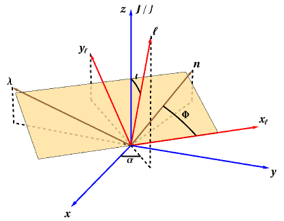
Extending previously obtained results Blanchet et al. (2011), we investigated the precessional effects by formally truncating the dynamics to the linear-in-spin order, and obtained a solution valid at any PN order when the radiation reaction is neglected. Defining the Euler angles $\iota$ and $\alpha$ as in Fig. 1, we found that the spin vectors obey (for $A=1,2$):

$$\bm{S}_{A}\cdot\bm{\ell}=\mathrm{cte}\,,\quad\bm{S}_{A}\cdot(\bm{n}+\mathrm{i}\bm{\lambda})=S^{A}_{\perp}e^{-\mathrm{i}\left((\omega-\Omega_{A})(t-t_{0})+\psi^{A}_{0}\right)}\,,$$ (10)

with $t_{0},S^{A}_{\perp},\psi^{A}_{0}$ constants, and that precessional evolution of the moving triad $(\bm{n},\bm{\lambda},\bm{\ell})$ can be entirely expressed in terms of the quantity:

$$\sin\iota\,e^{\mathrm{i}\alpha}=-\mathrm{i}\frac{J_{+}}{|\bm{J}_{\mathrm{NS}}|}e^{\mathrm{i}\phi}+\mathcal{O}(S^{2})\,,$$ (11)

where $\phi=\omega(t-t_{0})+\phi_{0}$ is the orbital phase, and $J_{+}=\bm{J}\cdot(\bm{n}+\mathrm{i}\bm{\lambda})$ is linear in spin and has a simple time dependence obtained from (10). Thus, the structure of the integrand in (9) is:

$$e^{\mathrm{i}(m\omega+p\Omega_{1}+q\Omega_{2})t}\,,\quad\text{with}~{}m\in\mathbb{Z}~{}\text{and}~{}(p,q)\in\{-1,0,1\}\,.$$ (12)

This simple time dependence allowed a straightforward computation of the tail contributions to the radiative moments. We found that the precessional contributions cancel out when combining these moments to compute the flux, which can be deduced directly from the structure of the solution for the conservative dynamics, but they do not so in the waveform and our complete calculation will be useful for a future computation of the polarizations of the wave.

The final result for the new (3.5PN+4PN) spin-orbit contributions to the energy flux reads:

$$\delta\mathcal{F}_{\mathrm{S}}\!\! = \!\!\frac{32c^{5}}{5G}\,x^{5}\,\nu^{2}\left(\frac{x^{3/2}}{G\,m^{2}}\right)\times$$ (13)

$$\!\!\!\left\{x^{2}\left[\left(\frac{476645}{6804}+\frac{6172}{189}\nu-\frac{2810}{27}\nu^{2}\right)S_{\ell}+\left(\frac{9535}{336}+\frac{1849}{126}\nu-\frac{1501}{36}\nu^{2}\right)\frac{\delta m}{m}\Sigma_{\ell}\right]\right.$$

$$\!\!\!\left.+x^{5/2}\left[\left(-\frac{3485\pi}{96}+\frac{13879\pi}{72}\nu\right)S_{\ell}+\left(-\frac{7163\pi}{672}+\frac{130583\pi}{2016}\nu\right)\frac{\delta m}{m}\Sigma_{\ell}\right]+\mathcal{O}\left(6\right)\right\}.$$

This result can be checked by testing:

• the agreement of the test-mass limit with results form the black hole perturbation theory Tagoshi et al. (1996);

• the agreement of the multipoles obtained for one body with the ones of a boosted Kerr black hole, computed as surface integrals Blanchet et al. (2005).

IV The orbital phasing of the binary

The energy flux can be combined with the result obtained for the orbital energy (6) through the balance equation $\mathcal{F}=-\mathrm{d}E/\mathrm{d}t$, which can be rewritten as an evolution equation for the phase and solved using one of the various existing PN approximants. Table 1 gives the contribution of each post-Newtonian order to the number of cycles expected to be seen in ground-based detectors, for typical LIGO/VIRGO targets, using a “Taylor 2” approximant. A more complete study by other authors Nitz et al. (2013) has investigated the overlaps between templates built with different approximants, keeping the physical parameters fixed, including or not these new contributions, and concluded to their importance.

Table 1: Contribution of each post-Newtonian order to the number of cycles, for spin-aligned quasi-circular orbits, computed using a “Taylor 2” approximant between a frequency of $10\mathrm{Hz}$, representing the entry in the detector’s band, and a cut-off frequency arbitrarily set to $x=1/6$. The result is given for typical black hole and neutron-star masses. The parameters $\kappa_{A}$ and $\chi_{A}$ stand for the orientation of the spin and the dimensionless Kerr parameter. Notice however that the relative importance of these PN contributions is affected by the choice of the approximant for the phase evolution.

LIGO/Virgo	$1.4M_{\odot}+1.4M_{\odot}$	$10M_{\odot}+1.4M_{\odot}$	$10M_{\odot}+10M_{\odot}$
Newtonian	$15952.6$	$3558.9$	$598.8$
1PN	$439.5$	$212.4$	$59.1$
1.5PN	$-210.3+65.6\kappa_{1}\chi_{1}+65.6\kappa_{2}\chi_{2}$	$-180.9+114.0\kappa_{1}\chi_{1}+11.7\kappa_{2}\chi_{2}$	$-51.2+16.0\kappa_{1}\chi_{1}+16.0\kappa_{2}\chi_{2}$
2PN	$9.9$	$9.8$	$4.0$
2.5PN	$-11.7+9.3\kappa_{1}\chi_{1}+9.3\kappa_{2}\chi_{2}$	$-20.0+33.8\kappa_{1}\chi_{1}+2.9\kappa_{2}\chi_{2}$	$-7.1+5.7\kappa_{1}\chi_{1}+5.7\kappa_{2}\chi_{2}$
3PN	$2.6-3.2\kappa_{1}\chi_{1}-3.2\kappa_{2}\chi_{2}$	$2.3-13.2\kappa_{1}\chi_{1}-1.3\kappa_{2}\chi_{2}$	$2.2-2.6\kappa_{1}\chi_{1}-2.6\kappa_{2}\chi_{2}$
3.5PN	$-0.9+1.9\kappa_{1}\chi_{1}+1.9\kappa_{2}\chi_{2}$	$-1.8+11.1\kappa_{1}\chi_{1}+0.8\kappa_{2}\chi_{2}$	$-0.8+1.7\kappa_{1}\chi_{1}+1.7\kappa_{2}\chi_{2}$
4PN	$(\mathrm{NS})-1.5\kappa_{1}\chi_{1}-1.5\kappa_{2}\chi_{2}$	$(\mathrm{NS})-8.0\kappa_{1}\chi_{1}-0.7\kappa_{2}\chi_{2}$	$(\mathrm{NS})-1.5\kappa_{1}\chi_{1}-1.5\kappa_{2}\chi_{2}$

References

- Marsat et al. (2013) S. Marsat, A. Bohé, G. Faye, and L. Blanchet, Class.Quantum Grav. 30, 055007 (2013), arXiv:1210.4143 [gr-qc] .
- Bohé et al. (2013a) A. Bohé, S. Marsat, G. Faye, and L. Blanchet, Class.Quant.Grav. 30, 075017 (2013a), arXiv:1212.5520 [gr-qc] .
- Bohé et al. (2013b) A. Bohé, S. Marsat, and L. Blanchet, Classical and Quantum Gravity 30, 135009 (2013b), arXiv:1303.7412 [gr-qc] .
- Marsat et al. (2013) S. Marsat, A. Bohé, L. Blanchet, and A. Buonanno, ArXiv e-prints (2013), arXiv:1307.6793 [gr-qc] .
- Faye et al. (2006) G. Faye, L. Blanchet, and A. Buonanno, Phys. Rev. D 74, 104033 (2006), gr-qc/0605139 .
- Blanchet et al. (2006) L. Blanchet, A. Buonanno, and G. Faye, Phys. Rev. D 74, 104034 (2006), erratum Phys. Rev. D, 75:049903, 2007, gr-qc/0605140 .
- Hartung and Steinhoff (2011) J. Hartung and J. Steinhoff, Annalen der Physik 523, 783 (2011), arXiv:1104.3079 [gr-qc] .
- Hartung et al. (2013) J. Hartung, J. Steinhoff, and G. Schäfer, Annalen der Physik (2013).
- Blanchet (2006) L. Blanchet, Living Rev. Rel. 9, 4 (2006), gr-qc/0202016 .
- Mathisson (2010) M. Mathisson, General Relativity and Gravitation 42, 1011 (2010).
- Tulczyjew (1959) W. Tulczyjew, Acta Phys. Polon. 18, 37 (1959).
- Blanchet et al. (2004) L. Blanchet, T. Damour, and G. Esposito-Farèse, Phys. Rev. D 69, 124007 (2004), gr-qc/0311052 .
- Thorne (1980) K. Thorne, Rev. Mod. Phys. 52, 299 (1980).
- Blanchet and Damour (1986) L. Blanchet and T. Damour, Phil. Trans. Roy. Soc. Lond. A 320, 379 (1986).
- Blanchet (1998) L. Blanchet, Class. Quant. Grav. 15, 1971 (1998), gr-qc/9801101 .
- Blanchet et al. (2011) L. Blanchet, A. Buonanno, and G. Faye, Phys. Rev. D 84, 064041 (2011), arXiv:1104.5659 [gr-qc] .
- Tagoshi et al. (1996) H. Tagoshi, M. Shibata, T. Tanaka, and M. Sasaki, Phys. Rev. D 54, 1439 (1996).
- Blanchet et al. (2005) L. Blanchet, T. Damour, and B. R. Iyer, Class. Quant. Grav. 22, 155 (2005), gr-qc/0410021 .
- Nitz et al. (2013) A. H. Nitz, A. Lundgren, D. A. Brown, E. Ochsner, D. Keppel, et al., (2013), arXiv:1307.1757 [gr-qc] .
- Martín-García (2002) J. Martín-García, (2002), http://metric.iem.csic.es/Martin-Garcia/xAct/.