Using Kinematic Properties of Pre-Planetary Nebulae to Constrain Engine Paradigms

Abstract

Some combination of binary interactions and accretion plausibly conspire to produce the ubiquitous collimated outflows from planetary nebulae (PN) and their presumed pre-planetary nebulae (PPN) precursors. But which accretion engines are viable? The difficulty in observationally resolving the engines warrants the pursuit of indirect constraints. We show how kinematic outflow data for 19 PPN can be used to determine the minimum required accretion rates. We consider main sequence (MS) and white dwarf (WD) accretors and five example accretion rates inferred from published models to compare with the minima derived from outflow momentum conservation. While our primary goal is to show the method in anticipation of more data and better theoretical constraints, taking the present results at face value already rule out modes of accretion: Bondi-Hoyle Lyttleton (BHL) wind accretion and wind Roche lobe overflow (M-WRLOF, based on Mira parameters) are too feeble for all 19/19 objects for a MS accretor. For a WD accretor, BHL is ruled out for 18/19 objects and M-WRLOF for 15/19 objects. Roche lobe overflow (RLOF) from the primary at the Red Rectangle level can accommodate 7/19 objects, though RLOF modes with higher accretion rates are not yet ruled out. Accretion modes operating from within common envelope evolution can accommodate all 19 objects, if jet collimation can be maintained. Overall, sub-Eddington rates for a MS accretor are acceptable but 8/19 would require super-Eddington rates for a WD.

1 Introduction

.

Binary paradigms that involve accretion (Soker & Livio, 1994; Soker, 1996, 1997, 1998; Reyes-Ruiz & López, 1999; Blackman et al., 2001; Nordhaus & Blackman, 2006) are plausibly fundamental to producing many of the asymmetric outflows observed in planetary nebulae (PN) and pre-planetary nebulae (PPN) (Balick & Frank, 2002). Their ubiquity is statistically consistent with the frequency of binaries (De Marco & Soker, 2011; De Marco et al., 2013). The influence of the latter also need not even imply their present presence if, for example, tidal shredding is involved (Nordhaus & Blackman, 2006; Nordhaus et al., 2010).

Binaries provide a source of angular momentum and free energy to form accretion disks and such disks can in turn amplify magnetic fields that transport angular momentum locally and on large scales. The latter may manifest as bipolar jets and/or winds, If jetted PN and PPN involve such disks, then both the birth and death of stars represent simllar highly aspherical states that sandwich the more spherical life of stars on the main sequence (MS).

PPN are distinguished from PN in that the former are reflection nebulae and the latter are ionization nebulae , and it is likely that PPN transition to the latter when the central star of the primary becomes sufficiently exposed to ionize the ambient nebular gas (Kwok, 2000) . Observations of high momentum outflows from PPN (Bujarrabal et al, 2001; Sahai et al., 2008) are thus important for understanding the engines of both PPN and PN. Even with a relatively conservative allotment for uncertainties, Bujarrabal et al (2001) concluded that  80% of 28 sources detected with seemingly bipolar CO molecular outflows had scalar momenta in excess of that which could be be supplied by radiation. The kinematic requirements of PPN are more demanding than those of PN, but if PPN evolve to PN, then constraints on engine paradigms of PPN also constrain PN engines.

If binaries and accretion are important to PPN and PN, a next question is which binary accretion scenarios are viable? Candidate scenarios include various modes of accretion onto either MS or white dwarf (WD) companions, or accretion from a shredded secondary onto a primary core. But the observational difficulties of detecting binaries and accretion disks warrant indirect constraints. Outflow observations can provide constraints on the needed momentum, energy, and accretion rate. Huggins (2012) estimated the kinetic energy content of jets and tori from some PPN and found that their sum was greater than the binding energy of the envelope but less than the available energy if the primary envelope accreted onto a main sequence companion. However (despite its paper title) Huggins (2012) did not constrain the power or accretion rates. Determining the minimum required accretion rates is fundamental for assessing the viability of an engine scenario. Here we give a method for doing this and to apply it to known PPN where kinematic data are available. In the long run, the method awaits more data and theory but we find that some modes of accretion can be already be eliminated for the published data used.

In Sec. 2 we discuss how to use observed outflow momenta and mass loss rates to constrain minimum accretion rates at the engine. In Sec. 3 we discuss 5 modes of accretion for which theoretical calculations or simulations have provided an accretion rate. In Sec. 4 we discuss the published data and combine this data with the results of sections 2 and 3 to produce constraint plots. We discuss the implications of this plots with respect to ruling out some modes of accretion. We conclude in section 5.

2 Minimum required accretion rates

Regardless of the particular accretion mechanism, all jets formed from an accretion disk but have a mechanical luminosity less than that of the rate of energy supply to the engine. The latter is given by (Frank et al., 2002) $\frac{1}{2}\frac{GM_{a}\dot{M_{a}}}{R_{a}}$, where $M_{a}$ is the mass of the central accretor, $R_{a}$ is the inner radius of the disk, $G$ is the gravitational constant, and $\dot{M_{a}}$ is the accretion rate, The jet mechanical luminosity then satisfies

$$L_{mec}={1\over 2}{\dot{M}}_{\textrm{j}}v_{j,N}^{2}\leq\frac{1}{2}\frac{GM_{a}\dot{M_{a}}}{R_{a}}={1\over 2}{\dot{M}}_{\textrm{a}}v_{k}^{2}(R_{\textrm{a}}),$$ (1)

where ${\dot{M}}_{\textrm{j}}$ is the jet mass loss rate, $v_{k}(R_{\textrm{a}})=\left({GM_{a}\over R_{a}}\right)^{1/2}$ is the Keplerian speed at the inner disk radius and the ”naked” jet speed

$$v_{j,N}\equiv Qv_{k}(R_{\textrm{a}})=520{\rm km/s}\left({Q\over{\sqrt{2}}}\right)\left({M_{a}\over M_{\odot}}\right)\left({R_{a}\over R_{\odot}}\right)^{-1}$$ (2)

is the maximum speed the jet would have before slowing down from swept up material. Here $Q$ is a numerical factor typically satisfying $1<Q<5$ in jet models (Blandford & Payne, 1982; Pelletier & Pudritz, 1992; Lynden-Bell, 2003; Ferrari et al., 2009), but it can depend on the environment into which the flow propagates, the location of the Alfvén surface and whether the model describes a steady magneto-centrifugal launch or a magnetic tower. In the PPN/PN context, the jet propagates into an envelope of material, and the scales at which the jet velocities are measured for PPN are large compared to those of engine launch.

Eq. (1) and Eq. (2) imply

$$\dot{M_{a}}\geq Q^{2}\dot{M_{j}}.$$ (3)

To use Eq. (3) to constrain engine models for a given choice of $Q$, we need an expression for $\dot{M_{j}}$ in terms of observables. We first write

$${{\dot{M}}_{j}\simeq M_{j,N}/t_{\textrm{acc}}},$$ (4)

where $M_{j,N}$ is the mass ejected the naked jet without swept up material, $t_{\textrm{acc}}$ is the acceleration time scale of the jet for which an upper limit is observable (discussed later). As the observed outflow is contaminated by swept up material, inferences about ${\dot{M}}_{j}$ must account for this using momentum conservation

$$p_{j}=M_{\textrm{j,ob}}v_{\textrm{j,ob}}=M_{j,N}v_{j,N},$$ (5)

where $M_{\textrm{j,ob}}$ is the mass observed in the outflow, $v_{\textrm{j,ob}}$ is the observed jet velocity. Plugging Eq. (2) into Eq. (5) and the result into (4), Eq. (3) then gives

$$\begin{array}[]{r}{\dot{M}}_{a}\geq 10^{-4}\left({Q\over 2}\right)\left({{M}_{a}\over{M}_{\odot}}\right)^{-{1\over 2}}\left({R_{a}\over{R}_{\odot}}\right)^{1\over 2}\\ \times\left({M_{\textrm{j,ob}}\over 0.1{\dot{M}}_{\odot}}\right)\left({{v}_{\textrm{j,ob}}\over 100{\rm{km/s}}}\right)\left({{t}_{acc}\over 500{\rm yr}}\right)^{-1}.\end{array}$$ (6)

We will use Eq. (6) for both MS and WD stars. Assuming that the inner disk radius equals that of the stellar photosphere (ignoring the effect from a magnetosphere). for low mass MS stars of radius $R_{*}$, the mass radius relation is approximately (Demircan & Kahraman, 1991) $R_{a}\sim 0.99R_{*}\simeq R_{\odot}\left({M_{a}\over M_{\odot}}\right)^{0.89},$ for zero age MS and $R_{a}\sim 2R_{*}\simeq R_{\odot}\left({M_{a}\over M_{\odot}}\right)^{0.75},$ for terminal age MS. Thus the right side of Eq. (6) will only weakly decrease with increasing mass.

Eq. (6) gives lower limits on ${\dot{M}}_{a}$ that are a factor ${v_{j,N}\over v_{j,ob}}>1$, larger than that which would arise if we had followed the same procedure using energy conservation instead of Eq. (5). Thus using momentum conservation is essential to obtain the more stringent limit. In addition, bulk flow energy can be lost via radiation in the outflow or conversion of bulk to thermal energy. Nevertheless, the accretion rates are still minima since (i) they presume all of the accreted power goes into the outflow; (ii) the observed values used for $t_{\textrm{acc}}$ are generally upper limits; and (iii) assumptions and uncertainties in the interpretation of the CO lines scalar momenta are underestimates (Bujarrabal et al, 2001).

3 Theoertical Accretion Rates

3.1 Bondi-Hoyle-Littleton (BHL)

For a primary AGB wind emitter of order $1M_{\odot}$ the radius above which the flow is radiatively accelerated (via dust) to its steady wind speed is $\sim 10$AU (Sandin, 2008). For a binary with such a primary interacting with an accreting secondary located outside this radiative acceleration radius $r_{dust}$, the BHL model (Edgar, 2004; Seward & Charles, 2010) provides a good approximation to the accretion rate, namely

$$\dot{M}_{\textrm{BH}}=10^{-9}{\rm M_{\odot}/{\rm yr}}\left({\dot{M}_{w}\over 10^{-5}{\rm M_{\odot}/{\rm yr}}}\right)\left({M_{S}\over M_{P}}\right)^{2}\frac{\left(\frac{v_{\textrm{or}}/v_{w}}{0.1}\right)^{4}}{\left[1+\left({v_{\textrm{or}}\over v_{w}}\right)^{2}\right]^{\frac{3}{2}}},$$ (7)

where $\dot{M}_{w}$ is the mass loss rate of the primary star, $M_{S}$ is the mass of the secondary, $M_{P}$ is the mass of the primary, $v_{w}$ is the velocity of the primary’s wind (Seward & Charles, 2010), $v_{\textrm{or}}=\left[{M_{P}/M_{S}\over 1+M_{P}/M_{S}}{GM_{P}\over a_{\textrm{or}}}\right]^{1/2}$ is the (circular) orbit speed of the secondary for an orbital separation $a_{\textrm{or}}$ about the center of mass. For $M_{P}=1.5M_{\odot}$, $v_{w}=10$km/s, $M_{S}=1M_{\odot}$, and $a_{\textrm{or}}=10$AU, ${\dot{M}}_{\textrm{BH}}=1.1\times 10^{-6}M_{\odot}$/yr, if ${\dot{M}}_{w}=1.3\times 10^{-4}M_{\odot}$/yr. Numerical simulations of Huarte-Espinosa et al (2013), generally confirm the utility of Eq. (7).

3.2 Wind Roche-Lobe Overflow (WRLOF)

When $a_{\textrm{or}}$ is large enough such that the Roche lobe of the primary is outside of the primary’s radius but less than $r_{dust}$, the wind can fill the primary’s Roche lobe and overflow onto the secondary. This was first discussed and simulated by Mohamed & Podsiadlowski (2012) for Mira ( hearafter M-WRLOF). For ${\dot{M}}_{w}=2\times 10^{-5}M_{\odot}$/yr, $M_{P}=1M_{\odot}$, $M_{S}=0.6M_{\odot}$, $a_{\textrm{or}}=20$AU, $r_{dust}=6R_{P}=10$AU, and the Roche radius of the primary $R_{L,P}=8.5$AU, they found a M-WRLOF accretion rate of ${\dot{M}}_{\textrm{WR}}\sim 0.5{\dot{M}}_{w}\simeq 5\times 10^{-7}\;\mathrm{M_{\sun}\>yr^{-1}}$. This is $\sim 20$ times the BHL rate for this set of parameters using Eq. (7).

3.3 Common Envelope

Ricker & Taam (2008) simulated a common envelope (CE) binary evolution using $M_{P}=1.05M_{\odot}$ (with core of mass $0.36M_{\odot}$) and $M_{S}=0.6M_{\odot}$. Initially, $a_{\textrm{or}}=4.3\times 10^{12}$cm and an initial red giant primary radius of $2.3\times 10^{12}$cm. The evolution was followed for 56.7 days of simulation time ($\sim 5$ orbits) by which time $a_{\textrm{or}}$ shrunk by a factor of $7$. The average accretion rate onto the secondary over the duration of the simulation and onto the primary core were ${\dot{M}}_{\textrm{CE}}\sim 10^{-2}M_{\odot}$/yr and ${\dot{M}}_{\textrm{CE,P}}\sim 6\times 10^{-2}M_{\odot}$ respectively.

These rates are significantly greater than the Eddington accretion rates for a WD or MS star. The Edddington accretion rate is that which produces the Eddington luminosity. The latter is given by

$$L_{\textrm{ed}}=\frac{1}{2}\frac{GM_{\textrm{a}}\dot{M}_{\textrm{ed}}}{R_{\textrm{a}}}=1.23\times 10^{38}\>(M_{\textrm{a}}/M_{\sun})\;\mathrm{erg/s}$$

so that the Eddington accretion rate is

$$\dot{M}_{\textrm{ed}}=\frac{2L_{\textrm{ed}}R_{\textrm{a}}}{GM_{\textrm{a}}}=2.9\times 10^{-5}\left(R_{\textrm{a}}\over 10^{9}{\rm cm}\right)\;\mathrm{M_{\sun}\>yr^{-1}},$$ (8)

where $L_{\textrm{ed}}=1.23\times 10^{38}\>(M_{\textrm{a}}/M_{\sun})\;\mathrm{erg/s}$, where we have scaled to the radius of a WD. This Eddington rate for a WD is included as a horizontal gridline in Figure 1a and for a MS star of radius $R_{\textrm{a}}=7\times 10^{10}$cm in Figure 1b.

Note that accretion onto the primary via tidal shredding of the secondary (Nordhaus & Blackman, 2006; Nordhaus et al., 2011) of a low mass star or large planet could be super-Eddington. Similar to the case of black holes (Abramowicz et al., 1980), it may here too proceed with an optically and geometrically thick disk in which the radiative diffusion time is slow compared to the accretion time, and bipolar outflows of super-Eddington mechanical luminosity. More work for this mode of accretion around white dwarfs is thus desirable.

3.4 Red-Rectangle Roche lobe overflow (RR-RLOF)

Witt et al (2009) report on observations and detailed modeling of the Red Rectangle (RR) PPN. They found that the observational features are best explained by a jet from the companion, likely powered by accretion, interacting with the wind of the primary. Their best-fit model involves MS secondary of $0.94M_{\odot}$ accreting at ${\dot{M}}_{\textrm{RR}}\sim 2-5\times 10^{-5}M_{\odot}$/yr. The authors appeal to Roche lobe overflow, as the eccentric orbit of the secondary transits through this radius. And because their accretion rate comes from inferred disk luminosity and spectra rather than from jet kinematics, their accretion rate is understandably larger than our minimum as we shall see.

4 Accretion rate constraints

4.1 Selected Objects

Table 1 shows the 18 objects from Bujarrabal et al (2001) and 1 object from Sahai et al. (2008) which have fast bipolar outflows and for which we could extract the jet momentun $p_{j}=M_{\textrm{j,ob}}v_{\textrm{j,ob}}$ and $t_{\textrm{acc}}$ for use in Eq. (6).

Table 1: List of all the objects we used, their scalar momenta ($p_{\textrm{jet}}$) and acceleration time scales ($t_{\textrm{age}}$) used. The first object is from Sahai et al. (2008) , and the rest are from Bujarrabal et al. (2001).

Object	$p_{\textrm{j}}\mathrm{\;[g\>cm/s]}$	$t_{\textrm{acc}}{\rm or}\ t_{\textrm{ppn}}\mathrm{\;[yr]}$
IRAS 05506+2414*	$8.6\times 10^{38}$	$185$
IRAS 04296+3429*	$3.3\times 10^{37}$	$370$
CRL 618*	$8.4\times 10^{38}$	$110$
Frosty Leo	$9.0\times 10^{39}$	$500$
IRAS 17436+5003*	$6.1\times 10^{38}$	$2400$
AFGL 2343*	$2.8\times 10^{40}$	$1100$
IRC+10420*	$1.5\times 10^{40}$	$900$
IRAS 19500-1709*	$5.3\times 10^{37}$	$120$
CRL 2688*	$9.6\times 10^{38}$	$120$
NGC 7027*	$3.7\times 10^{38}$	$200$
M 2-56	$1.3\times 10^{39}$	$300$
Red Rectangle*	$1.5\times 10^{35}$	$120$
OH 231.8+4.2	$3.9\times 10^{39}$	$160$
Roberts 22*	$2.2\times 10^{38}$	$440$
HD 101584	$1.5\times 10^{39}$	$30$
He 2-113*	$4.1\times 10^{37}$	$140$
CPD-568032*	$6.1\times 10^{38}$	$140$
M 1-92	$3.0\times 10^{39}$	$100$
IRAS 21282+5050*	$5.8\times 10^{38}$	$1400$

*: Used $t_{\textrm{ppn}}$ as an upper limit for $t_{\textrm{acc}}$.

For $t_{\textrm{acc}}$ in Eq. (6), we want the jet acceleration time scale or the time scale that most of the observed jet mass is ejected via the accretion engine. This can be at most, the inferred dynamical age $t_{\textrm{ppn}}$ of the PPN. For many of the objects, an acceleration time scale distinct from $t_{\textrm{ppn}}$ is unavailable so we use $t_{\textrm{ppn}}$ as an upper limit. Since $t_{\textrm{acc}}\leq t_{\textrm{ppn}}$, use of $t_{\textrm{ppn}}$ in Eq. (6) would imply a lower limit for the momentum and thus a lower limit on the minimum required accretion rate. The objects marked with a ”*” in Table 1 are those for which $t_{\textrm{ppn}}$ was used.

4.2 Graphical representation

Using Eq. 6 and the data of Table 1, we can plot the minimum required accretion rates for each object as a function of $Q$. The results are shown as diagonal lines in Fig. 1a for a MS accretor and in Fig. 1b for a WD accretor. The key difference being that for a WD of mass $0.6M_{\odot}$ and radius $10^{9}$cm, the ratio of $(R_{a}/M_{a})^{1/2}$ in Eq. (6) is 6.5 times smaller than for a MS 1$M_{\odot}$ star of radius $R_{\odot}$.

The horizontal lines on each plot represent specific accretion rate values obtained from the models of Sec. 3. In Fig. 1a from top to bottom these lines are: ${\dot{M}}_{CE}=10^{-2}M_{\odot}$/yr from section 3.3; ${\dot{M}}_{\textrm{ED}}=2.9\times 10^{-5}M_{\odot}$/yr for a WD from Eq. (8); $\dot{M}_{\textrm{BH}}=1.1\times 10^{-6}M_{\odot}$/yr for from Sec 3.1; and ${\dot{M}}_{\textrm{WR}}=5\times 10^{-7}M_{\odot}$/yr from Sec 3.2. In Fig. 1b from top to bottom these lines are: ${\dot{M}}_{CE,S}\sim 10^{-2}M_{\odot}$/yr from section 3.3; ${\dot{M}}_{\textrm{ED}}=2\times 10^{-3}M_{\odot}$/yr for a $1M_{\odot}$ MS star from Eq. (8); ${\dot{M}}_{\textrm{RR}}=(3\times 10^{-5}M_{\odot}$/yr) from Sec. 3.4; $\dot{M}_{\textrm{BH}}=1.1\times 10^{-6}M_{\odot}$/yr for from Sec 3.; ${\dot{M}}_{\textrm{WR}}=5\times 10^{-7}M_{\odot}$/yr from Sec 3.2.

Other than the line for ${\dot{M}}_{\textrm{RR}}$ from Witt et al (2009), the horizontal lines derive from accretion calculations that depend only on the accretor mass without resolving its radius. Since $0.6\leq M_{\textrm{a}}\leq 1.05M_{\odot}$ in all cases considered, we have used most of the same horizontal lines on both plots.

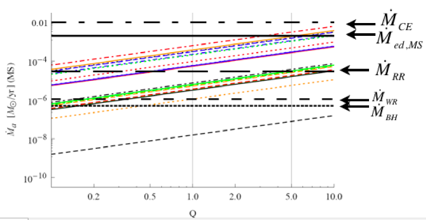
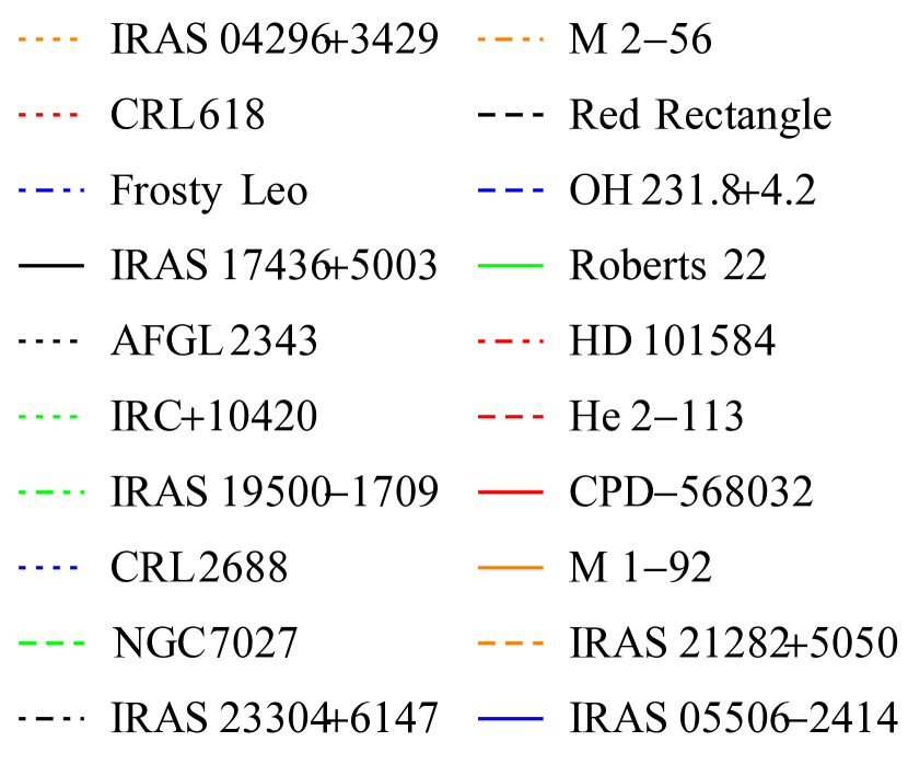
Figure 1: Mass accretion rate onto the secondary versus $Q$ from Eq. (6) for the objects of Table 1 for (a) a $0.6M_{\odot}$ WD accretor, and (b) for a $1M_{\odot}$ MS accretor. The vertical gridlines show a fiducial range of $Q$ which bounds standard theoretical jet models. The horizontal lines are indicated by the specific accretion rates discussed in Sec. 4.2. Specifically, $M_{CE}$ refers to common envelope accretion from Ricker & Taam (2008) ; ${\dot{M}}_{ed,WD}$ and ${\dot{M}}_{ed,MS}$ are the Eddington accretion rates for WD and MS stars respectively; ${\dot{M}}_{WR}$ is wind Roche lobe overflow for Mira parameters from Mohamed & Podsiadlowski (2012); ${\dot{M}}_{RR}$ is the Red Rectangle inferred Roche lobe overflow rate from Witt et al (2009); ${\dot{M}}_{BH}$ is the Bondi-Hoyle-Lyttleton rate for specific parameters given below Eq. (7).

4.3 Ruling out modes of accretion

In Fig. 1a & b, each diagonal line is a specific object. For a range of $Q$, all points on a given diagonal line above a given horizontal line correspond to the range of accretion rates which cannot be explained by the model associated with the horizontal line.

The RR is the bottom diagonal line in both Fig. 1a &b but, as discussed in Sec. 3.4, it is best modeled by the much larger Roche overflow onto a MS companion (Witt et al, 2009), shown as the ${\dot{M}}_{\textrm{RR}}$ line in Fig. (1)b. This highlights that the actual needed accretion rates can be much higher than the minima derived from outflow momenta and that other tighter constraints can obviate the need for a lower limit for a given object. We thus focus on non-RR objects.

For non-RR objects, all diagonal lines lie completely above the ${\dot{M}}_{\textrm{BH}}$ in the fiducial range of $1\leq Q\leq 5$ for the MS accretor case (Fig. 1b), ruling out BHL for this $Q$ range. For WD accretors, BHL is similarly ruled out for all non-RR objects with $1\leq Q\leq 5$ except for IRAS 04296+3429 which is ruled out for $Q>2$. For a MS star, Fig. 1b shows that ${\dot{M}}_{\textrm{WR}}$ is also ruled out for all non-RR objects For the WD case of Fig. 1a, ${\dot{M}}_{\textrm{WR}}$ is acceptable for IRAS 04296+3429 for $1\leq Q\leq 5$ and three other objects for $1\leq Q<2$ but ruled out for all others. Fig. 1b also shows that the RR-RLOF value ${\dot{M}}_{RR}$ can accommodate 7/19 objects. A mode of RLOF accretion with accretion rate significantly larger than that of RR-RLOF is not ruled out and could accommodate more objects.

Only the ${\dot{M}}_{\textrm{CE}}$ line lies above the diagonal curves for all 19 objects in both plots. Sub-Eddington rates for a MS accretor (Fig. 1b) would be acceptable for all objects in most of the range of $1\leq Q<5$, but 8/19 would require super-Eddington rates for a WD (Fig. 1a) over most of this range. Soker (2004) points out that for CE accretion modes that involve a shredded companion accreting onto a primary core, a collimated jet may more easily bore through the envelope than for the case in which the an orbiting accretor within the CE is accreting from the envelope (as in Ricker & Taam (2008)). In this respect, a higher-than RR-RLOF mode may be more desirable, in order to reduce envelope interference with jet collimation. More work is needed.

The extent to which the sources of Table 1 are kinematically typical awaits further comprehensive surveys. We do not yet have an observed distribution function of PPN fast outflows as a function of outflow momenta. In addition, simulations of the accretion modes discussed in Sec. 3 from which we have derived theoretical constraints are few, and presently for only a limited (albeit reasonable) parameter space of masses and binary radii. CE simulations (Ricker & Taam, 2008; Passy et al., 2012) are at a particularly nascent state. More theoretical and computational work focused on constraining accretion rates and developing scaling relations for each mechanism as a function of mass and binary radius would be highly desirable.

5 Conclusions

We have shown how observed outflow momenta can be used to constrain the viable accretion engines for bipolar outflows of PPN. This was accomplished by determining the minimum needed accretion rates for specific objects and then comparing these rates with those derived or computed from specific theoretical engine models. The main purpose was to demonstrate the method, anticipating that inclusion of more data and more theoretical model accretion rate calculations will further constrain allowed paradigms.

For the PPN sample of 19 objects, the present constraints (combined with independent constraints for the RR Witt et al (2009)) rule out BHL accretion onto a MS or WD star for all but maybe 1 object, and only if the accretor is a WD. For a MS accretor, we can also rule out M-WRLOF for all 19 objects when the accretor is a MS star, and for 15 objects when the accretor is a WD. For an MS accretor, the Red Rectangle Roche lobe overflow rate can accommodate 7/19 objects. Accretion from within CE evolution can accommodate all 19 objects. Sub-eddington rates for a MS accretor are acceptable, but 8/19 would require super-Eddington rates for a WD accretor. More work on the latter mode of accretion is desirable, both for accretion onto the primary core, or onto a CE companion. For the subset of modes of CE that involve accretion onto an orbiting companion, the jet may have a tougher time remaining collimated (Soker, 2004) compared to a higher-than Red Rectangle RLOF rate, and the latter is not ruled out.

Presently, jets in only a few percent of known PPN have been studied and the overall fraction of PPN with jets, let alone the distribution of momenta among them is not well constrained. The potentially provocative utility of the present approach helps to motivate more PPN kinematic survey data, more binary searches, and more theoretical/numerical simulation constraints on accretion rates. Scaling relations that would allow the addition of binary masses and radii as additional constraint dimensions on plots such as those of Fig. 1 will be particularly useful.

References

- Abramowicz et al. (1980) Abramowicz, M. A., Calvani, M., & Nobili, L. 1980, ApJ, 242, 772
- Balick & Frank (2002) Balick, B., & Frank, A. 2002, ARAA, 40, 439
- Blackman (2009) Blackman E. G., 2009, IAUS, 259, 35
- Blackman et al. (2001) Blackman, E. G., Frank, A., & Welch, C. 2001, ApJ, 546, 288
- Blandford & Payne (1982) Blandford, R. D., & Payne, D. G. 1982, MNRAS, 199, 883
- Bujarrabal et al (2001) Bujarrabal V. et al, 2001, A&A, 377, 868
- De Marco & Soker (2011) De Marco, O., & Soker, N., 2011, PASP, 123, 402
- De Marco et al. (2013) De Marco, O., Passy, J.-C., Frew, D. J., Moe, M., & Jacoby, G. H. 2013, MNRAS, 428, 2118
- Demircan & Kahraman (1991) Demircan, O., & Kahraman, G. 1991, ApSS., 181, 313
- Edgar (2004) Edgar, R. 2004, NAR, 48, 843
- Ferrari et al. (2009) Ferrari, A., Tzeferacos, P., & Zanni, C. 2009, ApSS, 322, 3
- Frank et al. (2002) Frank, J., King, A., & Raine, D. J. 2002, Accretion Power in Astrophysics, by Juhan Frank and Andrew King and Derek Raine, pp. 398. ISBN 0521620538. Cambridge, UK: Cambridge University Press, February 2002.,
- Huarte-Espinosa et al (2013) Huarte-Espinosa M. et al, 2013, MNRAS, 433, 295
- Huggins (2012) Huggins P. J., 2012, IAU Symposium, 283, 188
- Kwok (2000) Kwok, S. 2000, The origin and evolution of planetary nebulae / Sun Kwok. Cambridge ; New York : Cambridge University Press, 2000. (Cambridge astrophysics series ; 33),
- Lynden-Bell (2003) Lynden-Bell, D. 2003, MNRAS, 341, 1360
- Mohamed & Podsiadlowski (2012) Mohamed S., Podsiadlowski Ph., 2012, Baltic Ast., 21, 88
- Nordhaus & Blackman (2006) Nordhaus, J., & Blackman, E. G. 2006,MNRAS, 370, 2004
- Nordhaus et al. (2010) Nordhaus, J., Spiegel, D. S., Ibgui, L., Goodman, J., & Burrows, A. 2010, MNRAS, 408, 631
- Nordhaus et al. (2011) Nordhaus, J., Wellons, S., Spiegel, D. S., Metzger, B. D., & Blackman, E. G. 2011, Proceedings of the National Academy of Science, 108, 3135
- Passy et al. (2012) Passy, J.-C., De Marco, O., Fryer, C. L., et al. 2012, ApJ, 744, 52
- Pelletier & Pudritz (1992) Pelletier, G., & Pudritz, R. E. 1992, ApJ, 394, 117
- Reyes-Ruiz & López (1999) Reyes-Ruiz, M., & López, J. A. 1999, ApJ, 524, 952
- Ricker & Taam (2012) Ricker P. M., Taam R. E., 2012, ApJ, 746, 74
- Ricker & Taam (2008) Ricker P. M., Taam R. E., 2008, ApJ, 672, L41
- Sandin (2008) Sandin, C. 2008,MNRAS, 385, 215
- Sahai et al. (2008) Sahai, R., Claussen, M., Sánchez Contreras, C., Morris, M., & Sarkar, G. 2008, ApJ, 680, 483
- Seward & Charles (2010) Seward F., Charles P., 2010, Exploring the X-ray Universe, Cambridge University Press, 2 ed.
- Soker & Livio (1994) Soker, N., & Livio, M. 1994, ApJ, 421, 219
- Soker (1996) Soker N., 1996, ApJ, 468, 774
- Soker (1997) Soker, N. 1997, ApJS, 112, 487
- Soker (1998) Soker, N. 1998, ApJ, 496, 833
- Soker (2004) Soker N., 2004, NewA, 9, 399
- Taam & Sandquist (2000) Taam R. E., Sandquist E. L., 2000, ARA&A, 38, 113
- Witt et al (2009) Witt A. N., 2009, ApJ, 693, 1946