Classification of Human Ventricular Arrhythmia in High Dimensional Representation Spaces

Abstract

We studied classification of human ECGs labelled as normal sinus rhythm, ventricular fibrillation and ventricular tachycardia by means of support vector machines in different representation spaces, using different observation lengths. ECG waveform segments of duration 0.5-4 s, their Fourier magnitude spectra, and lower dimensional projections of Fourier magnitude spectra were used for classification. All considered representations were of much higher dimension than in published studies. Classification accuracy improved with segment duration up to 2 s, with 4 s providing little improvement.We found that it is possible to discriminate between ventricular tachycardia and ventricular fibrillation by the present approach with much shorter runs of ECG (2 s, minimum 86% sensitivity per class) than previously imagined. Ensembles of classifiers acting on 1 s segments taken over 5 s observation windows gave best results, with sensitivities of detection for all classes exceeding 93%.

I Introduction

According to the World Health Organisation data, cardiovascular disease is the leading cause of death in middle and high income countries, and among the top ten causes of death in low income countries [1]. Development of effective drug treatments that may prevent cardiac arrhythmia is therefore a high-priority challenge for modern pharmacology. For the development of such treatments it is crucial to have a clear understanding of what distinguishes different forms of arrhythmia, and based on that, establish their precise definitions. However, it is evident that although unequivocal ventricular fibrillation (VF), sustained and lethal, is incontestable in electrocardiogram (ECG) recordings, clinicians differ fundamentally about the diagnosis and appellation of transient polymorphic ventricular tachyarrhythmias, with experts in a landmark report unable to agree on whether VF, polymorphic ventricular tachycardia (VT) or torsade de pointes (TDP) best described a range of human tachyarrhythmias in a blinded test of ECG records [2]. This attests to limitations in definitions/appellation. Given that mechanisms of these tachyarrhythmias may differ [3] and responses to drugs may vary from benefit to proarrhythmia, depending on the type [4], errors in diagnosis due to unequivocal appellations are potentially hazardous. To allow preclinical research to be translatable, a definition was recently proposed to discriminate between VF, including brief and transient VF, and other polymorphic ventricular tachyarrhythmias [5]. This definition is not, however, readily transformed into an algorithm for automatic rhythm detection. Therefore, in the present study we develop novel algorithms for ventricular tachyarrhythmia classification and use them to assess whether it is possible to improve precision and accuracy of discrimination between VF and VT.

There have been many studies into the topic of differentiating sinus rhythm (SR) from VF, however fewer studies attempt to differentiate VT from VF. From a therapeutic point of view being able to differentiate between VF and VT is very important since they respond to interventions differently and VF is often lethal, while VT is often not. For VF and VT detection, Thakor et al. developed an algorithm which first applies a hard threshold to transform an ECG segment into a binary sequence, and then performs a sequential hypothesis test on the average number of zero crossings until a decision is made [6]. In [7], the authors proposed an algorithm which uses the energy distribution information in a wavelet transform domain to differentiate between VF, VT, and a VT-VF class which contains realisations that are difficult to categorise as either VT or VF. On the other hand, an estimate of the area occupied in the bispectral representation is proposed for classification between VF, VT, SR and atrial fibrillation in [8]. The standard deviations of the peak amplitudes and peak distances in a cross correlation between a window of ECG and a short window immediately prior is used to classify VT from VF in [9]. An algorithm for VF detection based on empirical mode decomposition (EMD), which creates a lower dimensional representation of ECG waveforms based on the energy in the first EMD component and its spectral entropy, was proposed in [10]. Counting the time between ECG turning points was proposed [11] to differentiate fast-VT, slow-VT and VF for use in automatic implantable cardiovertor defibrillators (AICDs). A comparison of ten methods for differentiating between non-VF and VF, for use in an automated external defibrillator (AED), was presented in [12]. The same authors subsequently proposed a phase space method [13] and demonstrate that it outperforms all methods studied in [12] in its capability to discriminate VF from non-VF segments. While all these previous works have been yielding gradual improvements, the problem of differentiating between SR, VT and VF is still not solved sufficiently accurately, the main difficulty being in differentiating between VT and VF [14]. Some of these studies even resort to creating a category specifically for the examples which are difficult to distinguish [7, 11]. Often, studies are conducted with limited or preselected data. In addition, all existing classification algorithms use heuristics to derive some low-dimensional representations of ECG signals and decision parameters, rather than provide a data-driven insight into what distinguishes one arrhythmia from another.

There is therefore a need for systematic investigation of classification of cardiac arrhythmias using representations which involve minimal information reduction, or data driven dimension reduction and classification using well established and understood statistical methods. We focus on discrimination between SR, VT, and VF, using as few heuristics as possible. In a preliminary study we considered classification in the domain of the ECG signal, and its Fourier magnitude spectra, using linear discriminant analysis (LDA), penalised discriminant analysis (PDA) and quadratic discriminant analysis (QDA), combined with principal component analysis (PCA) for data driven dimension reduction [14]. We concluded that there is benefit in considering non-linear class boundaries, but that QDA may not be the most suitable type of non-linearity, and that the training data was insufficient to obtain good generalization. In an attempt to address these issues, in the present study we considered classification with the same representation spaces using support vector machines (SVMs) [15].

One issue of interest is the selection of observation length which is most suitable for discrimination, whilst simultaneously trying to minimise detection time. In order to avoid introducing low-dimensional heuristic features, classification is performed directly in the space of ECG waveforms, and their Fourier magnitude spectra. Further, lower-dimensional representations obtained by projecting magnitude spectra onto respective principal component (PC) subspaces are also considered, in order to facilitate learning of non-linear boundaries using relatively limited training data. Even with this dimension reduction, the lowest representation dimension considered in this study is $10$, which is significantly higher dimension than features vectors used in prior art. Experimental results reported in Section IV demonstrate the benefits of considering such higher-dimensional representations for classification purposes.

The paper is organised as follows. In Section II we review a reference prior work, provide rationale for shorter observation windows, and specify dimension-reduction methods used. Section III provides details of the SVM classification framework used. Experimental procedure and results are reported in Section IV. Section V summarises the paper and draws conclusions.

II General Considerations

Given an ECG segment

$${\mathbf{x}}=\{x[n],n_{1}\leq n\leq n_{2}\}~{},$$

it is desired to be able to label it as being SR, VT or VF. For comparison, in this paper the phase space feature representation proposed in [13] is considered, since the authors conducted a thorough investigation and demonstrated its superior performance in terms of accuracy and numerical complexity compared to previously published algorithms.

II-A Reference prior art

The phase space algorithm (PSA) [13] aims at diagnosing whether a defibrillation shock should be delivered, which amounts to classifying ECG segments as VF or non-VF. The phase representation is formed by taking discretised values of samples of ${\mathbf{x}}$ as pairs $(x_{1}[n],x_{2}[n])$ in $\mathbb{R}^{2}$, where

$$x_{1}[n] = x[n]$$

$$x_{2}[n] = x[n-k]$$

while $k$ is selected to correspond to $0.5$ s. The discretisation step is chosen such that the complete range of $x_{1}[n]$ and $x_{2}[n]$ each take up to $40$ unique values. The number $N({\mathbf{x}})$ of visited boxes in this phase space is then found, and finally, the ratio

$$\eta({\mathbf{x}})=\frac{N({\mathbf{x}})}{N_{\rm max}}$$

between the number of visited boxes and the total number of boxes $N_{\rm max}=40\times 40$ is compared to an empirically determined threshold $\eta_{\rm thresh}=0.15$. If this threshold is exceeded, VF is decided, otherwise non-VF is decided. The representation space formed by $N({\mathbf{x}})$ (one-dimensional space) is referred to as PSA. We introduce a modification where the phase space is formed by pairs

$$x_{1}[n] = x[n]$$

$$x_{2}[n] = x[n]-x[n-1]$$

again discretised so that each take up to $40$ unique values. This corresponds to the standard notion of a phase space, and it may be more robust to variations in heart rate. This modification is referred to as phase space modified (PSM). In Section IV results are reported for both versions of the phase space representation in comparison to other representations introduced here.

II-B Observation length

One of the important issues that needs to be investigated is the appropriate observation length for reliable classification of cardiac arrhythmias. Longer windows contain more information, and that should lead to higher classification accuracy, up to a point beyond which increasing observation length does not provide any additional discriminating information. This plateau can be expected to be followed by a decline in classification accuracy when windows are long enough to include transitions between ECG classes. For fast and reliable diagnosis it is of interest to simultaneously minimise observation length and maximise classification accuracy. However, a systematic investigation of this issue is lacking in prior studies.

The phase space method in its original formulation [13] counts the number of visited boxes over $8$ s segments of ECG signals. Several other studies also form their respective feature vectors using $8$ s observations [12], $6$ s observations [9], or over $5$ s observations [6]. Physiological considerations, on the other hand, suggest that shorter ECG segments should suffice. According to [16], VT is considered to occur if $4$ or more consecutive QRS complexes precede their corresponding P-wave, independent of the rate. Assuming a heart rate of $60$ beats per minute or higher in humans, a $2$ s window should be sufficient to capture $2$ normal beats. Thus, at least $3$ premature QRS complexes would occur in the same $2$ s interval, and since VT is usually accompanied by an increased heart rate, quite often $2$ s should also be sufficient to capture $4$ or more premature QRS complexes. For VF, QRS complexes are no longer discernible [16], which suggests the rate of cardiac deflections (not heart rate, since the notion is not applicable) is even higher than that of VT. Therefore, a $2$ s window should be sufficient for capturing the disorder of VF also. Hence, this study will be centred around $2$ s windows, while $0.5$ s, $1$ s, and $4$ s windows will be also considered in order to assess effects of observation length on the classification accuracy and draw some conclusions on its optimal value.

II-C Dimension reduction

In order to avoid any bias due to preconceptions on what features are relevant for arrhythmia classification, classification directly in the domain of ECG waveforms is considered as a starting point. Further, Fourier magnitude spectra of ECG segments are considered as they provide representations invariant to time shifts while preserving most of the information contained in the original waveforms. At $100$ Hz sampling, which is close to the minimal sampling frequency which does not cause apparent distortions of ECG signals, $4$ s observation length results in $400$-dimensional feature space (or $200$-dimensional space if magnitude spectra are considered), which can make statistical inference challenging. This is dealt with by employing data-driven dimension reduction based on PCA. We performed PCA on magnitude spectra of each individual class, and formed sets of basis vectors by the union of top $N$ principal components from each class. Since at least 5 principal components are required to capture at least $60\%$ of the energy for each class, this is the lower limit considered. For the two class case, this forms a space of dimension $10$, and $15$ in the three-class case. The upper limit on the number of principal directions considered is $15$, since already then the dimension of the complete representation for three-class tasks becomes as high a $45$, which exceeds the dimension of $0.5$ s magnitude spectra. Since class labels are utilised, this step is performed as a supervised step in experiments reported in IV, only having access to the training set for the purposes of learning the basis vectors.

III Classification using support vector machines

Given a set of training data $\left({\mathbf{x}}_{1},\dotsc,{\mathbf{x}}_{p}\right)$ with corresponding class labels $\left(y_{1},\dotsc,y_{p}\right),~{}y_{i}\in\{+1,-1\}$, an SVM attempts to find a decision surface which jointly maximizes the margin between the two classes and minimizes the misclassification error on the training set. When the classes are linearly separable, these surfaces are linear and have the form

$$f(\mathbf{x})=\sum_{i}a_{i}y_{i}\langle{\mathbf{x}},{\mathbf{x}}_{i}\rangle+b=0,~{}a_{i}\in\mathbb{R}^{+}$$ (1)

where $\langle\cdot,\cdot\rangle$ is the inner product in $\mathbb{R}^{n}$, while the Lagrange multipliers $a_{i}$ and the bias $b$ are optimized by the training algorithm. Non-linear separators between two classes are created by means of non-linear kernel functions $K(\cdot,\cdot)$. These functions compute inner products in higher dimensional spaces, without explicitly performing the mapping, where the data could potentially be linearly separable. Analogously to the linearly separable case, the decision surface is constructed according to

$$f(\mathbf{x})=\sum_{i}a_{i}y_{i}K(\mathbf{x},\mathbf{x}_{i})+b=0$$ (2)

and the class label of a test vector ${\mathbf{x}}$ is predicted to be the sign of the score function evaluated at ${\mathbf{x}}$, i.e.

$$C({\mathbf{x}})=\mathop{\rm sgn}(f({\mathbf{x}}))~{}.$$

One commonly used kernel function is the polynomial kernel, of the form

$$K_{p}(x,y)=(1+c\langle x,y\rangle)^{d},d\in\mathbb{N}$$ (3)

where $c$ and $d$ are optimised using a grid search. Another kernel function is the radial basis function (RBF) kernel given by

$$K_{r}(x,y)=e^{-\gamma\lvert\lvert x-y\rvert\rvert^{2}},\gamma\in\mathbb{R}^{+}$$ (4)

where $\gamma$ is also optimised using a grid search.

III-A Optimising SVM parameters

Unlike with LDA and QDA, there are SVM parameters that need to be chosen optimally for best results. The idea is to avoid selecting parameters too finely tuned to the training data, while still giving good classification performance on unseen examples (test data). For SVMs using either the linear, polynomial, or RBF kernels, these parameters are:

$\mathcal{C}$: Trade-off between margin width and misclassified examples from the training data

$\gamma$: RBF kernel parameter which controls the width of the Gaussian function. Small values of $\gamma$ lead to increasing flexibility of the decision boundary, while large values of $\gamma$ lead to decreases in flexibility.

$c,d$: Polynomial kernel parameters which when increased, increase the flexibility of the decision boundary, and when small, decrease the flexibility of the decision boundary

When performing the grid search, a grid with a coarse granularity is selected with two benefits: It reduces training time required and it prevents parameters being tuned too exactly to the training data. A commonly used strategy for selecting $\mathcal{C}$ is to search a logarithmic grid, e.g. $\mathcal{C}\in\{10^{-N},10^{-N+1},\dotsc,10^{N}\}$ [17, 18]. We selected a smaller set of this range to search, depending on the kernel. For the linear kernel $\mathcal{C}$ was varied through $\frac{10^{N}}{\mathit{D}_{mean}}$, $N\in\{0,\dotsc,4\}$, where $\mathit{D}_{mean}$ is the mean Euclidean distance between training points from different classes. For the polynomial and RBF kernels, $\mathcal{C}$ was varied over $\{10^{0},\dotsc,10^{4}\}$.

The RBF kernel parameter $\gamma$ was selected such that a learned decision boundary is neither too flexible nor insufficiently flexible. An estimate for the center of a search region is given as

$70\%$	$30\%$
Tr	V	CV	CV	CV	CV	CV
$33\%$		$67\%$

Figure 1: The data is partitioned into three groups; training, validation, and CV folds. After user selected parameters are estimated with sets Tr and V, these sets are discarded, and 5-fold cross validation is performed with the sets labelled CV

$$\gamma_{start}=-\log_{10}\mathit{D}_{mean}~{}.$$ (5)

Then, with center point specified by (5), the search region is selected as

$$\gamma_{search}=10^{N},N\in[\gamma_{start}-2,\gamma_{start}+2]~{}.$$ (6)

The polynomial kernel parameters $c$ and $d$ were again chosen to enable sufficient flexibility. For this purpose, we chose $d~{}\in~{}[2,6]$, allowing increasing flexibility with polynomial degree. In order to limit the magnitude of the response of the polynomial kernel, we used the following estimate for the starting point of $c$;

$$c_{start}=\frac{1}{\displaystyle\operatorname*{arg\,max}_{k}{\lvert\lvert x_{i}\rvert\rvert^{2}}}~{},$$ (7)

where $x_{i}$ are the training data points. Then, to allow optimisation, a logarithmic range around $c_{start}$ was considered,

$$c_{search}=c_{start}\cdot 2^{2k},k\in[-3,\dotsc,3]~{}.$$ (8)

In order to ensure we have an good estimate of generalisation accuracy with limited training data, we utilise data hold out, and cross validation. For that purpose, the data was partitioned according to the scheme shown in Figure 1. For estimating user selected parameters, (e.g. the SVM cost parameter $\mathcal{C}$, RBF parameter $\gamma$, polynomial kernel parameters $c$ and $d$), one third of the data is ”held out” to be used for this estimation. Then, to estimate the generalisation accuracy, the remaining data is split into equally sized sets. One of each of the sets is held out, while the remainder is used for training a classifier (and estimating principal components, when relevant). The held out set is then used as a test set for recording classification accuracy. This is repeated with each of the sets used once as a test set. Then, the mean accuracy and standard error across all test sets can be computed. When comparing different classifiers, only the cross validation partitions are used for estimation of generalisation accuracy, even if the method did not require parameter estimation, i.e. QDA and LDA classifiers never see the data in the training and validation partitions.

III-B Multiclass classification using SVM s

For multiclass discrimination, binary SVM classifiers are combined via predefined error-correcting output code methods [19, 20]. To summarize the procedure briefly, $N$ binary classifiers are trained to distinguish between $M$ classes using a coding matrix $\textbf{W}_{M\times N}$, with elements $w_{mn}\in\{0,1,-1\}$. Classifier $n$ is trained only on data of classes $m$ for which $w_{mn}\neq 0$, with $\mathrm{sgn}(w_{mn})$ as the class label. Then, the class assignment rule is given by

$$C({\mathbf{x}})=\operatorname*{arg\,min}_{m}\sum_{n=1}^{N}\chi(w_{mn}f_{n}({\mathbf{x}}))~{},$$ (9)

where $f_{n}({\mathbf{x}})$ is the output of the $n^{\textrm{th}}$ classifier and $\chi$ is some loss function.

The error-correcting capability of a code is commensurate with the minimum Hamming distance between the rows of a coding matrix; if this minimum distance is $\delta$, then the multiclass classifier will be able to correct any $\lfloor\frac{\delta-1}{2}\rfloor$ errors [19]. For the three class problem, $\{SR,VT,VF\}$, we consider all one-vs-one (pairwise) and all one-vs-all binary classifiers, which makes a total of six binary classifiers. Note that in the case of three classes, this exhausts all possible binary classifiers. The corresponding coding matrix in this case thus has the form

$$W=\left[\begin{array}[]{rrrrrr}1&1&-1&1&1&0\\ 1&-1&1&0&-1&1\\ -1&1&1&-1&0&-1\end{array}\right]~{}.$$ (10)

A number of loss functions were compared, including hinge: $\chi(z)=\max(1-z,0)$, Hamming: $\chi(z)=[1-{\rm sgn}(z)]/2$, exponential: $\chi(z)=e^{-z},$ and linear: $\chi(z)=-z$. The hinge loss function performed best and therefore is the only loss function for which results are reported in Section IV-B. Even so, the differences of decoding with varying loss functions only changed by few percent, with exponential loss typically performing the worst, and linear loss performing almost as well as hinge loss.

III-C Classifier ensembles

Ensembles or committees of classifiers can often be combined to improve classification accuracy [18]. For that purpose we considered ensembles of decision values of binary SVM classifiers applied to ECG segments of a given length, taken with incremental shifts with respect to each other, e.g. $2$ s segments taken over $4$ s intervals with $0.5$ s shifts to form ensembles of $5$ decision values. The mean of decision values were then used as the corresponding values of $f_{n}({\mathbf{x}})$ in the loss decoding given by (9). We also considered combining individual decision values within ensembles using median, majority vote, and maximum aggregation functions, but mean gave best results.

IV Experimental Procedure and Results

IV-A Data and preprocessing

IV-A1 Data sets

Data were taken from Physiobank [21], which maintains a large online repository of various physiological signals, including ECG signals. The databases used from Physiobank were the European ST-T Database (EDB) [22], the Creighton University Ventricular Tachyarrhythmia Database (CUDB) [23], the MIT-BIH Arrhythmia Database (MITDB) [24], the MIT-BIH Malignant Ventricular Arrhythmia Database (VFDB) [25]. Only data that were explicitly labelled as SR, VT or VF were used. Due to the fact that the databases EDB and MITDB do not contain many realisations of VT or VF, additional realisations of VT and VF are taken from VFDB, and further VF realisations from CUDB. Neither of these databases contain annotations that have been audited thoroughly, so they were only used to augment examples of ventricular arrhythmias, which are few in the other databases.

IV-A2 Preprocessing

In all these databases, $250$ Hz sampling rate is used, apart from MITDB where signals are sampled at $360$ Hz. It is considered that most of the relevant information is contained in the $40$ Hz baseband [26] and that preprocessing with a $30$ Hz low pass filter does not affect experimental results [7, 10, 13, 12]. However, based on visual inspection of low-pass filtered data it was decided that $30$ Hz cut-off frequency was too low, so $49$ Hz low-pass filtering was used, followed by downsampling to $100$ Hz. In addition to this, a $0.5$ Hz high pass filter was applied to remove wandering baseline [26]. As in our previous study [14], all ECG records were normalised so that the squared sum of each record is equal to the number of samples in the record, thus making the variance of individual time samples equal to $1$.

IV-A3 Data balancing

Using rhythm annotations, either SR, VT, or VF were extracted from these databases. The continuous sequences of the rhythms were then segmented according to window length for the experiment, and shuffled randomly. Since there were many more examples of SR, this class was randomly sub-sampled to approximately the same amount as VT and VF, each of which had a total duration of approximately $6000$ s. For several reasons, balanced sets of the three classes were used. First, it is hard to understand what the relevant class priors should be, since it is highly context dependent, and also very hard to estimate. For example, in an AICD, which is always on, the presence of normal rhythm is much higher than arrhythmia, but exactly how much higher is hard to quantify (e.g it depends on the specific patient’s predisposition to an arrhythmia, underlying causes, etc). On the other hand, an AED is meant for use in emergency situations, e.g. when a patient is unconscious or not breathing, which makes the relative exposure of such a device to ECG episodes of normal rhythm and arrhythmia considerably different, and could be uniform or even skewed towards arrhythmia. Secondly, the SVM classification framework, which is used in this study, does not support notion of priors in the formulation. Finally, balanced sets prevent falsely high classification accuracy obtained by capitalising on high number of realisations of one of the classes.

IV-B SVM classification results and comparison with QDA

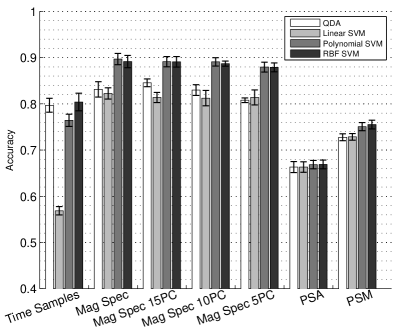
(a)

(b)

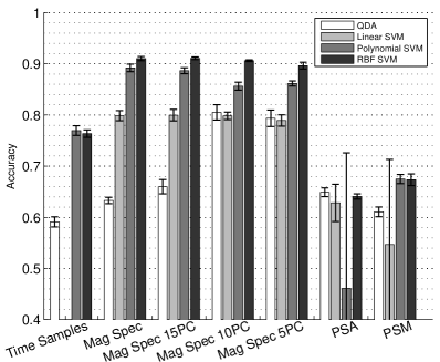
(c)

Figure 2: Average cross-validated classification accuracies with errorbars for 2 second observation length in the time, magnitude spectra, projections of magnitude spectra onto principal component spaces, PSA and PSM representation spaces. Classification is performed with linear, RBF and polynomial SVMs and compared with QDA. LABEL:sub@subfig:svm_srvt_vf non-VF versus VF. LABEL:sub@subfig:svm_vt_vf VT versus VF. LABEL:sub@subfig:svm_3way Three way classification between SR, VT and VF

Figure 3: Average cross-validated accuracies with errorbars for classification between SR, VT and VF using $0.5$, $1$, $2$ and $4$ second observation lengths in the magnitude spectra and projections of magnitude spectra onto principal component spaces. Classification is performed with RBF kernel SVM

Figure 2a, Figure 2b and Figure 2c show results of classification of non-VF vs VF, VT vs VF, and SR vs VT vs VF, respectively in the time, magnitude spectra, reduced magnitude spectra, PSA, and PSM representation spaces. This classification experiment was performed using $2$ s observation windows, as our preliminary work showed that there is minor benefit in using longer segments [14]. To assess benefits of more flexible non-linear class boundaries offered by the SVM framework, we considered SVM classification using polynomial and RBF kernels in comparison with linear kernels and QDA.

First it can be observed that classification using magnitude spectra or their reduced versions achieves much higher accuracy than classification using time-domain waveforms or PSA/PSM representations. This is in agreement with results of our preliminary analysis which used LDA and QDA classification [14]. Hence, time-domain ECG waveforms, PSA and PSM were not considered any further. In most cases at least 5% improvement in classification accuracy over QDA or linear SVM s is achieved by use of SVMs with non-linear kernel functions (Figure 2).

Corresponding sensitivity values (not included in the paper) revealed a bias in classification, usually towards SR. The average sensitivities for VT and VF did not exceed 90%, despite achieving a best accuracy of 91% with a very small standard error. The bias was more pronounced with certain classifiers (QDA) and representation spaces (time-domain ECG, phase space representations).

TABLE I: Average sensitivities for SR, VT, VF for classification of various observation lengths using RBF SVM in magnitude spectra, and reduced magnitude spectra representation spaces. Each row corresponds with a bar from Figure 3.

Window Size	Representation space	SR sens. (%)	VT sens. (%)	VF sens. (%)
0.5 seconds	Magnitude Spectra	91.8	69.8	72.0
	15PCs	91.4	70.2	71.2
	10PCs	91.4	70.2	71.2
	5PCs	92.0	69.9	71.1
1 second	Magnitude Spectra	95.3	80.4	86.2
	15PCs	95.3	80.4	86.3
	10PCs	95.4	80.1	86.1
	5PCs	95.4	79.4	84.9
2 seconds	Magnitude Spectra	97.9	86.0	89.2
	15PCs	98.2	86.2	89.0
	10PCs	97.8	85.7	88.3
	5PCs	97.9	83.5	87.6
4 seconds	Magnitude Spectra	97.0	88.0	84.9
	15PCs	96.1	85.9	85.4
	10PCs	96.9	88.8	87.7
	5PCs	96.9	87.6	88.4

Having established that the best performing representations were the magnitude spectra and their subspaces, and that SVM s with RBF kernels achieved highest accuracy, the issue of window length was revisited. Figure 3 shows results of SR versus VT versus VF classification in magnitude spectra representation spaces using SVM s with RBF kernels for observation lengths of $0.5$ s, $1$ s, $2$ s, and $4$ s. The corresponding sensitivities of individual classes are shown in TABLE I. The overall accuracy and the sensitivities improved with increasing observation lengths up to $2$ s when a performance plateau is attained, in agreement with our preliminary study in which LDA, and QDA were used [14]. The fact that increasing the segment length from $2$ s to $4$ s did not affect classification accuracy inspired forming ensembles of classifiers acting on segments taken with incremental shifts over a larger observation window.

Figure 4: Average cross-validated accuracies with errorbars for classification between SR, VT and VF using $3$, $4$, $5$ and $6$ second observation lengths in the magnitude spectra representation space with RBF SVM classifiers. Ensembles were obtained by using $2$ second or $1$ second windows, and $0.5$ second or $0.25$ second offsets.

TABLE II: Average sensitivity values for each class, SR, VT, VF shown for different window lengths, with different options for forming ensembles from the given window length. Each row corresponds with a bar from Figure 4. The representation space is magnitude spectra, and the classifier is RBF SVM.

Observation	Ensemble Options	SR sens. (%)	VT sens. (%)	VF sens. (%)
3 seconds	Window 2s / Offset 0.5s	97.7	88.8	90.5
	Window 2s / Offset 0.25s	97.9	88.9	90.3
	Window 1s / Offset 0.5s	97.4	87.2	87.7
	Window 1s / Offset 0.25s	98.3	87.3	88.0
4 seconds	Window 2s / Offset 0.5s	97.2	92.8	91.4
	Window 2s / Offset 0.25s	98.7	88.4	89.9
	Window 1s / Offset 0.5s	99.0	89.5	90.1
	Window 1s / Offset 0.25s	99.1	89.9	90.4
5 seconds	Window 2s / Offset 0.5s	98.1	90.5	92.1
	Window 2s / Offset 0.25s	98.0	90.7	92.2
	Window 1s / Offset 0.5s	98.2	93.2	93.2
	Window 1s / Offset 0.25s	98.2	93.2	92.7
6 seconds	Window 2s / Offset 0.5s	98.6	92.7	93.3
	Window 2s / Offset 0.25s	98.3	93.0	92.4
	Window 1s / Offset 0.5s	97.1	92.4	91.6
	Window 1s / Offset 0.25s	97.1	93.1	91.6

Figure 4 shows results of classification between SR, VT and VF using SVM decision values averaged over an ensemble of ECG segments, extracted from longer windows, as specified in Section III-C. These shorter segments were transformed to the best performing representation space, magnitude spectra, and classified using SVM s with RBF kernels. For this purpose $1$ s and $2$ s segments for classification were considered, taken with $0.25$ s and $0.5$ s shifts from $3$ s, $4$ s, $5$ s and $6$ s windows. For ensembles formed over $5$ s or longer, all variants performed with 90% or greater sensitivity for all classes (TABLE II). The best performing ensemble was obtained with $1$ s segments, shifted by $0.5$ s, extracted from larger windows of $5$ s. Average sensitivities obtained with these ensembles were above 93% for all classes. For these parameters, we show in Figure 5 some examples of misclassified data. Figure 5a shows three examples of rhythms labelled as VT by the databases, and classified as VF by the classifier; Figure 5b shows three examples of rhythms labelled as VF by the databases, and classified as VT by the classifier. In our opinion, these examples are classified correctly by the algorithm and mislabelled in the databases. Thus, the databases themselves impose a limitation on the best achievable accuracy, but also limit what is learnable from the data, particularly if considerable amounts of data are mislabelled.

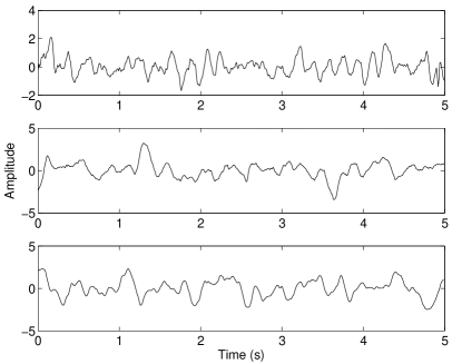
(a)

(b)

Figure 5: Examples of “misclassifications” by the best classifier from Figure 4. LABEL:sub@subfig:vt_gold_standard rhythms labeled as VT, that were classified as VF. LABEL:sub@subfig:vf_gold_standard rhythms labeled as VF, that were classified as VT.

V Conclusion

A systematic study of ECG rhythm classification was presented, to develop methods for accurate classification between SR, VT and VF. Classification was performed in the space of ECG waveforms, their magnitude spectra, and lower-dimensional approximations of magnitude spectra using projections onto their principal component spaces. All representation spaces are of much higher dimension than considered in previous studies. We found that classification accuracy improves with observation length up to about $2$ s, where it reaches a plateau, which is significantly shorter than used in previous studies [12, 13, 9]. Since VF can be highly transient in some animal models this may assist translational research.

Among considered representation spaces and classification methods, magnitude spectra and SVM classifiers with RBF kernels achieved highest accuracy. In combination they achieved classification accuracy of 91% and sensitivity of at least 86% for each class using only 2 s segments of ECG signals. However, ensembles of SVM classifiers applied to $1$ s segments over a $5$ s intervals reduced classifier bias and achieved 94% classification accuracy, with sensitivity for each class at 93% or higher.

References

- [1] W. H. Organization, “Who — the top 10 causes of death,” http://www.who.int/mediacentre/factsheets/fs310/en/index.html, 2012, [Online; accessed 8-November-2012].
- [2] R. Clayton, A. Murray, P. Higham, and R. Campbell, “Self-terminating ventricular tachyarrhythmias - a diagnostic dilemma?” The Lancet, vol. 341, no. 8837, pp. 93–95, 1993.
- [3] H. Clements-Jewery, D. Hearse, and M. Curtis, “Phase 2 ventricular arrhythmias in acute myocardial infarction: a neglected target for therapeutic antiarrhythmic drug development and for safety pharmacology evaluation,” Br. J. Pharmacol., vol. 145, no. 5, pp. 551–564, Jul 2005.
- [4] M. Chang, E. de Lange, G. Calmettes, A. Garfinkel, Z. Qu, and J. Weiss, “Pro- and antiarrhythmic effects of ATP-sensitive potassium current activation on reentry during early afterdepolarization-mediated arrhythmias,” Heart Rhythm, vol. 10, no. 4, pp. 575–582, Apr 2013.
- [5] M. J. Curtis, J. C. Hancox, A. Farkas, C. L. Wainwright, C. L. Stables, D. A. Saint, H. Clements-Jewery, P. D. Lambiase, G. E. Billman, M. J. Janse, M. K. Pugsley, G. A. Ng, D. M. Roden, A. J. Camm, and M. J. Walker, “The lambeth conventions (ii): Guidelines for the study of animal and human ventricular and supraventricular arrhythmias,” Pharmacology & Therapeutics, vol. 139, no. 2, pp. 213–248, 2013.
- [6] N. Thakor, Y.-S. Zhu, and K.-Y. Pan, “Ventricular tachycardia and fibrillation detection by a sequential hypothesis testing algorithm,” IEEE Transactions on Biomedical Engineering, vol. 37, no. 9, pp. 837–843, September 1990.
- [7] K. Balasundaram, S. Masse, K. Nair, T. Farid, K. Nanthakumar, and K. Umapathy, “Wavelet-based features for characterizing ventricular arrhythmias in optimizing treatment options,” in Annual International Conference of the IEEE Engineering in Medicine and Biology Society, September 2011, pp. 969–972.
- [8] L. Khadra, A. Al-Fahoum, and S. Binajjaj, “A quantitative analysis approach for cardiac arrhythmia classification using higher order spectral techniques,” IEEE Transactions on Biomedical Engineering, vol. 52, no. 11, pp. 1840–1845, November 2005.
- [9] J. Ruiz, E. Aramendi, S. Ruiz de Gauna, A. Lazkano, L. Leturiondo, and J. Gutierrez, “Distinction of ventricular fibrillation and ventricular tachycardia using cross correlation,” in Computers in Cardiology, September 2003, pp. 729–732.
- [10] B. Bai and Y. Wang, “Ventricular fibrillation detection based on empirical mode decomposition,” in 5th International Conference on Bioinformatics and Biomedical Engineering, May 2011, pp. 1–4.
- [11] W. Olson, D. Peterson, L. Ruetz, B. Gunderson, and M. Fang-Yen, “Discrimination of fast ventricular tachycardia from ventricular fibrillation and slow ventricular tachycardia for an implantable pacer-cardioverter-defibrillator,” in Computers in Cardiology, September 1993, pp. 835–838.
- [12] A. Amann, R. Tratnig, and K. Unterkofler, “Reliability of old and new ventricular fibrillation detection algorithms for automated external defibrillators,” BioMedical Engineering OnLine, vol. 4, no. 1, p. 60, 2005.
- [13] ——, “Detecting ventricular fibrillation by time-delay methods,” IEEE Transactions on Biomedical Engineering, vol. 54, no. 1, pp. 174–177, Jan 2007.
- [14] Y. Alwan, Z. Cvetković, and M. J. Curtis, “High-dimensional discriminant analysis of human cardiac arrhythmias,” in Proceedings European Signal Processing Conference, 2013, In press.
- [15] C. Cortes and V. Vapnik, “Support-vector networks,” in Machine Learning, 1995, pp. 273–297.
- [16] M. J. A. Walker, M. J. Curtis, D. J. Hearse, R. W. F. Campbell, M. J. Janse, D. M. Yellon, S. M. Cobbe, S. J. Coker, J. B. Harness, D. W. G. Harron, A. J. Higgins, D. G. Julian, M. J. Lab, A. S. Manning, B. J. Northover, J. R. Parratt, R. A. Riemersma, E. Riva, D. C. Russell, D. J. Sheridan, E. Winslow, and B. Woodward, “The lambeth conventions: guidelines for the study of arrhythmias in ischaemia, infarction, and reperfusion,” Cardiovascular Research, vol. 22, no. 7, pp. 447–455, 1988.
- [17] J. Shawe-Taylor and N. Cristianini, Kernel Methods for Pattern Analysis. New York, NY, USA: Cambridge University Press, 2004.
- [18] T. Hastie and R. Tibshirani, The Elements of Statistical Learning: Data Mining, Inference, and Prediction, 2nd ed., ser. Springer Series in Statistics. Springer, 2009.
- [19] T. G. Dietterich and G. Bakiri, “Solving multiclass learning problems via error-correcting output codes,” Journal of Artificial Intelligence Research, vol. 2, pp. 263–286, 1995.
- [20] E. L. Allwein, R. E. Schapire, and Y. Singer, “Reducing multiclass to binary: a unifying approach for margin classifiers,” Journal of Machine Learning Research, vol. 1, pp. 113–141, 2001.
- [21] A. L. Goldberger, L. A. N. Amaral, L. Glass, J. M. Hausdorff, P. C. Ivanov, R. G. Mark, J. E. Mietus, G. B. Moody, C.-K. Peng, and H. E. Stanley, “Physiobank, physiotoolkit, and physionet : Components of a new research resource for complex physiologic signals,” Circulation, vol. 101, no. 23, pp. e215–e220, 2000.
- [22] A. Taddei, G. Distante, M. Emdin, P. Pisani, G. B. Moody, C. Zeelenberg, and C. Marchesi, “The european st-t database: standard for evaluating systems for the analysis of st-t changes in ambulatory electrocardiography,” European Heart Journal, vol. 13, no. 9, pp. 1164–1172, 1992.
- [23] F. Nolle, F. Badura, J. Catlett, R. Bowser, and M. Sketch, “Crei-gard, a new concept in computerized arrhythmia monitoring systems,” Computers in Cardiology, vol. 13, pp. 515–518, 1986.
- [24] G. Moody and R. Mark, “The impact of the mit-bih arrhythmia database,” Engineering in Medicine and Biology Magazine, IEEE, vol. 20, no. 3, pp. 45–50, June 2001.
- [25] S. Greenwald, “Development and analysis of a ventricular fibrillation detector,” Master’s thesis, MIT Dept. of Electrical Engineering and Computer Science, 1986.
- [26] B. Raghavendra, D. Bera, A. Bopardikar, and R. Narayanan, “Cardiac arrhythmia detection using dynamic time warping of ecg beats in e-healthcare systems,” in IEEE International Symposium on a World of Wireless, Mobile and Multimedia Networks, June 2011, pp. 1–6.