Exciton coupling induces vibronic hyperchromism in light-harvesting complexes

Abstract

The recently suggested possibility that weak vibronic transitions can be excitonically enhanced in light-harvesting complexes is studied in detail. A vibronic exciton dimer model which includes ground state vibrations is investigated using multi-configuration time-dependent Hartree method with a parameter set typical to photosynthetic light-harvesting complexes. Absorption spectra are discussed in dependence on the Coulomb coupling, the detuning of site energies, and the number of vibrational mode. Calculations of the fluorescence spectra show that the spectral densities obtained from the low temperature fluorescence line narrowing measurements of light-harvesting systems need to be corrected for the exciton effects. For the J-aggregate configuration, as in most of the light-harvesting complexes, the true spectral density has larger amplitude than what is obtained from the measurement.

1 Introduction

In photosynthesis light absorption and charge separation take place in specialised multi-chromophoric systems. While the reaction centre (RC) complexes, where the primary charge separation occurs, are very similar in different photosynthetic systems, the light-harvesting antennas show a wide variety [1]. Clearly, it is possible to optimise absorption of light and make excitation transport to RC efficient in many different ways. One of the strategies used in most of the photosynthetic systems is to organise the pigments energetically in an energy funnel with the RC in the bottom of the sink [2]. In addition, the pigment molecules are usually close enough to enable sufficient resonant interaction and thereby fast excitation transport. Such general optimisation strategies are widely reported and well understood in photosynthetic antenna systems.

A result of the relatively dense packing of the pigment molecules in the antenna complexes is the emergence of delocalised Frenkel exciton states [3, 4, 5, 6]. The later has led to recognition of the role of memory effects and coherence in Frenkel exciton dynamics in photosynthetic light-harvesting. The discussion was recently revitalised by novel coherent multidimensional spectroscopy measurements revealing long-lived oscillatory features in a so called Fenna-Mathews-Olson (FMO) light-harvesting antenna complex [7]. The oscillations were interpreted as electronic coherences and their long lifetime was taken as an evidence for possible coherent excitation transport. It was argued that parallel coherent excitation transport pathways may enable interference-based quantum optimisation possibilities for making excitation transfer through the FMO complexes more efficient. Analogous observations were also reported for light-harvesting complexes in photosynthetic marine algae [8]. This initiated numerous new theoretical investigations of the role of coherence in excitation energy transport [9, 10, 11]. An important conclusion drawn from these efforts concerned the optimal parameter region of the transport - it was realized that the most efficient transport takes place in the intermediate regime between fully coherent and incoherent transport where the inter-pigment resonance interaction and the system-bath interaction are not so different [12, 13]. Interestingly, the efficiency curve has a rather flat maximum meaning that optimal transport can be achieved by quite a broad set of parameters.

In contrast to the large number of simulations following the excitation dynamics [10, 14, 15, 16, 17], much fewer studies have made the effort to calculate the coherent multidimensional spectroscopy signals, which would directly correspond to what is observed in experiment [18, 19, 20]. It turned out that reproducing the long-lived oscillations in calculated 2D spectra as electronic coherences is not straightforward. Even studies based on hierarchy equations of motion (HEOM) where bath memory effects are included formally exact could not reach agreement with experimental observations [21, 22]. Additional assumptions had to be made. For example, assuming correlated static and dynamic disorder at different pigment sites led to long-lived electronic coherences [23, 24]. However, neither correlated nuclear motions nor inhomogeneous broadening has any independent support. Quite the opposite. Thorough molecular dynamics studies did not show any evidence for such correlations [25]. A recent study using HEOM approach produced long-lasting electronic coherences [26]. The authors used a spectral density, which fitted well the fluorescence line narrowing experiments [27] for frequencies above 50 cm^-1. However, the low-frequency region, which is particularly important for electronic dephasing and is most sensitive to temperature, had an unrealistically small amplitude.

Initially, the possible vibrational origin of the oscillatory features in the two-dimensional (2D) signal in FMO was discarded since the nuclear modes in the frequency region of observed oscillations ($\sim$150 cm^-1) are very weakly coupled to the electronic transition leading to a negligible Huang-Rhys factor $S$. In the 180 cm^-1 region there are a few modes with the total $S$ reaching almost 0.05 [27, 28], but even this is too weak to produce significant oscillatory features in 2D signals. Transition energies of the bacteriochlorophyll (BChl) molecules in FMO are quite well established [29]. It turns out that the 0-1 vibronic transition energy of the 180 cm^-1 mode region on the red-most BChl is almost in resonance with the 0-0 transition energy of one of its neighbours. Consequences of such resonance for natural light-harvesting have not been fully analysed before. A vibronic exciton model where one mode per pigment is treated explicitly [30] was applied for calculating electronic 2D response functions of FMO [31]. It was shown that owing to the resonance, the weak transition of mainly vibronic origin at the lowest energy BChl obtains a significant additional oscillator strength due to mixing with the strong purely electronic transition at the neighbouring molecule. Furthermore, the long-lived oscillations observed in 2D experiments were explained by the fact that energy fluctuations of the vibrational levels of a molecule are correlated and consequently the corresponding coherences between vibronic levels have a long lifetime. The intensity borrowing is quite robust and moving to some extent out from the resonance due to the inhomogeneous broadening does not influence the results appreciably.

An analogous resonance between 0-0 and 0-1 transitions of neighbouring pigments was recently used in an excitonic dimer model where adiabatic potential energy surfaces were calculated [32, 33]. The authors argue that because of the near resonance between the levels, the adiabatic approximation breaks down and non-adiabatic coupling has to be taken into account. The non-adiabatic coupling causes mixing of the states leading to intensity redistribution very much like in Ref. [31]. Excitation dynamics due to the non-adiabatic coupling in the context of light-harvesting complexes has been analysed in terms of curve-crossing and surface hopping [34, 35]. Schröter and Kühn studied the interplay between non-adiabatic dynamics and Frenkel exciton transfer in aggregates where both S₁ and S₂ transitions were considered [36]. Also excitation annihilation has been described as non-adiabatic coupling between one- and two-exciton manifolds [37, 38]. Tiwari et al. [32] investigated a different situation where the potentials are nested and the crossing points are very far from the equilibrium resembling the situation in internal conversion. Using 2D signal calculations the authors argue that the long-lived oscillating features of 2D spectroscopy of light-harvesting systems could be explained in terms of ground state coherent nuclear motions excited via enhanced transitions with strong vibronic character.

Several other studies have recently addressed the issue how to separate the electronic and vibrational quantum beats in electronic 2D spectroscopy. Comparison of the oscillatory patterns and oscillation phases in two representative systems, displaced oscillator and excitonic dimer, was reported [39]. The model was further developed for a dimer with ground state vibrational levels included [40]. The ground and excited state vibrational coherences were thoroughly compared in vibronic exciton dimer model [41]. Oscillatory phonon features in colloidal quantum dots were modelled [42] and it was shown that following separately positive and negative frequency components of the population time Fourier transform gives additional control over the Liouville pathways thereby enabling a more clear distinction between electronic and vibrational beatings [43].

We point out that the method used by Christensson et al. [31], a so called one particle approximation (OPA), only includes excited state vibrations. In order to account for the ground state vibrational states, at least the two particle approximation (TPA) [44, 45] has to be employed. TPA is exact in case of a dimer and has been used for analyses of 2D spectra [32, 40]. Various analogous approaches have been applied for modelling a vibronic dimer [46, 47]. An obvious question arrises - what effects does one miss by using simple OPA calculations as in [31] compared to the exact solution of the problem. Here we address the issue by carrying out a comparison of OPA and TPA using a model dimer resembling two neighbouring low-energy BChl molecules in the FMO. The numerically exact reference is provided by the multi-configuration time-dependent Hartree (MCTDH) method [48, 49].

The article is organised as follows. We start from presenting the basics of the the vibronic exciton model and the OPA as well as MCTDH approaches. The theory is followed by comprehensive model calculations of a vibronic heterodimer for various parameter sets. We show that despite of the dominantly monomeric character of the heterodimer, the intensities of the vibrational features in the fluorescence spectrum are significantly affected. This has consequences for how to use the fluorescence line narrowing spectroscopy to experimentally determine the spectral densities [53]. In the final part the results are discussed and conclusions formulated.

2 Theoretical Model

2.1 Frenkel Exciton Hamiltonian

In the following we will use the Frenkel exciton Hamiltonian describing coupled electronic (zero, $|0\rangle$, and one-exciton, $|m\rangle$, space) and nuclear degrees of freedom, $\mathbf{Q}=\{\mathbf{Q}_{m}\}$, [3]

$$H_{\rm agg}(\mathbf{Q}) = H^{(0)}(\mathbf{Q})+H^{(1)}(\mathbf{Q})\,,$$ (1)

$$H^{(0)}(\mathbf{Q}) = \sum_{m}H_{m,g}(\mathbf{Q}_{m})\left|0\right>\left<0\right|\equiv\mathcal{E}_{0}\left|0\right>\left<0\right|\,,$$ (2)

$$H^{(1)}(\mathbf{Q}) = \sum_{mn}[\delta_{mn}(\mathcal{E}_{0}+U_{m,e}(\mathbf{Q}_{m})+J_{mn}]|m\rangle\langle n|\,.$$ (3)

Denoting the monomeric electronic states by $\left|a_{m}\right>$ where $a=(g,e)$ are the ground and excited states, one has $\left|0\right>=\prod_{m}\left|g_{m}\right>$ and $\left|m\right>=\left|e_{m}\right>\prod_{n\neq m}\left|g_{n}\right>$. The nuclear motion will be describe in the displaced oscillator model, i.e. the ground state Hamiltonian and excited state coupling read for each site ($E_{m}$: electronic energy)

$$H_{m,g}(\mathbf{Q}_{m}) = \sum_{\xi}\frac{\hbar\omega_{\xi}}{2}\left(-\frac{\partial^{2}}{\partial Q_{m,\xi}^{2}}+Q_{m,\xi}^{2}\right)\,,$$ (4)

$$U_{m,e}(\mathbf{Q}_{m}) = E_{m}+\sum_{\xi}\hbar\omega_{\xi}g_{\xi}Q_{m,\xi}\,.$$ (5)

Here, $\omega_{\xi}$ ($\xi=1,\ldots,N_{\rm vib}$) is the vibrational frequency of mode $Q_{m,\xi}$ (note the use of dimensionless units) which is assumed to be identical for the different monomers. The same approximation is made for the linear coupling constant, $g_{\xi}$, which relates to the Huang-Rhys factor as $S_{\xi}=g_{\xi}^{2}/2$.

Absorption and emission spectra will be calculated in Condon-approximation for the monomeric transition dipole matrix elements $d_{m}$, summed to give the aggregate dipole operator according to

$$d=\sum_{m}d_{m}\left|m\right>\left<0\right|+{\rm h.c.}\,.$$ (6)

2.2 $n$-Particle Approach

The problem of coupled exciton-vibrational dynamics can be approached by a $n$-particle approximation scheme [44]. To this end we introduce vibrational states for the different potential energy surfaces according to $\left|M_{m,a}\right>$ where it is understood that $M_{m,a}$ could be a multi-index in cases where several vibrational modes per monomer need to be taken into account. The eigenstates $\left|\alpha^{(1)}\right>$ of $H^{(1)}(\mathbf{Q})$ can be expanded as

$$\left|\alpha^{(1)}\right>=\sum_{m,\mu}C_{m,\mu}(\alpha^{(1)})\left|m\mu\right>+\sum_{mn}\sum_{\mu\nu}C_{mn,\mu\nu}(\alpha^{(1)})\left|m\mu,n\nu\right>+\ldots$$ (7)

with the one-particle states

$$\left|m\mu\right>=\left|e_{m}\right>\left|\mu=M_{m,e}\right>\prod_{n\neq m}\left|g_{n}\right>\left|0_{n,g}\right>$$ (8)

and the two-particle states

$$\left|mn,\mu\nu\right>=\left|e_{m}\right>\left|\mu=M_{m,e}\right>\left|g_{n}\right>\left|\nu=N_{n,g}\right>\prod_{k\neq m,n}\left|g_{k}\right>\left|0_{k,g}\right>$$ (9)

In principle Eq. (7) will contain further terms, but for the present case of a molecular heterodimer, the two-particle ansatz is already exact. The restriction to the first term is the so-called OPA.

Using the eigenstates, Eq. (7), the absorption spectrum will be calculated in the zero temperature limit as ($I_{0}$ normalisation constant)

$$I(\omega)=I_{0}\omega\sum_{\alpha^{(1)}}\frac{\Gamma|\langle\alpha^{(1)}|d|\alpha^{(0)}=0\rangle|^{2}}{(\omega-\omega_{\alpha^{(1)}0})^{2}+\Gamma^{2}}\,,$$ (10)

where $\Gamma$ is a parameter mimicking the finite line width (dephasing time) of the real system, $|\alpha^{(0)}\rangle$ denotes the eigenstates of $H^{(0)}$ with $|\alpha^{(0)}=0\rangle$ being the overal ground state (see below), and $\omega_{\alpha^{(1)}\alpha^{(0)}}$ is the transition frequency. The emission spectrum is calculated as

$$F(\omega)=F_{0}\sum_{\alpha^{(1)},\alpha^{(0)}}P(E_{\alpha^{(1)}})\frac{\Gamma|\langle\alpha^{(1)}|d|\alpha^{(0)}\rangle|^{2}}{(\omega-\omega_{\alpha^{(1)}\alpha^{(0)}})^{2}+\Gamma^{2}}\,,$$ (11)

where $P(E_{\alpha^{(1)}})$ is the Boltzmann population of an one-exciton-vibrational state with energy $E_{\alpha^{(1)}}$ and $F_{0}$ is a normalisation constant.

2.3 MCTDH Approach

In principle the $n$-particle approach provides a systematic route to the exact eigenstates of the one-exciton Hamiltonian. However, with increasing aggregate size and number of vibrational coordinates one will soon face the dimensionality bottleneck and the problem will become numerically intractable. An efficient alternative approach is the MCTDH method, which rests on the expansion of the time-dependent state vector into a basis of time-dependent Hartree products that are composed of single particle functions (SPFs) [49, 48]. Applications to exciton dynamics and spectroscopy have been given in Refs. [50, 51].

First, the state vector is expanded in terms of the one-exciton basis, i.e

$$|\Psi({\bf Q};t)\rangle=\sum_{m}\chi_{m}({\bf Q};t)\,|m\rangle\,.$$ (12)

In a next step the nuclear wave function is written in MCTDH form as follows

$$\chi_{m}(\mathbf{Q},t)=\sum_{j_{1}\ldots j_{D}}^{{n_{j_{1}}\ldots n_{j_{D}}}}C^{(m)}_{j_{1},\ldots,j_{D}}(t)\phi^{(m)}_{j_{1}}(Q_{1};t)\ldots\phi^{(m)}_{j_{D}}(Q_{D};t)\,.$$ (13)

Here, the $C^{(m)}_{j_{1},\ldots,j_{D}}(t)$ are the time-dependent expansion coefficients weighting the contributions of the different Hartree products, which are composed of SPFs, $\phi^{(m)}_{j_{k}}(Q_{k};t)$, for the $k$th nuclear degree of freedom in state $m$. Overall there are $D=N_{\rm agg}\times N_{\rm vib}$ nuclear degrees of freedom.

Although it is in principle possible to obtain eigenstates with the MCTDH method, being a time-dependent approach, it is more suited to solve the time-dependent Schrödinger equation. Therefore we will use it to calculate the absorption spectrum according to the time-dependent reformulation of Eq. (10) [3]

$$I(\omega)=I_{0}\omega\,{\rm Re}\int_{0}^{\infty}dt\,e^{i\omega t-t/\tau}\langle\Psi_{0}|de^{-iH_{\rm agg}(\mathbf{Q})t/\hbar}d|\Psi_{0}\rangle\,,$$ (14)

where $d$ is dipole operator, Eq. (6) and $\left|\Psi_{0}\right>$ is the ground state wave function. Since there is no coupling in $H^{(0)}$, it is given as a Hartree product, i.e.

$$\left|\Psi_{0}\right>=\phi^{(0)}_{0}(Q_{1})\ldots\phi^{(0)}_{0}(Q_{D})\left|0\right>$$ (15)

with $\phi^{(0)}_{0}(Q_{j})$ being the respective ground state wave function for the $j$th mode. All wave packet propagation simulations have been performed using the Heidelberg program package [52]. The MCTDH dimer setup, which has been applied here, includes three electronic states (one ground state and two singly excited states). Since the ground state has been used for the preparation of the initial wave packet only, one SPF per mode has been sufficient to describe it properly. The actual propagation of the wave packet takes place on the two excited states; here four SPFs were necessary to obtain converged results. As a primitive basis we have used a harmonic oscillator (20 points) discrete variable representation within an interval of [-3.5:3.5] for all modes. For all calculations the multi-set method was used.

3 Results and Discussion

In the following application the case of two sites (vibronic heterodimer, $m=(D,A)$) will be considered. The parameters are chosen to mimic the situation in the FMO complex. A number of studies have proposed electronic Hamiltonian of the complex, based on modelling of a set of spectroscopic observables. For a review see [54]. There is a general agreement that the BChl 3 and 4 have the lowest site energies. The transition energy difference is proposed to be from about 110 to 180 cm^-1 . Excitonic coupling between these two molecules is negative with values from about -50 to -75 cm^-1 [29]. Fluorescence line narrowing spectroscopy has revealed that at around 180 cm^-1 there are a few vibrational modes in the FMO lowest energy BChl with a total Huang-Rhys factor 0.03 [27]. We point out that the analogous experiments with BChl in triethylamine give a somewhat higher value of 0.04 [28]. Having these parameters in mind we formulate our vibronic dimer as follows. The properties of the eigenstates and spectra of the model will be scrutinised in dependence on the Coulomb coupling $J\equiv J_{\rm DA}$ and the heterogeneity, $\Delta E\equiv E_{\rm D}-E_{\rm A}$. For reference we will use $\Delta E=180$ cm^-1 and $J_{\rm DA}/hc=-90$ cm^-1 . First, each site is coupled to one vibrational mode with parameters $\omega/2\pi c=180$ cm^-1 and $S=0.05$. In the following we will start with a discussion of the differences between exact and OPA in the absorption spectrum for transitions to the one-exciton manifold. The focus will be on the dependence on detuning between the local excitation energies and the Coulomb coupling. In order to study multi-mode effects a second model including additional vibrational modes with varying frequency and Huang-Rhys factor will be considered in an up to three-mode model ($\omega/2\pi c=365$ cm^-1 , $S=0.019$ and $\omega/2\pi c=260$ cm^-1 , $S=0.023$). The actual frequencies of the modes were chosen as approximately 1.5 and 2 times the original frequency $\omega/2\pi c=180$ cm^-1 . The corresponding Huang Rhys factors were chosen to represent the total S of the nearby modes reported in [28]. Finally, the temperature dependence is addressed in terms of the emission spectrum.

3.1 Validity of OPA

The dependence of exact and OPA absorption spectra on the Coulomb coupling $J_{\rm DA}$ ($\Delta E/\hbar\omega=1$) and the detuning $\Delta E$ ($J_{\rm DA}/\hbar\omega=-0.5$) are compared in Fig. 1. This figure also contains the respective dependencies of the bare energy levels.

First we notice that for $J_{\rm DA}=0$ the two cases show different degeneracies of energy levels due to the restricted state space of the OPA. Looking at the dependence on $J_{\rm DA}$ upon increasing its value, energy levels are shifted and degeneracies are partly lifted. Around $J_{\rm DA}/\hbar\omega\approx 0.85$ and $\approx 1.35$ energy levels approach each other showing partially avoided crossings in the exact case. This pattern is not at all reproduced by the OPA. Overall only the lowest state shows an agreement between exact and OPA calculations. The same conclusion can be drawn from the $\Delta E$ dependence shown in Fig. 1d,e.

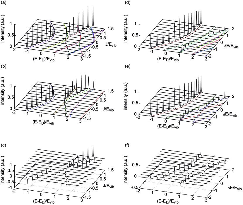
Figure 1: Absorption spectrum, Eq. (10), as function of $J=J_{\rm DA}$ for $\Delta E/\hbar\omega=1$ (left) and as function of $\Delta E$ for $J_{\rm DA}/\hbar\omega=-0.5$ (right) using exact (a,d) and OPA (b,e) approaches. Panels (c) and (f) show the respective differences. ($E_{\rm vib}=\hbar\omega$)

Comparing the rather different behaviour of the spectrum of $H^{(1)}$ for exact und OPA models, the question arises how this will reflect in absorption spectra. Here we notice from Fig. 1 that the differences between the exact and OPA are particularly large for the $J_{\rm DA}$-dependence. Of course, whether or not deviations are visible depends on distribution of oscillator strength. Therefore the positive coupling part of the $J_{\rm DA}$ dependence is more visibly influenced. As a consequence OPA gives reasonable results as far as the $\Delta E$-dependence is concerned since $J_{\rm DA}<0$ for the present model. Generally, there is a trend that despite of radically different energy level structure in the two models, when it comes to the intensities of the spectral features, the models give surprisingly similar results. If one would use broader line shapes, the resulting spectra would not be very different for most of the used parameters. Interestingly, it is not true that OPA necessarily yields a simpler spectrum as one would expect on the basis of the energy level structure of the one-exciton Hamiltonian. Indeed, one can state that the exact case shows more pronounced collective effect, i.e. oscillator strength is essentially located in a single transition.

3.2 Multi-mode Effects

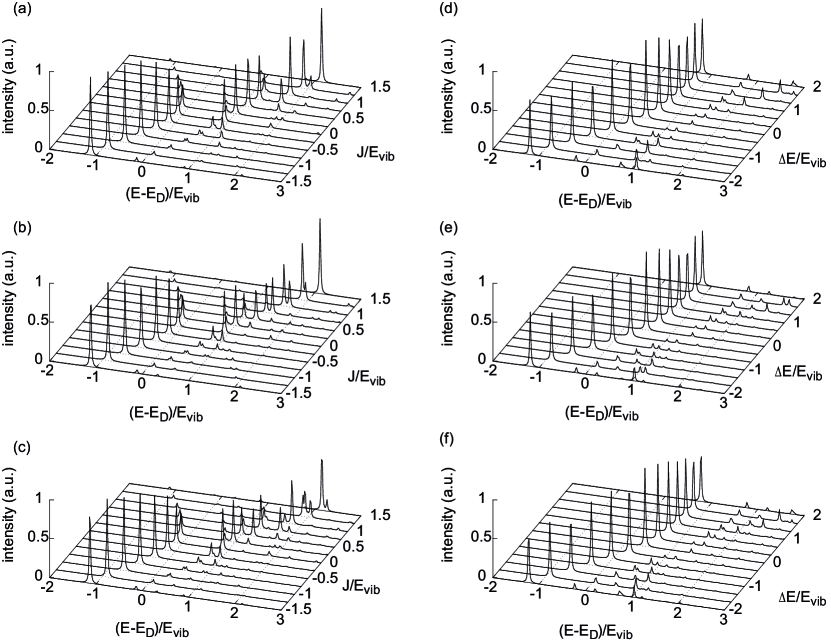
Figure 2: Absorption spectrum, Eq. (14), as function of $J=J_{\rm DA}$ for $\Delta E/\hbar\omega=1$ (left) and as function of $\Delta E$ for $J_{\rm DA}/\hbar\omega=-0.5$ (right) for two different two-mode models and a three-mode model. All results contain the mode at 180 cm^-1 used before. Additional modes: (a,d) $\omega/2\pi c=365$ cm^-1 and $S=0.019$, (b,e) $\omega/2\pi c=260$ cm^-1 and $S=0.023$, (c,f) both modes of panels (a-d). ($E_{\rm vib}=\hbar\omega$, 180 cm^-1 mode)

In the following we discuss the effect of multiple modes, coupling to the electronic transitions. Results of MCTDH simulations of absorption spectra are shown in Fig. 2. Overall one can state that since for large negative $J_{\rm DA}$ oscillator strength is concentrated in the lowest state which has dominantly electronic character, a pronounced effect of further modes is seen for positive couplings only. For the case of FMO this leads to rather similar spectra as a function of the detuning $\Delta E$ as can be seen from the right column of Fig. 2. In case of positive coupling the details of spectral changes depend, of course, on the mode parameters, but the net effect is a broadening due to the more complex structure of the exciton-vibronic states.

3.3 Temperature Dependence of Emission Spectra

Results for the emission spectrum of the one-mode model as a function of Coulomb coupling and detuning are shown in Fig. 3 for two different temperatures. Owing to the small Huang-Rhys factor the spectra at 4K essentially are showing the 0-0 transition and a small shoulder due to the 0-1 transition in Fig. 3a. The intensity of these transitions gradually drops down upon increasing $J_{\rm DA}$ in the positive domain due to H-aggregate formation. This does not occur upon increasing the detuning in panel (c) where the spectrum becomes close to that of a monomer for large $\Delta E$. For $T=300$K the spectrum is much more structured as can be seen from Fig. 3b,d. The level structure with a complex intensity pattern makes it impossible to draw a priori conclusions on the thermal occupation. Notice that due to the Coulomb coupling the spacing between the peaks above the 0-0 transition is not equal to a vibrational quantum. Since the lowest energy fluorescence feature is due to the ground state vibrational structure, it is still shifted from 0-0 by the vibrational frequency.

Figure 3: Emission spectra, Eq. (11), as function of $J=J_{\rm DA}$ for $\Delta E/\hbar\omega=1$ and $T=4$K (a) and 300 K (b) and as a function of $\Delta E$ for $J_{\rm DA}/\hbar\omega=-0.5$ and $T=4$K (c) and 300 K (d). ($E_{\rm vib}=\hbar\omega$)

3.4 Excitonic Distortions of Fluorescence Site Selection Spectra

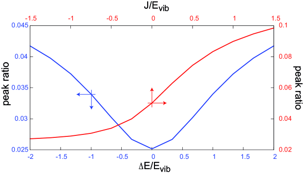
Figure 4: Peak ratios between 0-0 and 0-1 transitions at $T=4$K as a function of $J=J_{\rm DA}$ for $\Delta E/\hbar\omega=1$ and of $\Delta E$ for $J_{\rm DA}/\hbar\omega=-0.5$ (cf. Fig. 3). The arrows mark the uncoupled case (red) and the detuning corresponding to the FMO model (blue). ($E_{\rm vib}=\hbar\omega$)

The ratio between 0-0 and 0-1 emission intensities is investigated in more detail in Fig. 4. For a monomer this ratio would be equal to the Huang-Rhys factor what was used in the calculations, $S=0.05$ in the present case. This value is observed only for $J_{\rm DA}=0$ (marked as a crossing of red arrows in Fig. 4) and for a finite $J_{\rm DA}$ in the limit of large detunings (not shown). At this point we should recall that Huang-Rhys factors and mode frequencies are usually obtained from low-temperature site-selected fluorescence spectra. Clearly, the outcome of such experiment would be influenced by the excitonic coupling. The case of FMO would approximately correspond to the blue curve of the Fig. 4 at the relative detuning -1 marked as a crossing of blue arrows. Our calculations give for that point the ”effective observable” of about S=0.034. We point out that the Huang-Rhys factor obtained from the FMO experiment is smaller than the $S$ reported for BChl in solution. Our calculations give a straightforward explanation of this discrepancy. With the help of our results illustrated in Fig. 4 the Huang-Rhys factors obtained from fluorescence site selection spectroscopy of light-harvesting complexes and other molecular aggregates can be corrected. Obviously the correction can easily be as large as 100%. In case of the FMO in 180 cm^-1 region the observed S should be multiplied by a factor of 1.5. The correction factor becomes smaller for the higher frequency modes. Theoretical studies where the spectral density is extracted from atomic simulations and compared to the fluorescence spectra for benchmarking [25, 55], need to consider these correction factors.

Finally, we note that the measured $S$ values will be reduced in case of negative $J_{\rm DA}$ values (J-aggregate) and increased for the opposite sign (H-aggregate).

4 Summary

We have carried out a thorough comparison of OPA and exact calculations of vibronic excitons in a dimer model. We found that the general behaviour of the calculated absorption spectra are surprisingly similar despite of the radically different energy level structure in the two models. Multi-mode effects have been discussed in dependence on the mode parameters. In the case of negative coupling, which is relevant for the FMO complex, most oscillator strength is concentrated in a transition to a state of essentially electronic character such that no pronounced effect on the spectrum arises. Calculations of the fluorescence spectra show that the Huang Rhys factors obtained from fluorescence spectroscopy of light-harvesting complexes with significant excitonic couplings, need to be corrected. Depending on the excitonic coupling strength and detuning, the correction can be as large as 100%. At the same time, the observed frequencies are not affected if measured at low temperature where the transitions from higher energy levels are not giving any significant contribution.

References

References

- [1] Blankenship R E 2002 Molecular Mechanisms of Photosynthesis (Oxford: Blackwell Science)
- [2] Pullerits T, Sundström V 1996 Acc. Chem. Res. 4842 381
- [3] May V, Kühn O 2011 Charge and Energy Transfer Dynamics in Molecular Systems, Third, Revised and Enlarged Edition (Weinheim: Wiley-VCH)
- [4] Van Amerongen H, Valkunas L, van Grondelle R 2000 Photosynthetic Excitons (Singapore: World Scientific Publishers)
- [5] Renger T, May V, Kühn O 2001 Phys. Rep. 343 137
- [6] Kühn O, Sundström V, Pullerits T 2002 Chem. Phys. 275 15
- [7] Engel G S, Calhoun T, Read E L, Ahn T-K, Mancal T, Cheng Y-C, Blankenship R E, Fleming G R 2007 Nature 446 782
- [8] Collini E, Wong C Y, Wilk K E, Curmi P M G, Brumer P, Scholes G D 2010 Nature 463 644
- [9] Fassioli F, Nazir A, Olaya-Castro A 2010 J. Phys. Chem. Lett. 1 2139
- [10] Ishizaki A, Fleming G R 2009 J. Chem. Phys. 130 234110
- [11] Abramavicius D, Palmieri B, Voronine D V, Sanda F, Mukamel S 2009 Chem. Rev. 109 2350
- [12] Plenio M B, Huelga S F 2008 New J. Phys 10 113019
- [13] Rebentrost P, Mohseni M, Kassal I, Lloyd S, Aspuru-Guzik A 2009 New J. Phys. 11 033003
- [14] Shim S, Rebentrost P, Valleau S, Aspuru-Guzik A 2012 Biophys. J. 102 649
- [15] Huo P, Coker D F 2010 J. Chem. Phys. 133 184108
- [16] Ishizaki A, Fleming G R 2009 Proc. Natl Acad. Sci. USA 106 17255
- [17] Nalbach P, Braun D, Thorwart M 2011 Phys. Rev. E 84 041926
- [18] Brüggemann B, Kjellberg P, Pullerits T 2007 Chem. Phys. Lett. 444 192
- [19] Kjellberg P, Brüggemann B, Pullerits T 2006 Phys. Rev. B 74 024303
- [20] Cheng Y-C, Fleming G R 2008 J. Phys. Chem. A 112 4254
- [21] Chen L, Zheng R, Jing Y, Shi Q 2011 J. Chem. Phys. 134 194508
- [22] Hein B, Kreisbeck C, Kramer T, Rodriguez M 2012 New J. Phys. 14 023018
- [23] Nalbach P, Eckel J, Thorwart M, 2010 New J. Phys. 12 065043
- [24] Abramavicius D, Mukamel S 2011. J. Chem. Phys. 134 174504
- [25] Olbrich C, Strümpfer J, Schulten K, Kleinekathöfer U 2011. J. Phys. Chem. Lett. 2 1771
- [26] Kreisbeck C, Kramer T 2012. J. Phys. Chem. Lett. 3 2828
- [27] Wendling M, Pullerits T, Przyjalgowski M A, Vulto S I E, Aartsma T J, van Grondelle R, van Amerongen H 2000. J. Phys. Chem. B 104 5825
- [28] Rätsep M, Cai Z-L, Reimers J R, Freiberg A 2011. J. Chem. Phys. 134 024506
- [29] Adolphs J, Renger T 2006 Biophys. J. 91 2778
- [30] Polyutov S, Kühn O, Pullerits T 2012 Chem. Phys. 394 21
- [31] Christensson N, Kauffmann H F, Pullerits T, Mančal T 2012 J. Phys. Chem. B 116 7449
- [32] Tiwari V, Peters W K, Jonas D M 2013 Proc. Natl Acad. Sci. USA 110 1203
- [33] Pullerits T, Zigmantas D, Sundström, V 2013 Proc. Natl Acad. Sci. USA 110 1148
- [34] Beenken W, Dahlbom M, Kjellberg P, Pullerits T 2002 J. Chem. Phys. 117 5810
- [35] Dahlbom M, Beenken W, Sundström V, Pullerits T 2002 Chem. Phys. Lett. 364 556
- [36] Schröter M, Kühn O 2013 J. Phys. Chem. A 117 7580
- [37] Brüggemann B, Herek J L, Sundström V, Pullerits T, May V 2001 J. Phys. Chem. B 105 11391
- [38] Brüggemann B, Christensson N, Pullerits T 2009 Chem. Phys. 357 140
- [39] Butkus V, Zigmantas D, Valkunas L, Abramavicius D 2012 Chem. Phys. Lett. 545 40
- [40] Butkus V, Zigmantas D, Abramavicius D, Valkunas L 2013 Chem. Phys. Lett. 587 93
- [41] Chenu A, Christensson N, Kauffmann H, and Mančal T 2013 Scient. Rep. 3 2029
- [42] Seibt J, Hansen T, Pullerits T 2013 J. Phys. Chem. B 117 11124
- [43] Seibt J, Pullerits T 2013 J. Phys. Chem. C 117 18728
- [44] Philpott M R 1971. J. Chem. Phys. 55 2039
- [45] Spano F C 2002 J. Chem. Phys. 116 5877
- [46] Fulton R L, Gouterman M 1961 J. Chem. Phys. 35 1059
- [47] Eisfeld A, Braun L, Strunz W T, Briggs J S, Beck J, Engel V 2005 J. Chem. Phys. 112 134103
- [48] Meyer H-D, Manthe U, Cederbaum L S 1990 Chem. Phys. Lett. 165 73
- [49] Beck M H, Jäckle A, Worth G A, Meyer H-D 2000 Phys. Rep. 324 1
- [50] Seibt J, Winkler T, Renziehausen K, Dehm V, Würthner F, Meyer H-D, Engel V 2009 J. Phys. Chem. A 113 13475
- [51] Ambrosek D, Köhn A, Schulze J, Kühn O 2012 J. Phys. Chem. A 116 11451
- [52] Worth G, Beck M, Meyer H-D The MCTDH Package, Version 8.4, University of Heidelberg: Heidelberg 2007
- [53] Pullerits T, van Mourik F, Monshouwer R, van Grondelle R 1994 J. Luminesc. 58 168
- [54] Milder M T W, Brüggemann B, van Grondelle R, Herek J L 2010 Photosynth. Res. 104 257
- [55] Shim S, Rebentrost P, Valleau S, Aspuru-Guzik A 2012 Biophys. J. 102 649