De Sitter Vacua from Non-perturbative Flux Compactifications

Abstract

We present stable de Sitter solutions of $\mathcal{N}=1$ supergravity in a geometric type IIB duality frame with the addition of non-perturbative contributions. Contrary to the standard approach, we retain the moduli dependence of both the tree level superpotential and its non-perturbative contribution. This provides the possibility for a single-step stabilisation of all moduli simultaneously in a de Sitter vacuum. Using a genetic algorithm we find explicit solutions with different features.

Introduction. The importance of accelerating space-times in cosmology, both for inflation and dark energy, makes it critical to understand the role of de Sitter (dS) vacua in string theory. Many such constructions have been criticised as being rather ad-hoc. In the KKLT set-up Kachru et al. (2003), one adds a non-perturbative contribution as well as explicit, supersymmetry-breaking uplift terms to achieve a dS vacuum. These are necessary additions to $\mathcal{N}=1$ compactifications with only IIB gauge fluxes, which only lead to Minkowski vacua with flat directions Giddings et al. (2002). On the IIA side, the situation regarding moduli stabilisation is better, as the inclusion of gauge fluxes alone leads to AdS vacua DeWolfe et al. (2005). However, it is not possible to obtain dS solutions in this vein Hertzberg et al. (2007). Adding metric-fluxes does lead to dS solutions Caviezel et al. (2009); Flauger et al. (2009), but all known examples are unstable. In this Letter, we show that geometric and isotropic fluxes with non-perturbative contributions are enough to stabilise simultaneously all moduli in a dS vacuum, in the simplest scenario possible, widening the dS landscape.

We focus on a $T^{6}/(\mathbb{Z}_{2}\times\mathbb{Z}_{2})$ compactification with fluxes in type IIB supergravity in ten dimensions. The number of untwisted moduli is $(h^{(1,1)},h^{(2,1)})=(3,3)$ plus the dilaton. We concentrate on the isotropic case with a single Kähler and complex structure moduli, that is, an $STU$-type of model. The Kähler potential takes the form:

$$K=-\log[-i(S-\bar{S})]-3\log[-i(T-\bar{T})]-3\log[-i(U-\bar{U})].$$ (1)

The scalar potential takes the usual form (we are setting $M_{P}^{-2}=8\pi G=1$):

$$V=e^{K}\left(K^{I\bar{J}}D_{I}WD_{\bar{J}}\overline{W}-3|W|^{2}\right),$$ (2)

$D_{I}W=\partial_{I}W+\partial_{I}KW$ with $I,J$ labelling all moduli.

The tree-level superpotential depends on the dilaton $S$ and complex structure $U$ (jointly referred to as complex structure moduli). These are generated by the presence of RR-flux $F_{3}$ and NSNS-flux $H_{3}$ (with coefficients $a_{i}$, $b_{i}$, respectively):

$$W_{tree}=P(a_{i},U)-SP(b_{i},U)\,,$$ (3)

where $P(f_{i},U)$ are polynomials in $U$ of the form

$$P(f_{i},U)=f_{0}-3f_{1}U+3f_{2}U^{2}-f_{3}U^{3}\,.$$ (4)

Thus, these fluxes generate a potential for the complex structure moduli stabilising them Giddings et al. (2002). However, the Kähler modulus remains as a flat direction.

To stabilise the $T$-modulus, the standard approach has been to first use the tree-level flux contributions to fix $S$ and $U$ in a SUSY vacuum. Second, introduce a non-perturbative term $W_{\textrm{NP}}(T)$ for the Kähler modulus, allowing its stabilisation. It is assumed that the first step results in a constant contribution to the superpotential, $W_{0}=$const. and a constant coefficient for the non-perturbative term, $A_{0}=$const.:

$$W=W_{0}+A_{0}\,e^{ixT}\,,$$ (5)

where $x=2\pi/K$ for gaugino condensation with gauge group rank $K$. Using this superpotential, only AdS minima can be obtained. Therefore, a final third step has been taken by adding a suitable uplifting term Kachru et al. (2003), lifting the AdS minimum to a dS.

This three-step process has been criticised in the literature since in general, not only $W_{0}$ but also the coefficient $A_{0}$ depend on the complex structure moduli Witten (1996). Therefore the second step can lead to complications since heavy modes could mix with light modes de Alwis (2005a, b) and create instabilities Choi et al. (2004) (see however Gallego and Serone (2009) for a discussion on the consistency conditions for this step). Moreover, adding an uplifting term by hand is under limited theoretical control (e.g. adding an anti-brane is an explicit heavy breaking of supersymmetry and it is not clear that one can still use a supergravity description). An alternative was proposed to uplift using D-terms in Burgess et al. (2003); Achucarro et al. (2006). Finally, the third step has been relaxed in Covi et al. (2009), where it was shown how to obtain dS minima without the need of an artificial uplifting term. However the second step has been so far assumed in order to obtain stabilisation of all moduli. This Letter addresses the natural question whether a single-step process can give rise to (meta-)stable dS vacua, stabilising all moduli simultaneously, even in simple models.

A novel mechanism of moduli stabilisation. To study this possibility, we consider the usual tree-level superpotential augmented with a non-perturbative term. The coefficient of the latter will generically depend on the complex structure moduli $S$ and $U$ in a non-trivial but unknown way. Following the reasoning for non-geometric fluxes of Shelton et al. (2005), it seems natural to model this dependence in a way that respects the $S$ and $U$ duality covariance. This leads to the following Ansatz:

$$W=W_{tree}+\left[P(\tilde{a}_{i},U)-P(\tilde{b}_{i},U)S\right]e^{ixT},$$ (6)

where all four polynomials have the structure (4). Although we do not provide a rigorous derivation of this moduli dependence in the non-perturbative term, it is constrained to be such a polynomial in $S,U$ by duality arguments; indeed a similar form has been studied in an explicit string theory setting Uranga (2009). An alternative interpretation of this Ansatz is that the polynomials represent a Taylor expansion in terms of small $S,U$, as we will justify below.

The coefficients of the non-perturbative term appear in complete analogy with the gauge fluxes in the superpotential. Thus we refer to $\tilde{a}_{i}$ and $\tilde{b}_{i}$ as non-perturbative fluxes. This leads to a total set of 16 fluxes. However, as we explain later, it will be sufficient to have 12 fluxes. We therefore set the fourth polynomial equal to zero.

To find solutions, we use the property that any solution to the equations of motion can be represented by a solution in the origin of moduli space (in our conventions located at $S=T=U=i$ with $x=1$). This technique was first proposed in the context of half-maximal supergravity Dibitetto et al. (2011) and subsequently used to explore the vacuum structure of maximal supergravity Dall’Agata and Inverso (2012); Borghese et al. (2012), but can be applied to any theory with a homogeneous scalar manifold. This avoids an over-counting of solutions and reduces dramatically the complexity of the equations of motion. While these in general can be high-degree polynomials for the fields, in the origin these reduce to quadratic equations in terms of fluxes. Solutions correspond to flux configurations for which these quadratic combinations vanish. The origin is however not a configuration that should be considered a valid supergravity limit, since the volume of the internal space and the string coupling are both equal to one. Below we explain how to deal with this issue.

To solve the resulting quadratic equations in the fluxes $\{a_{i},b_{i},\tilde{a}_{i}\}$, we use the fact that when supersymmetry is preserved, the equations of motion are implied Danielsson and Dibitetto (2013b):

$$D_{I}W\equiv A_{I}+iB_{I}=0\quad\Rightarrow\quad\partial_{I}V=0,$$ (7)

where the six supersymmetry breaking (SUSY) parameters $A_{I}$ and $B_{I}$ are linear combinations of the superpotential couplings $\{a_{i},b_{i},\tilde{a}_{i}\}$. It will be advantageous to split up the latter in (linear combinations of) two sets: there are six SUSY parameters while the orthogonal combinations preserve SUSY. Via this approach, in general all moduli take part in SUSY and contribute to the uplifting of the potential. This is to be contrasted to for example Kachru et al. (2003), where uplifting is only considered in the direction of Im($T$) while $S$ and $U$ are in SUSY minima.

Next, one exploits the fact that the equations of motion are implied by SUSY. Therefore, the equations of motion become quadratic in the SUSY parameters or bilinear in the SUSY and SUSY parameters. For this to work, the total set of parameters must be at least equal to twice the number of (real) fields, in our case $6+6=12$. Type IIB tree-level flux contributions to the superpotential consists of $8$ parameters $a_{i},b_{i}$ (3, 4). In Danielsson and Dibitetto (2013b) the extra couplings were taken to be so called non-geometric fluxes. Here, we add the non-perturbative fluxes $\tilde{a}_{i}$ (6).

Given these sets of solutions parameterised by the six SUSY parameters, we follow Blåbäck et al. (2013a) in using a genetic algorithm to scan this parameter space to look for stable dS solutions (for similar applications of genetic algorithms see Damian et al. (2013); Damian and Loaiza-Brito (2013); Blåbäck et al. (2013b)). We thus require both the cosmological constant as well as all the scalar masses, obtained by diagonalising the mass matrix

$$(m^{2})^{I}_{J}=\frac{K^{IK}\partial_{K}\partial_{J}V}{V}\,,$$ (8)

to be positive.

Perturbative reliability. In order to get to a regime for the values of the moduli that is a reliable supergravity approximation of string theory, we need to ensure that we work at large volume and small string coupling, such that higher string mode contributions and loop corrections are suppressed: a) Large volume: ${\cal V}\sim r^{6}\gg 1$ . b) Small string coupling: $g_{s}^{-1}\gg 1$, where ${\cal V}=\textrm{Vol.}/\ell_{s}$ with $\ell_{s}$ the string scale, and we have introduced a characteristic (dimensionless) radius of the internal space, $r$. The volume is further given in terms of the overall Kähler modulus as ${\rm Im}\,T={\cal V}^{2/3}$ and the string coupling in terms of the dilation as $g_{s}=({\rm Im}\,S)^{-1}$.

Consider the following rescaling of the volume and the string coupling $r\to N^{\alpha}r,\quad g_{s}\to N^{-\beta}g_{s},$ for $\alpha$ and $\beta$ some positive numbers with $N\gg 1$. From the expression for the scalar potential, the fluxes and $x$ have to be rescaled as:

$$a_{i},\tilde{a}_{i} \to N^{6\alpha+\beta/2+\gamma}\,a_{i},\tilde{a}_{i}\,,\qquad x\to N^{-4\alpha}\,x\,,$$

$$b_{i} \to N^{6\alpha-\beta/2+\gamma}\,b_{i}\,,$$ (9)

for the solution to be preserved. We have also introduced a parameter $\gamma$ that represents an overall scaling of the fluxes that is always possible to perform. The potential scales as $V\to N^{2\gamma}\,V\,,$ and the normalised masses remain invariant. For the special case of gaugino condensation, where $x=\frac{2\pi}{K}$, the scaling (9) implies that we need to scale $K$ as: $K\to N^{4\alpha}\,K\,.$

Given a solution, we can achieve a large volume and small string coupling regime, via a suitable rescaling of the parameters. A drawback may be that this rescaling requires a small value of the parameter $x$, which in the case of gaugino condensation, translates into a large rank of the gauge group $K$. In the context of non-compact Calabi-Yaus, it has been discussed that arbitrarily high gauge group ranks are possible Gukov et al. (2000). In the compact case the situation turns out to be more restrictive, but relatively large values are possible Louis et al. (2012).

Finally, we should also consider the tadpole cancellation condition, which is a quadratic combination of flux parameters, $H_{3}\wedge F_{3}$:

$$N_{\textrm{D}3}=a_{3}b_{0}-3a_{2}b_{1}+3a_{1}b_{2}-a_{0}b_{3},$$ (10)

scaling according to $N_{\textrm{D}3}\to N^{12\alpha+2\gamma}\,N_{\textrm{D}3}.$ As the tadpole is bounded from below by the orientifold contribution, one should worry about this rescaling in the case of negative $N_{\textrm{D}3}$. Indeed, in all our examples below, the tadpole will be negative. In order to avoid that the large volume limit pushes the tadpole below its lower limit, one can choose the $\gamma$ parameter suitably.

Notice that there is no particular requirement of the value for the complex structure modulus $U$ at the minimum. Therefore, we keep this field to the origin. However, we could rescale it as well to small values in such a way that the power expansion in the non-perturbative function $P_{3}$ can be truncated at the third power consistently.

We next consider the relevance of possible perturbative corrections to the Kähler potential since these could dominate over the non-perturbative contributions to the superpotential, rendering the present set-up inconsistent. Perturbative contributions scale with $K_{\rm P}\sim 1/({\cal V}g_{s}^{3/2})$. Since our method to find solutions starts with all fields at the origin and fluxes of the same order, all contributions in the superpotential are of the same order. After making the above described rescalings, all terms in the potential scale in the same way and once perturbative Kähler contributions are added, we can write

$$V_{\textrm{full}}\to N^{2\gamma}\left(V+K_{\textrm{P}}V\right)\sim N^{2\gamma}\left(V+N^{-6\alpha+\frac{3\beta}{2}}V\right),$$ (11)

hence $K_{\textrm{P}}$ contributions will be suppressed with a factor $N^{-6\alpha+\frac{3\beta}{2}}$ compared to the potential calculated here. We can therefore safely neglect these by a suitable choice of $\alpha,\beta$.

Explicit de Sitter solutions. We performed five individual searches where additional criteria were required. These additional criteria were chosen to be:

$1,2:$ maximize and minimize $\tilde{\gamma}=|DW|^{2}/(3|W|^{2})$ (while keeping $\tilde{\gamma}>1$),

$3,4:$ maximize and minimize the scale between the fluxes $|b_{i}|/|a_{i}|$,

$5:$ minimize the scale between the fluxes $|\tilde{a}_{i}|/|a_{i}|$.

	Sol. 1	Sol. 2	Sol. 3	Sol. 4	Sol. 5
$V_{0}$	$0.00113$	$2.23\times 10^{-12}$	$0.0000251$	$0.0000234$	$8.61\times 10^{-12}$
$\tilde{\gamma}-1$	$0.0256$	$5.11\times 10^{-11}$	$0.00248$	$0.0160$	$6.05\times 10^{-10}$
$\frac{|b_{i}|}{|a_{i}|}$	$0.298$	$0.599$	$1.32$	$0.208$	$0.997$
$\frac{|\tilde{a}_{i}|}{|a_{i}|}$	$0.611$	$0.274$	$0.528$	$0.621$	$0.000227$
Masses	$\begin{array}[]{c}39.0\\ 19.7\\ 12.4\\ 9.74\\ 0.00236\\ 0.0000747\\ \end{array}$	$\begin{array}[]{c}2.11\times 10^{10}\\ 8.71\times 10^{9}\\ 7.00\times 10^{9}\\ 3.41\times 10^{9}\\ 1.26\times 10^{9}\\ 6.01\times 10^{8}\\ \end{array}$	$\begin{array}[]{c}1140.\\ 387.\\ 106.\\ 18.4\\ 6.16\\ 0.0000612\\ \end{array}$	$\begin{array}[]{c}76.2\\ 36.0\\ 19.6\\ 11.4\\ 0.774\\ 0.000252\\ \end{array}$	$\begin{array}[]{c}2.20\times 10^{9}\\ 9.80\times 10^{8}\\ 2.45\times 10^{8}\\ 490000.\\ 101000.\\ 100000.\\ \end{array}$

Table 1: Properties of the solutions. The masses are normalised with the potential and all scales are given in Planck units.

The main properties of our solutions are presented in Table 1, while the SUSY parameters for these solutions can be found in Table 2. A number of general features can be extracted from these examples. Firstly, it follows that the SUSY and AdS scales are always of the same order and cannot be separated. The maximum ratio between the scales is $\approx 1.0256$, as follows from solution 1. Similarly, one can approach a ratio equal to one with very good accuracy, as illustrated by solution 2. Another observation from this solution is that the lowest mass can be made very large compared to the potential energy $V_{0}$. Finally, as the flux parameters are of decreasing order,

$$\{\tilde{a}_{0},\tilde{a}_{1},\tilde{a}_{2},\tilde{a}_{3}\}\approx\{0.0835,0.0702,0.0372,0.00921\}$$ (12)

the small-$U$ expansion of (6) is justified in this case.

A second point is that we tried to achieve a hierarchy between the RR- and NSNS-fluxes. The reason for doing so is the small coupling limit; as the rescaling (9) acts different on these two set of fluxes, we would like to start off with a hierarchy of values for these. After the rescaling we end up at small coupling with fluxes of the same order. As can be seen from solutions 3 and 4, it is possible to achieve a small degree of separation between the two sets of fluxes. However this separation is only due to large contributions from the non-perturbative fluxes.

Finally, in solution 5 we were able to create a hierarchy between the perturbative and non-perturbative fluxes. This hierarchy is only possible to achieve with the loss of a hierarchy of the NSNS and RR sector. The reason for this lies in the structure of the equation of motion for $S$. On the level of the perturbative superpotential this equation forces the so-called imaginary self-dual (ISD) condition for the flux $G_{3}=F_{3}+SH_{3}$ Giddings et al. (2002). Via the addition of small non-perturbative contributions it is only possible to perturb this condition. This is why we see in solutions 3 and 4 that the non-perturbative terms contribute much more than in solution 5. For the same reason, i.e. small non-perturbative contributions cannot significantly change the ISD condition, we are not able to find solutions without net O-planes, as is argued to be possible in type IIA Danielsson and Dibitetto (2013a).

For the most interesting solution 5, we observe also that because the non-perturbative contributions are suppressed, one may expect a separation of masses among $S,U$ and $T$. Indeed the last two smallest masses in Table 1 correspond to the eigenvectors which are dominated by the real and imaginary parts of $T$. The other small mass corresponds mostly to a combination of the $S,U$ axions. Moreover, the lowest mass is still significantly larger than the potential.

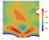
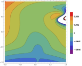
Figure 1: The stability (non-normalised mass) (left) and dS (right) landscape of Sol.$~{}2$. The solution is located at the origin. The pictures are a 2D slice of the parameters $x=-e(9B_{1}-2B_{2}-B_{2})/2$ and $y=-e(7A_{1}-2A_{2}-A_{3})/6$ that are part of a linear combination of $A_{I},B_{I}$ in eq. (7).

Finally, it is interesting to consider the interplay between stability and dS solutions. For non-geometric stable dS solutions, the intersection of stability and dS overlap is thin sheets because of small differences in the shape of these landscapes Danielsson and Dibitetto (2013b), thus requiring fine-tuning. This is not the case for the present non-perturbative solutions. The stability and potential landscapes, plotted in Figure 1, have noticeably different shapes. This implies that there are sizeable intersection regions.

This non-trivial overlap will be important when taking flux quantisation into account. By scaling $N$ large, the parameters $A_{I}$ and $B_{I}$ become approximately integers. One can then make $a_{i},b_{i}$ integers by an appropriate truncation. This will slightly modify the solution, (inversely) related to order to which we rescale $N$. However, because of the large intersection areas of stability and dS, only a very coarse truncation would significantly modify the solution and possibly spoil stability and/or dS. In our case, where the orientifold tadpole gives a bound on how much rescaling can take place, the truncation would have to be indeed quite coarse. On account of the large stable dS regions, one can achieve quantisation without losing stability nor positive potential energy. We have explicitly checked this for solution 5, which can be rescaled and truncated to the flux parameters

$$\{a_{0},a_{1},a_{2},a_{3},b_{0},b_{1},b_{2},b_{3}\}=\{-1,4,1,-12,4,0,-1,0\}\,,$$ (13)

which gives a tadpole $N_{O3}=60$ and rank $K=67$. This has a stable dS solution at

$$\!\!\{S,T,U\} \!\approx\! \{\!.00616\!+\!ie^{1.32},-.000456\!+\!ie^{2.63},-.117\!+\!ie^{.0728}\}$$

which is a perturbation of our solution 5.

Discussion. In summary, we considered a novel one-step mechanism to stabilise all geometric moduli of type IIB toroidal compactifications in a dS vacuum, using the non-trivial moduli dependence of the tree-level superpotential and the non-perturbative contributions. The latter is motivated by duality invariance of string theory, and can also be seen as a small-field expansion. Our approach improves the three-step KKLT mechanism by including the complex structure in the non-perturbative piece allowing us to stabilise all moduli at once in a dS vacua, avoiding also the introduction of explicitly SUSY terms, such as anti-D-branes. We have presented a number of explicit stable dS solutions, amongst one with quantised fluxes.

We view our results as very compelling arguments to extend the dS landscape in type IIB flux compactifications. They represent a first step towards a new direction allowing for a more complete landscape of stable dS vacua.

Acknowledgements. The authors would like to thank Ulf Danielsson, Giuseppe Dibitetto, Marc Andre Heller, Thomas Van Riet and Bert Vercnocke for useful discussions. JB acknowledges support by the Swedish Research Council (VR) and the Göran Gustafsson Foundation.

	Sol. 1	Sol. 2	Sol. 3	Sol. 4	Sol. 5
$A_{1}$	$-0.147286$	$-0.0859982$	$0.0590861$	$-0.0115235$	$0.000516097$
$A_{2}$	$0.449418$	$-1.58993$	$-0.483429$	$0.165447$	$1.15243$
$A_{3}$	$-0.907814$	$0.4631$	$-0.131249$	$-0.144582$	$-0.000587804$
$B_{1}$	$0.377918$	$-0.236806$	$0.0870739$	$0.0793589$	$0.00319387$
$B_{2}$	$1.6678$	$-1.12127$	$0.826607$	$0.259372$	$-0.196848$
$B_{3}$	$0.173821$	$-0.047207$	$-0.0614712$	$0.0902761$	$-0.00969035$

Table 2: These are the values of the SUSY parameters defined by (7) that gives the solutions displayed in Table 1 (rounded to six digits).

References

- Kachru et al. (2003) S. Kachru, R. Kallosh, A. D. Linde, and S. P. Trivedi, Phys.Rev. D68, 046005 (2003), arXiv:hep-th/0301240 [hep-th] .
- Giddings et al. (2002) S. B. Giddings, S. Kachru, and J. Polchinski, Phys.Rev. D66, 106006 (2002), arXiv:hep-th/0105097 [hep-th] .
- DeWolfe et al. (2005) O. DeWolfe, A. Giryavets, S. Kachru, and W. Taylor, JHEP 0507, 066 (2005), arXiv:hep-th/0505160 [hep-th] .
- Hertzberg et al. (2007) M. P. Hertzberg, S. Kachru, W. Taylor, and M. Tegmark, JHEP 0712, 095 (2007), arXiv:0711.2512 [hep-th] .
- Caviezel et al. (2009) C. Caviezel, P. Koerber, S. Kors, D. Lust, T. Wrase, et al., JHEP 0904, 010 (2009), arXiv:0812.3551 [hep-th] .
- Flauger et al. (2009) R. Flauger, S. Paban, D. Robbins, and T. Wrase, Phys.Rev. D79, 086011 (2009), arXiv:0812.3886 [hep-th] .
- Witten (1996) E. Witten, Nucl.Phys. B474, 343 (1996), arXiv:hep-th/9604030 [hep-th] .
- de Alwis (2005a) S. de Alwis, Phys.Lett. B626, 223 (2005a), arXiv:hep-th/0506266 [hep-th] .
- de Alwis (2005b) S. de Alwis, Phys.Lett. B628, 183 (2005b), arXiv:hep-th/0506267 [hep-th] .
- Choi et al. (2004) K. Choi, A. Falkowski, H. P. Nilles, M. Olechowski, and S. Pokorski, JHEP 0411, 076 (2004), arXiv:hep-th/0411066 [hep-th] .
- Gallego and Serone (2009) D. Gallego and M. Serone, JHEP 0901, 056 (2009), arXiv:0812.0369 [hep-th] .
- Burgess et al. (2003) C. Burgess, R. Kallosh, and F. Quevedo, JHEP 0310, 056 (2003), arXiv:hep-th/0309187 [hep-th] .
- Achucarro et al. (2006) A. Achucarro, B. de Carlos, J. Casas, and L. Doplicher, JHEP 0606, 014 (2006), arXiv:hep-th/0601190 [hep-th] .
- Covi et al. (2009) L. Covi, M. Gomez-Reino, C. Gross, G. A. Palma, and C. A. Scrucca, JHEP 0903, 146 (2009), arXiv:0812.3864 [hep-th] .
- Cicoli et al. (2012a) M. Cicoli, A. Maharana, F. Quevedo, and C. Burgess, JHEP 1206, 011 (2012a), arXiv:1203.1750 [hep-th] .
- Louis et al. (2012) J. Louis, M. Rummel, R. Valandro, and A. Westphal, JHEP 1210, 163 (2012), arXiv:1208.3208 [hep-th] .
- Parameswaran et al. (2011) S. L. Parameswaran, S. Ramos-Sanchez, and I. Zavala, JHEP 1101, 071 (2011), arXiv:1009.3931 [hep-th] .
- Balasubramanian et al. (2005) V. Balasubramanian, P. Berglund, J. P. Conlon, and F. Quevedo, JHEP 0503, 007 (2005), arXiv:hep-th/0502058 [hep-th] .
- Cicoli et al. (2012b) M. Cicoli, S. Krippendorf, C. Mayrhofer, F. Quevedo, and R. Valandro, JHEP 1209, 019 (2012b), arXiv:1206.5237 [hep-th] .
- Cicoli et al. (2013a) M. Cicoli, S. Krippendorf, C. Mayrhofer, F. Quevedo, and R. Valandro, JHEP 1307, 150 (2013a), arXiv:1304.0022 [hep-th] .
- Cicoli et al. (2013b) M. Cicoli, D. Klevers, S. Krippendorf, C. Mayrhofer, F. Quevedo, et al., (2013b), arXiv:1312.0014 [hep-th] .
- Danielsson and Dibitetto (2013a) U. Danielsson and G. Dibitetto, (2013a), arXiv:1312.5331 [hep-th] .
- Shelton et al. (2005) J. Shelton, W. Taylor, and B. Wecht, JHEP 0510, 085 (2005), arXiv:hep-th/0508133 [hep-th] .
- de Carlos et al. (2010) B. de Carlos, A. Guarino, and J. M. Moreno, JHEP 1002, 076 (2010), arXiv:0911.2876 [hep-th] .
- Uranga (2009) A. M. Uranga, JHEP 0901, 048 (2009), arXiv:0808.2918 [hep-th] .
- Dibitetto et al. (2011) G. Dibitetto, A. Guarino, and D. Roest, JHEP 1103, 137 (2011), arXiv:1102.0239 [hep-th] .
- Dall’Agata and Inverso (2012) G. Dall’Agata and G. Inverso, Nucl.Phys. B859, 70 (2012), arXiv:1112.3345 [hep-th] .
- Borghese et al. (2012) A. Borghese, A. Guarino, and D. Roest, JHEP 1212, 108 (2012), arXiv:1209.3003 [hep-th] .
- Danielsson and Dibitetto (2013b) U. Danielsson and G. Dibitetto, JHEP 1303, 018 (2013b), arXiv:1212.4984 [hep-th] .
- Blåbäck et al. (2013a) J. Blåbäck, U. Danielsson, and G. Dibitetto, JHEP 1308, 054 (2013a), arXiv:1301.7073 [hep-th] .
- Damian et al. (2013) C. Damian, L. R. Diaz-Barron, O. Loaiza-Brito, and M. Sabido, JHEP 1306, 109 (2013), arXiv:1302.0529 [hep-th] .
- Damian and Loaiza-Brito (2013) C. Damian and O. Loaiza-Brito, Phys.Rev. D88, 046008 (2013), arXiv:1304.0792 [hep-th] .
- Blåbäck et al. (2013b) J. Blåbäck, U. Danielsson, and G. Dibitetto, (2013b), arXiv:1310.8300 [hep-th] .
- Gukov et al. (2000) S. Gukov, C. Vafa, and E. Witten, Nucl.Phys. B584, 69 (2000), arXiv:hep-th/9906070 [hep-th] .