Constraining the Variation in Fine-Structure Constant Using SDSS DR8 QSO Spectra

Abstract

We report a robust constrain on the possible variation of fine-structure constant, $\alpha\equiv e^{2}/\hbar c$, obtained using O iii $\lambda\lambda$ 4959,5007 nebular emission lines from QSOs.We find a $\Delta\alpha/\alpha=-(2.1\pm 1.6)\times 10^{-5}$ based on a well selected sample of 2347 QSOs from Sloan Digital Sky Survey Data Release 8 with 0.02 $<z<$ 0.74. Our result is consistent with a non-varying $\alpha$ at a level of $2\times 10^{-5}$ over approximately 7 Gyr. This is the largest sample of extragalactic objects yet used to constrain the variation of $\alpha$. While this constraint is not as stringent as those determined using many-multiplet method it is free from various systematic effects. A factor of $\sim$ 4 improvement in $\Delta\alpha/\alpha$ achieved here compared to the previous study (Bahcall et al., 2004) is just consistent with what is expected based on a factor of 14 times bigger sample used here. This suggests that errors are mainly dominated by the statistical uncertainty. We also find the ratio of transition probabilities corresponding to the O iii $\lambda$5007 and $\lambda$4959 lines to be 2.933$\pm$0.002, in good agreement with the National Institute of Standards and Technology measurements.

1 Introduction

Most of the physical theories rely on a set of fundamental constants (e.g. fine-structure constant, $\alpha$ = $e^{2}/\hbar c$, proton-to-electron mass ratio, $\mu$, etc.) that can not be calculated theoretically and have to be measured experimentally. However, unified theories of particle interaction like string theory suggest the spatial and temporal variation of these fundamental constants (see Uzan, 2003; Uzan et al., 2011). Most of the laboratory measurements are consistent with the no variation of physical constants over time-scales of $\lesssim 100$ yr (e.g. Rosenband et al., 2008; Guéna et al., 2012). For example, the constancy of $\alpha$ has been established via extremely accurate laboratory measurements extending over 16 years resulting in $\dot{\alpha}/\alpha<$ 10^-16 yr^-1 (Guéna et al., 2012). The study of geological samples have also shown a non-varying physical constants over time-scales of two billion years (e.g. Petrov et al., 2006). Spectra of high-$z$ QSOs, in principle allow one to probe possible variations of dimensionless fundamental constants over cosmological scales.

Initial attempts to measure $\alpha$ at high redshifts were based on the relative separation of Alkali-Doublet (AD) lines (Savedoff, 1956; Bahcall & Schmidt, 1967; Wolfe et al., 1976; Levshakov, 1994; Varshalovich et al., 1996; Cowie & Songaila, 1995; Varshalovich et al., 2000; Murphy et al., 2001; Chand et al., 2005). Chand et al. (2005) used a sample of 23 Si iv absorbers, observed with Very Large Telescope Ultraviolet and Visual Echelle Spectrograph (VLT/UVES), to find $\Delta\alpha/\alpha$ = $-(0.02\pm 0.55)\times 10^{-5}$ which is the best constraint on $\Delta\alpha/\alpha$ based on AD method. Higher sensitivities in $\Delta\alpha/\alpha$ ($\lesssim 10^{-5}$) can be achieved using Many-Multiplet (MM) method in which one simultaneously correlates different multiplets from several ions (Dzuba et al., 1999a, b; Webb et al., 1999). Murphy et al. (2003) applied the MM technique on a sample of 128 QSO absorbers observed with High Resolution Echelle Spectrometer (HIRES) on Keck to find a $\Delta\alpha/\alpha$ = $-5.7\pm 1.0$ ppm which shows $\alpha$ is smaller at higher redshifts. On the contrary, the analysis of a VLT/UVES sample of 21 Mg ii systems by Srianand et al. (2007) resulted in a $\Delta\alpha/\alpha$ = $+0.1\pm 1.5$ ppm, consistent with a no variation in $\alpha$ at high redshifts. Null results are also obtained using only Fe ii multiplets of few individual systems (Quast et al., 2004; Chand et al., 2006; Levshakov et al., 2007). Webb et al. (2011) compiled a large sample of QSOs from both Keck/HIRES and VLT/UVES to claim a spatially varying $\alpha$ with a dipole pattern. This claim is not yet verified independently (see for example, Molaro et al., 2013). Although using MM method one reaches high sensitivities in $\Delta\alpha/\alpha$  it is possible that this method may suffer from systematics related to ionization and chemical homogeneities. In addition it has also been found that different high resolution spectroscopic data used presently suffer from large and small scale wavelength calibration errors (Griest et al., 2010; Whitmore et al., 2010; Rahmani et al., 2013). Therefore, it is important to have independent measurements using different instruments and measurement techniques. Stringent constraint on fundamental constants can be obtained by comparing the 21-cm redshift with that of UV lines. Applying such a techniques on a sample of four Mg ii absorbers Rahmani et al. (2012) found a $\Delta\alpha/\alpha$ = $0.0\pm 1.5$ ppm, consistent with no variation in $\alpha$. The major uncertainty in this technique comes from the difficulties in associating the 21-cm component with the corresponding UV absorption line component.

O iii  $\lambda\lambda 4959,5007$ are two strong nebular emissions, with a doublet separation of $\Delta\lambda_{\rm OIII}=47.9320$ Å, seen in the spectrum of most of the QSOs and star-forming galaxies. A comparison between the laboratory value of $\Delta\lambda_{\rm OIII}$ and its value measured from a QSO leads to a constraint on $\Delta\alpha/\alpha$  in the range of $10^{-4}$–$10^{-3}$. Bahcall et al. (2004) applied such a technique on 165 well selected QSO spectra published by Sloan Digital Sky Survey (SDSS) Data Release one (DR1) to find $\Delta\alpha/\alpha$ = $+(1.2\pm 0.7)\times 10^{-4}$. In this work, we apply the same technique to a much larger sample of QSOs available in SDSS DR8 (Aihara et al., 2011) to obtain a stringent constrain on the value of $\alpha$. In contrary to absorption line techniques, the effect of systematic errors will be minimized due to the large sample of available QSOs. Star-forming galaxies are also suitable for such studies as they have narrow O iii emission lines that are hardly contaminated by broad H$\beta$ emission as frequently seen in QSOs. However, we have chosen QSOs as they spread over much larger redshifts than galaxies and also have a well defined power-law continuum that makes the analysis using automated procedures more straightforward. Furthermore, intrinsic emission line profiles of galaxies are not usually resolved in the SDSS spectra. This makes the estimate of the line centroids to be dominated by the systematic errors. This paper is organized as follows. In section 2 we explain our sample of QSO. We present our algorithm for measuring $\Delta\alpha/\alpha$ from each QSO in section 3. Results and conclusions are presented in section 4 and 5, respectively.

2 QSO Sample

The QSO sample used in this study comes from the spectroscopic sample of QSOs published by SDSS DR8 (Aihara et al., 2011). We begin with a sub-sample of SDSS DR8 QSOs with $z\leq$ 0.74. At $z\gtrsim 0.74$, the O iii doublet falls at the observed wavelength of $\gtrsim$ 8712 Å where the SDSS spectrum is usually filled with lots of spikes most likely due to residuals from subtraction of strong sky emission lines. As our exercise requires very high quality data we have excluded QSOs with their O iii emission in these regions. There are 26368 QSOs within the redshift range considered above. We further notice that a significant fraction of QSOs have poor spectral quality close to O iii emission lines that can lead to highly unreliable $\Delta\alpha/\alpha$ measurements. It is important to exclude such systems from our analysis. By trying different filters we found that the following set of conditions can confidently reject the majority of such QSOs: (i) The amplitude of O iii $\lambda 4959$ emission, $A_{1}$, must be larger than five times of the average error; (ii) The amplitude-ratio of O iii $\lambda 5007$ to O iii $\lambda 4959$ emission, $A_{2}/A_{1}$, must be greater than 1. Ideally, $A_{2}/A_{1}\sim 3$; (iii) There should not be any pixel with bad flag in wavelength range of O iii lines; (iv) The O iii doublets should not be so broad that their profiles overlap. We implement this by considering those doublet where $5\sigma<(\lambda_{2}-\lambda_{1})/2$ where $\sigma$ is the width of the best fitted Gaussian to O iii emissions. The preliminary cuts are very modest to remove only the worst spectra. The remaining 12016 QSO spectra can still have various problems which makes them not ideally suited for $\Delta\alpha/\alpha$ measurements. We now apply additional selection filters suggested by Bahcall et al. (2004) to further prune our sample.

2.1 Signal-to-noise ratio of O iii emission

To have precise measurements we need a very clean detection of O iii emission lines. O iii doublets with poor SNR can lead to $\Delta\alpha/\alpha$ measurements with large systematic errors. To choose QSO spectra with clean O iii emission lines we accept only those QSOs having O iii fluxes detected with a SNR of at least 15. Here we calculate the noise from the scatter of the flux in the line free region used to fit the continuum in the vicinity of the O iii emission lines. This cut leaves us with 8721 QSOs.

2.2 Broad H$\beta$ emission

H$\beta$ $\lambda$4861 line is the closest emission line to the O iii $\lambda$4959 line. It is very well known that H$\beta$ emission is usually broad. A very broad H$\beta$ line, which is frequently seen in QSOs spectra, can distort the emission profile of O iii $\lambda$4959 and can lead to wrong $\alpha$ measurements. We require to find a condition based on which we can check if the emission profile of H$\beta$ has significant overlap with the O iii $\lambda$4959 profile. To do so we only accept QSOs that pass the following two conditions: (i) equivalent width (EW) of H$\beta$ is two time smaller than the EW of O iii $\lambda$5007; (ii) fraction of H$\beta$ flux that overlaps with O iii $\lambda$4959 to be less than 2%. Only 4707 out of 8721 QSOs pass through such a filter.

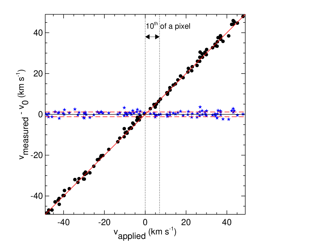
Figure 1: Result of simulations to check the accuracy of our cross-correlation analysis. The abscissa is the applied shift and the ordinate is the mean of the measured shifts for 100 realizations. On the solid line the measured and applied shifts are equal. The asterisks are the residuals (measured - applied) and the long dashed lines are the mean and 1$\sigma$ scatter of the residuals. The two vertical dashed lines indicate 1/10^th of a pixel size ($\Delta$v $\sim$ 7 km s^-1).

2.3 Kolmogorov-Smirnov Test

The estimated value of $\Delta\alpha/\alpha$ is very sensitive to the shape of the O iii doublet emission profiles. Therefore, any mismatch between the shapes of the doublet emissions (due to unknown contamination) can lead to a wrong $\Delta\alpha/\alpha$ measurement. Here we make use of a seven point Kolmogorov-Smirov (KS) test to quantify the similarity between the shapes of the two O iii emission lines. To do so we determine whether the flux values in seven pixels centered on the O iii $\lambda$4959 emission are drawn from the same distribution as those of O iii $\lambda$5007. We require that the two sets to be drawn from the same distribution with 95% confidence level (corresponding to 2$\sigma$). Only 2428 of the remaining 4707 QSOs pass this test.

2.4 Narrow O iii emission line

The resolution power of SDSS spectra is $\sim$ 2000 which is sampled approximately by three pixels of sizes $\sim$ 70 km s^-1. The O iii emission should be well resolved out of the SDSS resolution to have well defined intrinsic line shape. Therefore, we reject QSOs with very narrow O iii emissions where their 2$\sigma$ width of the O iii lines are less than 200 km s^-1. This condition is very mild (in comparison to other cuts) to reduce the number of QSOs from 2428 to 2347.

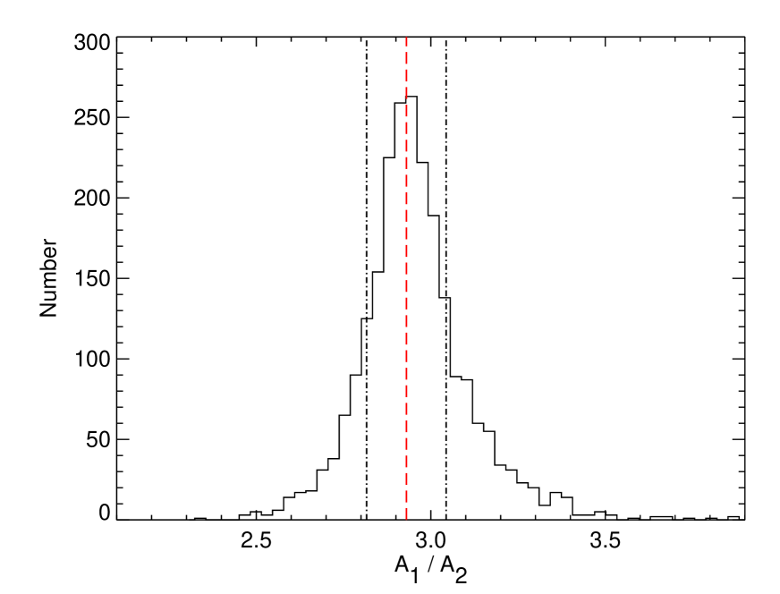
Figure 2: Histogram of the measured amplitude ratios of the [O iii] doublet for our final sample of QSOs. The weighted mean, shown as long-dashed line, corresponds to 2.933$\pm$0.002. The vertical dashed-dotted lines presents the weighted standard deviation of the measured values.

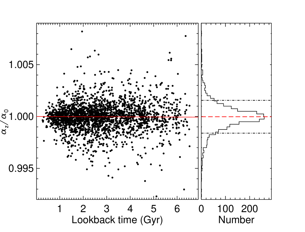
Figure 3: Left: the values of fine-structure constant compared to its laboratory value, $\alpha_{z}/\alpha_{0}$, vs lookback time. The red solid line presents the best fitted line with a slope of $-(0.9\pm 1.1)\times 10^{-5}$ and the intercept of $\alpha_{z}/\alpha_{0}-1$ = $(0.1\pm 1.1)\times 10^{-5}$. Right: the histogram of $\alpha_{z}/\alpha_{0}$. The long-dashed line presents the weighted mean ($\alpha_{z}/\alpha_{0}-1$ = $-2.1\times 10^{-5}$ ) and the dashed-dotted lines present the 2$\sigma$ range ($\sigma=0.00079$) where $\sigma$ is the weighted standard deviation.

The collection of above cuts defines our ”final” sample of 2347 QSOs. We will present $\Delta\alpha/\alpha$ measurements for this sample based on a cross correlation analysis.

2.5 Fe ii emission lines

Fe ii $\lambda$4923 and Fe ii $\lambda$5018 are two Fe ii emission lines that are sometimes seen in the spectra of QSOs in the vicinity of O iii lines. Such a close emission line can influence our measurements as they can distort the shape of the O iii emission lines. However, as predicted by Bahcall et al. (2004) KS test ensures such contamination are not sever in our sample. Inspecting dozens of randomly chosen spectra from our final sample, we did not find any of the QSOs having the above Fe ii emissions. We further stacked spectra of all QSOs in our final sample and did not detect any of these Fe ii emissions in the stacked spectrum. Therefore, such Fe ii emissions will have negligible effect in our $\Delta\alpha/\alpha$ measurements and can not bias our results.

Even though we have used Gaussian fits to define our sample from the full SDSS data set, we use cross-correlation techniques (described below) to measure $\Delta\alpha/\alpha$.

3 cross-correlation analysis for $\Delta\alpha/\alpha$ measurements

The main step in measuring $\alpha$ from a QSO spectrum is to estimate $\Delta\lambda_{{\mathrm{O\,\mathsc{iii}}}}$, the wavelength difference between the two O iii doublet emissions. By further comparison of $\Delta\lambda_{{\mathrm{O\,\mathsc{iii}}}}$ and its laboratory value, 47.9320 Å, we will express one $\Delta\alpha/\alpha$ for each QSO. Cross-correlation analysis has been frequently used for estimating the velocity offset between similar spectral features in the literature (See Wendt & Molaro, 2011; Agafonova et al., 2011; Rahmani et al., 2012, 2013, for examples). Here, we elaborate a cross-correlation analysis to estimate $\Delta\lambda$. To do so we shift each spectrum to the rest frame of the QSO and convert the scales from wavelength to velocity. We then rebin the spectra into new pixel arrays of sizes 10 km s^-1 using a cubic spline interpolation. Finally we perform a cross-correlation analysis between the two O iii emissions which is expressed as following

$$h(V)=(f\star g)(V)=\int_{-\infty}^{\infty}f(v)g(V+v)\,\mathrm{d}v$$ (1)

where $f(v)$ and $g(v)$ correspond to the O iii emission lines which are functions of velocity, $v$, and $h(V)$ is the cross-correlation function where $V$ is the shift. The function $h(V)$ peaks at a velocity, $V_{0}$, where the two O iii doublet profiles best match. We estimate the $V_{0}$ as the peak of a Gaussian function fitted to $h(V)$. The value of fine structure constant at the redshift of the QSO, $\alpha(z)$, can then be estimated as

$$\Delta\alpha/\alpha\equiv\frac{\alpha(z)}{\alpha(0)}-1=\sqrt{1+\frac{V_{0}}{2c\Lambda_{0}^{2}}}-1,~{}~{}~{}~{}~{}\Lambda_{0}=\sqrt{\frac{\lambda_{2}-\lambda_{1}}{\lambda_{2}+\lambda_{1}}}$$ (2)

where $c$ is the speed of light and $\lambda_{1}$ and $\lambda_{2}$ are the laboratory wavelengths of the O iii doublet emission lines. Hence by measuring the $V_{0}$ we directly estimate a $\Delta\alpha/\alpha$ based on each QSO spectrum. We further follow a Monte Carlo simulation to associate a statistical error to each measured $\Delta\alpha/\alpha$. To do this we first generate 100 random realizations of our original QSO spectrum using its error spectrum. We then calculate a $\Delta\alpha/\alpha$ for each of the realized spectra following exactly the same procedure as that of the original spectrum. Finally we calculate the standard deviation of these 100 estimated $\Delta\alpha/\alpha$ and quote it as 1$\sigma$ error of $\Delta\alpha/\alpha$.

The most important step in estimating a $\Delta\alpha/\alpha$ from a QSO spectrum is measuring $V_{0}$. Any systematic error in our cross-correlation analysis can leave biases in our results and lead to unreliable conclusions. Hence it becomes utmost important to check our cross-correlation against any kind of systematic error. To do so we perform a simulation analysis as following: (1) we first measure the velocity shift $\rm v_{0}$ for a randomly chosen QSO. (2) We then apply a velocity shift, $\rm v_{applied}$, to this spectrum and generate 100 realization spectra from this shifted spectrum using its error spectrum. (3) Making use of our cross-correlation routine we measure the velocity shift for each of the 100 realizations to obtain the mean shift of $\rm v_{measured}$. (4) Finally we repeat such an exercise for a sample of applied shifts in the range of $-$50 – 50 km s^-1. Fig. 1 presents the results of this analysis. Clearly the residual differences between the applied and the measured shifts are randomly distributed around zero with a scatter of smaller than tenth of a pixel size. As a result we exclude the possibility that our final values of $\alpha$ is affected by some systematics related to our procedure of measuring shifts.

Table 1: $\Delta\alpha/\alpha$ for various sub-samples of our final sample of QSOs.

Sub-sample†	Sample size	$\Delta\alpha/\alpha$ (10-5)
		weighted mean	simple mean⋆
$z<0.21$	1164	$-2.4\pm 2.1$	$-0.6\pm 1.7$
$z>0.21$	1164	$-1.7\pm 2.6$	$-1.4\pm 2.6$
$\sigma<3.4$ Å	1164	$-2.2\pm 2.2$	$-1.7\pm 1.7$
$\sigma>3.4$ Å	1164	$-2.0\pm 2.7$	$+1.7\pm 2.6$
SNR $<38.5$	1164	$-12.4\pm 3.8$	$-6.5\pm 3.1$
SNR $>38.5$	1164	$+0.3\pm 1.8$	$+0.5\pm 1.5$

^† All sub-samples are made based on the median of the given parameters in this column that are standing for $z$ of the QSO, best fitted $\sigma$ to O iii profile, and the SNR of O iii $\lambda$4959.

^⋆ Simple mean after 2$\sigma$ clipping.

4 results

In this section we summarize the results we get based on the analysis of our final QSO sample. Fig. 2 presents the distribution of the amplitude ratios of the two O iii doublet lines, $A_{2}/A_{1}$. The distribution has a mean of 2.933$\pm$0.002 which is in agreement with its best theoretically estimated value, 2.92, from National Institute of Standards and Technology (NIST) Atomic Spectra Database (Wiese et al., 1996). We would like to recall that this ratio is calculated based on our best fitted Gaussian profiles to O iii doublets. Such an agreement shows that our profile fitting procedure works very well. This is an important issue as the majority of the filters we have defined are built based on the Gaussian profile fitting.

Fig. 3 in its left panel presents our measured $\alpha(z)/\alpha(0)$ vs the lookback time. We have estimated the lookback time based on a standard $\Lambda$CDM background cosmology (Hinshaw et al., 2009) for the redshift of the QSOs. Our best fitted line to these points shows a slope of $(-0.9\pm 1.1)\times 10^{-5}$ and an intercept of $\Delta\alpha/\alpha$ = $(0.1\pm 1.1)\times 10^{-5}$ that are consistent with a no variation in fine-structure constant over last 7 Gyr. The histogram of estimated $\alpha(z)/\alpha(0)$ is shown in the right panel of Fig. 3. We find a weighted mean of $-(2.1\pm 1.6)\times 10^{-5}$ with a weighted standard deviation of 0.00079 for our measured $\Delta\alpha/\alpha$. The reduced $\chi^{2}$ for the weighted mean is 1.1 which shows the quoted error is acceptable. However, we also estimate a simple mean after rejecting outliers by a 2$\sigma$ clipping to get $\Delta\alpha/\alpha$= $-(1.9\pm 1.5)\times 10^{-5}$ with a standard deviation of $\sigma=0.00061$. The estimated weighted mean and simple mean are consistent with each other and with a no variation in the fine-structure constant within 2$\sigma$ errors. Furthermore, the evaluated weighted and standard errors are very much consistent which shows our estimated errors for individual $\Delta\alpha/\alpha$ are realistic. Clearly these measurements provide a substantial improvement to $\Delta\alpha/\alpha$ = $+(1.2\pm 0.7)\times 10^{-4}$ found by Bahcall et al. (2004).

One of the main issues in $\Delta\alpha/\alpha$ measurements is the wavelength stability. Fitting sky and arc lines for each fiber to find the wavelength solution has led to a quite good spectroscopic wavelength calibration in SDSS DR7 and later releases. The typical wavelength calibration error reaches 2 km s^-1 and can be still less in the red part of the spectrograph (Abazajian et al., 2009). By inserting a $V_{0}=2$ km s^-1 in Eq. 2 we convert such an error to ($\Delta\alpha/\alpha$)_cal = $3\times 10^{-4}$. The typical statistical error of $\Delta\alpha/\alpha$ measurements in our study is $\sim$ $10\times 10^{-4}$, which is 3 times larger than ($\Delta\alpha/\alpha$)_cal. In addition, we expect such calibration errors act randomly over a large sample of objects. We further notice that the two spectrograph of SDSS disperse the incoming light on two CCDs called blue and red where the former covers from 3900–6100 Å and the latter from 5900–9100 Å. Hence, a wavelength range of 5900–6100 Å of each object is covered by two spectrograph. Such an overlap with two possible different wavelength solutions in the edges of the two CCDs can impact our results. To check such an effect we exclude those QSOs having their O iii emissions in the above mentioned range from our final sample of QSOs. However, for the remaining (1983) QSOs we find $\Delta\alpha/\alpha$ = $-(1.7\pm 1.7)\times 10^{-5}$ for the weighted mean and $\Delta\alpha/\alpha$ = $-(2.1\pm 1.6)\times 10^{-5}$ for the simple mean after 2$\sigma$ clipping which are consistent with the results we obtained from our final sample of QSOs. Therefore, our results are not affected by the ”possible” systematics due to the different wavelength solutions in the overlapping regions of the two CCDs.

In Table 1 we have further explored the value of $\Delta\alpha/\alpha$ for some more sub-samples of our final sample of QSOs. We have divided our final sample of QSOs into two parts based on the median values of respectively $z$ of the QSOs, $\sigma$ of the best fitted Gaussian to O iii lines, and the SNR of the total flux of the O iii $\lambda$4959 lines. We present both the weighted mean and the simple mean after 2$\sigma$ clipping for all sub-samples. Interestingly there exists a reasonable match between the two estimated errors for each sub-sample. This is a signature for the correct estimate of the error of individual $\Delta\alpha/\alpha$ measurements. The low SNR sub-sample is the only case that is consistent with more than 2$\sigma$ variation of $\alpha$ while having the largest measured error as well. Other sub-samples are always consistent with a stable $\alpha$ with no variation. As expected better constraints are obtained in high SNR and narrow albeit resolved emission lines sub-samples.

5 Conclusion

We have made use of an appropriately chosen sub-sample of QSOs in SDSS DR8 to constrain the possible variation of fine-structure constant by using the O iii $\lambda\lambda$ 4959,5007 nebular emission lines. Our final sample of QSOs consists of 2347 objects. This is the largest sample of objects yet used for constraining the variation of constants. We find $\Delta\alpha/\alpha$ = $-(2.1\pm 1.6)\times 10^{-5}$ at the mean redshift of $z\sim 0.2$. This is consistent with a no variation of $\alpha$ over last 7 Gyr with an accuracy of 10 part in million. This is roughly a factor four improvement compared to the existing measurements based on O iii doublets (Bahcall et al., 2004). However, this constraint is an order of magnitude weaker than those obtained from MM method (Murphy et al., 2003; Srianand et al., 2007). However, because of the large sample of objects and the simplicity of the method our result is much less affected by the systematic errors due to inhomogeneities in the absorbing medium and wavelength calibration errors. Furthermore, we find that our estimated $\Delta\alpha/\alpha$ is fairly consistent in different sub-samples of our main sample of QSOs. As a byproduct of our analysis, we estimated the amplitude ratio of O iii doublet to be 2.933$\pm$0.002 which is in an excellent agreement with its theoretically predicted value, 2.92, from NIST.

Bahcall et al. (2004) had analysed the same O iii doublets from 165 QSOs chosen from SDSS DR1 to find $\Delta\alpha/\alpha$ = $+(1.2\pm 0.7)\times 10^{-4}$. Having a sample that is $\sim$ 14 times larger than that of Bahcall et al. (2004), one expects to reach an accuracy of $\sim 0.7\times 10^{-4}/14^{0.5}=1.9\times 10^{-5}$. This is very close to what we have achieved in our current study. This also illustrate that a 100 fold increase in QSO spectra (i.e. $\sim 10^{5}$) is required to reach the sensitivity of one parts per million in $\Delta\alpha/\alpha$ using O iii doublets.

References

- Abazajian et al. (2009) Abazajian, K. N., Adelman-McCarthy, J. K., Agüeros, M. A., et al., 2009, ApJS, 182, 543
- Agafonova et al. (2011) Agafonova, I. I., Molaro, P., Levshakov, S. A., & Hou, J. L., 2011, A&A, 529, A28+
- Aihara et al. (2011) Aihara, H., Allende Prieto, C., An, D., et al., 2011, ApJS, 193, 29
- Bahcall & Schmidt (1967) Bahcall, J. N. & Schmidt, M., 1967, Physical Review Letters, 19, 1294
- Bahcall et al. (2004) Bahcall, J. N., Steinhardt, C. L., & Schlegel, D., 2004, ApJ, 600, 520
- Chand et al. (2005) Chand, H., Petitjean, P., Srianand, R., & Aracil, B., 2005, A&A, 430, 47
- Chand et al. (2006) Chand, H., Srianand, R., Petitjean, P., Aracil, B., Quast, R., & Reimers, D., 2006, A&A, 451, 45
- Cowie & Songaila (1995) Cowie, L. L. & Songaila, A., 1995, ApJ, 453, 596
- Dzuba et al. (1999a) Dzuba, V. A., Flambaum, V. V., & Webb, J. K., 1999a, Phys. Rev. A, 59, 230
- Dzuba et al. (1999b) —, 1999b, Physical Review Letters, 82, 888
- Griest et al. (2010) Griest, K., Whitmore, J. B., Wolfe, A. M., Prochaska, J. X., Howk, J. C., & Marcy, G. W., 2010, ApJ, 708, 158
- Guéna et al. (2012) Guéna, J., Abgrall, M., Rovera, D., Rosenbusch, P., Tobar, M. E., Laurent, P., Clairon, A., & Bize, S., 2012, Phys. Rev. Lett., 109, 080801
- Hinshaw et al. (2009) Hinshaw, G., Weiland, J. L., Hill, R. S., et al., 2009, ApJS, 180, 225
- Levshakov (1994) Levshakov, S. A., 1994, MNRAS, 269, 339
- Levshakov et al. (2007) Levshakov, S. A., Molaro, P., Lopez, S., D’Odorico, S., Centurión, M., Bonifacio, P., Agafonova, I. I., & Reimers, D., 2007, A&A, 466, 1077
- Molaro et al. (2013) Molaro, P., Centurión, M., Whitmore, J. B., et al., 2013, A&A, 555, A68
- Murphy et al. (2003) Murphy, M. T., Webb, J. K., & Flambaum, V. V., 2003, MNRAS, 345, 609
- Murphy et al. (2001) Murphy, M. T., Webb, J. K., Flambaum, V. V., Prochaska, J. X., & Wolfe, A. M., 2001, MNRAS, 327, 1237
- Petrov et al. (2006) Petrov, Y., Nazarov, A., Onegin, M., Petrov, V., & Sakhnovsky, E., 2006, Phys. Rev. C, 74
- Quast et al. (2004) Quast, R., Reimers, D., & Levshakov, S. A., 2004, A&A, 415, L7
- Rahmani et al. (2012) Rahmani, H., Srianand, R., Gupta, N., Petitjean, P., Noterdaeme, P., & Vásquez, D. A., 2012, MNRAS, 425, 556
- Rahmani et al. (2013) Rahmani, H., Wendt, M., Srianand, R., et al., 2013, MNRAS, 435, 861
- Rosenband et al. (2008) Rosenband, T., Hume, D., Schmidt, P., et al., 2008, Science, 319, 1808
- Savedoff (1956) Savedoff, M. P., 1956, Nature, 178, 688
- Srianand et al. (2007) Srianand, R., Gupta, N., & Petitjean, P., 2007, MNRAS, 375, 584
- Uzan (2003) Uzan, J.-P., 2003, Reviews of Modern Physics, 75, 403
- Uzan et al. (2011) Uzan, J.-P., Ellis, G. F. R., & Larena, J., 2011, General Relativity and Gravitation, 43, 191
- Varshalovich et al. (1996) Varshalovich, D. A., Panchuk, V. E., & Ivanchik, A. V., 1996, Astronomy Letters, 22, 6
- Varshalovich et al. (2000) Varshalovich, D. A., Potekhin, A. Y., & Ivanchik, A. V., 2000, ArXiv Physics e-prints
- Webb et al. (1999) Webb, J. K., Flambaum, V. V., Churchill, C. W., Drinkwater, M. J., & Barrow, J. D., 1999, Physical Review Letters, 82, 884
- Webb et al. (2011) Webb, J. K., King, J. A., Murphy, M. T., Flambaum, V. V., Carswell, R. F., & Bainbridge, M. B., 2011, Physical Review Letters, 107, 191101
- Wendt & Molaro (2011) Wendt, M. & Molaro, P., 2011, A&A, 526, A96+
- Whitmore et al. (2010) Whitmore, J. B., Murphy, M. T., & Griest, K., 2010, ApJ, 723, 89
- Wiese et al. (1996) Wiese, W. L., Fuhr, J. R., & Deters, T. M., 1996, Atomic transition probabilities of carbon, nitrogen, and oxygen : a critical data compilation
- Wolfe et al. (1976) Wolfe, A. M., Brown, R. L., & Roberts, M. S., 1976, Physical Review Letters, 37, 179