Parallel random coordinate descent method for composite minimization: convergence analysis and error bounds
Abstract
In this paper we consider a parallel version of a randomized (block) coordinate descent method for minimizing the sum of a partially separable smooth convex function and a fully separable non-smooth convex function. Under the assumption of Lipschitz continuity of the gradient of the smooth function, this method has a sublinear convergence rate. Linear convergence rate of the method is obtained for the newly introduced class of generalized error bound functions. We prove that the new class of generalized error bound functions encompasses both global/local error bound functions and smooth strongly convex functions. We also show that the theoretical estimates on the convergence rate depend on the number of blocks chosen randomly and a natural measure of separability of the objective function. Numerical simulations are also provided to confirm our theory.
keywords:
Random coordinate descent method, parallel algorithm, partially separable objective function, convergence rate, Lipschitz gradient, error bound property.1 Introduction
In recent years there has been an ever-increasing interest in the optimization community for algorithms suitable for solving convex optimization problems with a very large number of variables. These problems, known as big data problems, have arisen from more recent fields such as network control [1, 2], machine learning [3] and data mining [4]. An important property of these problems is that they are partially separable, which permits parallel and/or distributed computations in the optimization algorithms that are to be designed for them [1, 5]. This, together with the surge of multi-core machines or clustered parallel computing technology in the past decade, has led to the widespread focus on coordinate descent methods.
State of the art: Coordinate descent methods are methods in which a number of (block) coordinates updates of vector of variables are conducted at each iteration. The reasoning behind this is that coordinate updates for problems with a large number of variables are much simpler than computing a full update, requiring less memory and computational power, and that they can be done independently, making coordinate descent methods more scalable and suitable for distributed and parallel computing hardware. Coordinate descent methods can be divided into two main categories: deterministic and random. In deterministic coordinate descent methods, the (block) coordinates which are to be updated at each iteration are chosen in a cyclic fashion or based on some greedy strategy. For cyclic coordinate search, estimates on the rate of convergence were given recently in [6, 7], while for the greedy coordinate search the convergence rate is given e.g. in [8, 9]. On the other hand, in random coordinate descent methods, the (block) coordinates which are to be updated are chosen randomly based on some probability distribution. In [10], Nesterov presents a random coordinate descent method for smooth convex problems, in which only one coordinate is updated at each iteration. Under some assumption of Lipschitz gradient and strong convexity of the objective function, the algorithm in [10] was proved to have linear convergence in the expected values of the objective function. In [11, 12] a 2-block random coordinate descent method is proposed to solve linearly constrained smooth convex problems. The algorithm from [11, 12] was extended to linearly constrained composite convex minimization in [13]. The results in [10] and [14] were combined in [15, 16], in which the authors propose a randomized coordinate descent method to solve composite convex problems. To our knowledge, the first results on the linear convergence of coordinate descent methods under more relaxed assumptions than smoothness and strong convexity were obtained e.g. in [8, 17]. In particular, linear convergence of these methods is proved under some local error bound property, which is more general than the assumption of Lipschitz gradient and strong convexity as required in [10, 11, 12, 13, 15]. However, the authors in [8, 17] were able to show linear convergence only locally. Finally, very few results were known in the literature on distributed and parallel implementations of coordinate descent methods. Recently, a more thorough investigation regarding the separability of the objective function and ways in which the convergence can be accelerated through parallelization was undertaken in [12, 1, 18, 19], where it is shown that speedup can be achieved through this approach. Several other papers on parallel coordinate descent methods have appeared around the time this paper was finalized [20, 11, 5, 21].
Motivation: Despite widespread use of coordinate descent methods for solving large convex problems, there are some aspects that have not been fully studied. In particular, in practical applications, the assumption of Lipschitz gradient and strong convexity is restrictive and the main interest is in finding larger classes of functions for which we can still prove linear convergence. We are also interested in providing schemes based on parallel and/or distributed computations. Finally, the convergence analysis has been almost exclusively limited to centralized stepsize rules and local convergence results. These represent the main issues that we pursue here.
Contribution: In this paper we consider a parallel version of random (block) coordinate gradient descent method [10, 13, 15] for solving large optimization problems with a convex separable composite objective function, i.e. consisting of the sum of a partially separable smooth function and a fully separable non-smooth function. Our approach allows us to analyze in the same framework several methods: full gradient, serial random coordinate descent and any parallel random coordinate descent method in between. Analysis of coordinate descent methods based on updating in parallel more than one (block) component per iteration was given first in [12, 20, 1] and then further studied e.g. in [18, 19]. We provide a detailed rate analysis for our parallel coordinate descent algorithm under general assumptions on the objective function, e.g. error bound type property, and under more knowledge on the structure of the problem and we prove substantial improvement on the convergence rate w.r.t. the existing results from the literature.. In particular, we show that this algorithm attains linear convergence for problems belonging to a general class, named generalized error bound problems. We establish that our class includes problems with global/local error bound objective functions and implicitly strongly convex functions with some Lipschitz continuity property on the gradient. We also show that the new class of problems that we define in this paper covers many applications in networks. Finally, we establish that the theoretical estimates on the convergence rate depend on the number of blocks chosen randomly and a natural measure of separability of the objective function. In summary, the contributions of this paper include:
(i) We employ a parallel version of coordinate descent method and show that the algorithm has sublinear convergence rate in the expected values of the objective function. For this algorithm, the iterate updates can be done independently and thus it is suitable for parallel and/or distributed computing architectures.
(ii) We introduce a new class of generalized error bound problems for which we show that it encompasses both, problems with global/local error bound functions and smooth strongly convex functions and that it covers many practical applications.
(iii) Under the generalized error bound property, we prove that our parallel random coordinate descent algorithm has a global linear convergence rate.
(iv) We also perform a theoretical identification of which categories of problems and objective functions satisfy the generalized error bound property.
Paper Outline: In Section 2 we present our optimization model and discuss practical applications which can be posed in this framework. In Sections 3 and 4 we analyze the properties of a parallel random coordinate descent algorithm, in particular we establish sublinear convergence rate, under some Lipschitz continuity assumptions. In Section 5 we introduce the class of generalized error bound problems and we prove that the random coordinate descent algorithm has global linear convergence rate under this property. In Section 6 we investigate which classes of optimization problems have an objective function that satisfies the generalized error bound property. In Section 7 we discuss implementation details of the algorithm and compare it with other existing methods. Finally, in Section 8 we present some preliminary numerical tests on constrained lasso problem.
2 Problem formulation
In many big data applications arising from e.g. networks, control and data ranking, we have a system formed from several entities, with a communication graph which indicates the interconnections between entities (e.g. sources and links in network optimization [22], website pages in data ranking [3] or subsystems in control [2]). We denote this bipartite graph as , where , and is an incidence matrix. We also introduce two sets of neighbors and associated to the graph, defined as:
The index sets and , which e.g. in the context of network optimization may represent the set of sources which share the link and the set of links which are used by the source , respectively, describe the local information flow in the graph. We denote the entire vector of variables for the graph as . The vector can be partitioned accordingly in block components , with . In order to easily extract subcomponents from the vector , we consider a partition of the identity matrix , with , such that and matrices , such that , with being the vector containing all the components with . In this paper we address problems arising from such systems, where the objective function can be written in a general form as (for similar models and settings, see [1, 18, 23, 22, 21, 5]):
| (1) |
where and . We denote and . The function is a smooth partially separable convex function, while is fully separable convex non-smooth function. The local information structure imposed by the graph should be considered as part of the problem formulation. We consider the following natural measure of separability of the objective function :
Note that , and the definition of the measure of separability is more general than the one considered in [18] that is defined only in terms of . It is important to note that coordinate gradient descent type methods for solving problem (1) are appropriate only in the case when is relatively small, otherwise incremental type methods [22, 24] should be considered for solving (1). Indeed, difficulties may arise when is the sum of a large number of component functions and is large, since in that case exact computation of the components of gradient (i.e. ) can be either very expensive or impossible due to noise. In conclusion, we assume that the algorithm is employed for problems (1), with relatively small, i.e. .
Throughout this paper, by we denote an optimal solution of problem (1) and by the set of optimal solutions. We define the index indicator function as:
and the set indicator function as:
Also, by we denote the standard Euclidean norm and we introduce an additional norm , where is a positive diagonal matrix. Considering these, we denote by the projection of a point onto a set in the norm :
Furthermore, for simplicity of exposition, we denote by the projection of a point on the optimal set , i.e. . In this paper we consider that the smooth component of (1) satisfies the following assumption:
Assumption 1.
We assume that the functions have Lipschitz continuous gradient with a constant :
| (2) |
Note that our assumption is different from the ones in [10, 1, 13, 18], where the authors consider that the gradient of the function is coordinate-wise Lipschitz continuous, which states the following: if we define the partial gradient , then there exists some constants such that:
| (3) |
As a consequence of Assumption 1 we have that [25]:
| (4) |
Based on Assumption 1 we can show the following distributed variant of the descent lemma, which is central in our derivation of a parallel coordinate descent method and in proving the convergence rate for it.
Lemma 1.
Under Assumption 1 the following inequality holds for the smooth part of the objective function :
| (5) |
where is diagonal with its blocks , , and the remaining blocks are zero.
Proof.
If we sum up (4) for and by the definition of we have that:
| (6) |
Given matrices , note that we can express the first term in the right hand side as:
Note that since is a diagonal matrix we can express the norm as:
From the definition of and , note that is equivalent to . Thus, for the final term of the right hand side of (6) we have that:
and the proof is complete. ∎
Note that the convergence results of this paper hold for any descent lemma in the form (5) and thus the expression of the matrix above can be replaced with any other block-diagonal matrix for which (5) is valid. Based on (3) a similar inequality as in (5) can be derived, but the matrix is replaced in this case with the matrix [18]. These differences in the matrices will lead to different step sizes in the algorithms of our paper and of e.g. [1, 18]. Moreover, from the generalized descent lemma through the norm , the sparsity induced by the graph via the sets and and implicitly via the measure of separability will intervene in the estimates for the convergence rates of the algorithm. A detailed discussion on this issue can be found in Section 7. The following lemma establishes Lipschitz continuity for but in the norm , whose proof can be derived using similar arguments as in [25]:
Lemma 2.
For a function satisfying Assumption 1 the following holds:
| (7) |
2.1 Motivating practical applications
We now present important applications from which the interest for problems of type (1) stems.
Application I: One specific example is the sparse logistic regression problem. This type of problem is often found in data mining or machine learning, see e.g. [26, 27]. In a training set , with , the vectors represent samples, and represent the binary class labels with . The likelihood function for these samples is:
where is the conditional probability and is expressed as:
with being the weight vector. In some applications (see e.g. [27]), we require a bias term (also called as an intercept) in the loss function; therefore, is replaced with . The equality defines a hyperplane in the feature space on which . Also, if and otherwise. Then, the sparse logistic regression can be formulated as the following convex problem:
where is some constant and is the average logistic loss function:
Note that , where denotes the 1-norm, is the separable non-smooth component which promotes the sparsity of the decision variable . If we associate to this problem a bipartite graph where the incidence matrix is defined such that provided that , then the vectors have a certain sparsity according to this graph, i.e. they only have nonzero components in . Therefore, can be written as , where each function is defined as:
It can be easily proven that the objective function in this case satisfies (2) with and (3) with . Furthermore, we have that satisfies (5) with matrix .
Application II: Another classic problem which implies functions with Lipschitz continuous gradient of type (2) is:
| (8) |
where , the sets are convex, and . This problem is also known as the constrained lasso problem [28] and is widely used e.g. in signal processing, fused or generalized lasso and monotone curve estimation [28, 29] or distributed model predictive control [1]. For example, in image restoration, incorporating a priori information (such as box constraints on ) can lead to substantial improvements in the restoration and reconstruction process (see [29] for more details). Note that this problem is a special case of problem (1), with being block separable and with the functions defined as:
where are the nonzero components of row of , corresponding to . In this case, functions satisfy (2) with . Given these constants, we find that in this case satisfies (5) with the matrix . Also, note that functions of type (8) satisfy Lipschitz continuity (3) with , where denotes block column of the matrix .
Application III: A third type of problem which falls under the same category is derived from the following primal formulation:
| (9) | ||||
where and the functions are strongly convex with convexity parameters . This type of problem is often found in network control [2], network optimization or utility maximization [22]. In all these applications matrix is very sparse, i.e. both are small. We formulate the dual problem of (9) as:
where denotes the Lagrange multiplier and is the indicator function for the nonnegative orthant . By denoting by the convex conjugate of the function , the previous problem can be rewritten as:
| (10) |
where is the th block column of . Note that, given the strong convexity of , then the functions have Lipschitz continuous gradient in of type (2) with constants [25]. Now, if the matrix has some sparsity induced by a graph, i.e. the blocks if the corresponding incidence matrix has , which in turn implies that the block columns are sparse according to some index set , then the matrix-vector products depend only on , such that , with . Then, has Lipschitz continuous gradient of type (2) with . For this problem we also have componentwise Lipschitz continuous gradient of type (3) with . Furthermore, we find that in this case satisfies (5) with . Note that there are many applications in distributed control or network optimization where or or both are small. E.g., one particular application that appears in the area of network optimization has the structure (9), where the matrix has column linked block angular form, i.e. the matrix has a block structure of the following form:
One of the standard distributed algorithms to solve network problems is based on a dual decomposition as explained above. In this case, by denoting the convex conjugate of the function , the corresponding problem can be rewritten as:
| (11) |
If we consider the block columns of dimension , then depends on all the coordinates of , i.e. . On the other hand, note that given the structure of , we have that . The reader can easily find many other examples of objective functions where .
3 Parallel random coordinate descent method
In this section we consider a parallel version of the random coordinate descent method [10, 13, 15], which we call P-RCD. Analysis of coordinate descent methods based on updating in parallel more than one (block) component per iteration was given first in [12, 20, 1] and then further studied e.g. in [18, 19]. In particular, such a method and its convergence properties has been analyzed in [1, 18], but under the coordinate-wise Lipschitz assumption (3). Before we discuss the method however, we first need to introduce some concepts. For a function as defined in (1), we introduce the following mapping in norm :
| (12) |
Note that the mapping is a fully separable and strongly convex in w.r.t. to the norm with the constant 1. We denote by the proximal step for function , which is the optimal point of the mapping , i.e.:
| (13) |
The proximal step can also be defined in another way. We define the proximal operator of function as:
We recall an important property of the proximal operator [30]:
| (14) |
Based on this operator, note that we can write:
| (15) |
Given that is generally not differentiable, we denote by a vector belonging to the set of subgradients of . Evidently, in both definitions, the optimality conditions of the resulting problem from which we obtain are the same, i.e.:
| (16) |
It will become evident further on that the optimal solution will play a crucial role in the parallel random coordinate descent method. We now establish some properties which involve the function , the mapping and the proximal step . Given that is strongly convex in and that is an optimal point when minimizing over , we have the following inequality:
| (17) |
Further, since is convex and differentiable and by definition of we get:
| (18) |
In the algorithm that we discuss, at a step , the components of the iterate which are to be updated are dictated by a set of indices which is randomly chosen. Let us denote by the vector whose blocks , with , are identical to those of , while the remaining blocks are zeroed out, i.e. or:
| (19) |
Also, for the separable function , we denote the partial sum and the vector . A random variable is uniquely characterized by the probability density function:
For the random variable , we also define the probability with which a subcomponent can be found in as:
In our algorithm, we consider a uniform sampling of unique coordinates , that make up , i.e. . For a random variable with , we observe that we have a total number of possible values that can take, and with the uniform sampling we have that . Given that is random, we can express as:
For a single index , note that we have a total number of possible sets that can take which will include and therefore the probability that this index is in is:
| (20) |
Remark 1.
We can also consider other ways in which can be chosen. For example, we can have partition sets of , i.e. , that are randomly shuffled. We can choose in a nearly independent manner, i.e. is chosen with a sufficient probability, or we can choose according to an irreducible and aperiodic Markov chain, see e.g. [8, 24]. However, if we employ these strategies for choosing , the proofs for the convergence rate of our algorithm follow similar lines.
Having defined the proximal step as in (13), in the algorithm that follows we generate randomly at step an index set of cardinality . We denote the vector which will be used to update , i.e. in the sense that . Also, by we denote the complement set of , i.e. . Thus, the algorithm consists of the following steps:
Parallel random coordinate descent method
(P-RCD)
1.
Consider an initial point and
2.
For :
2.1
Generate with uniform probability a random set of indices ,
with
2.2
Compute:
Note that the iterate update of (P-RCD) method can also be expressed as:
| (21) |
Note that the right hand sides of the last two equalities contain the same optimization problem whose optimality conditions are:
| (22) |
Clearly, the optimization problem from which we compute the iterate of (P-RCD) is fully separable. Then, it follows that for updating component of we need the following data: and . However, the th diagonal entry and th block component of the gradient can be computed distributively according to the communication graph imposed on the original optimization problem. Therefore, if algorithm (P-RCD) runs on a multi-core machine or as a multi-thread process, it can be observed that component updates can be done distributively and in parallel by each core/thread (see Section 7 for details).
We now establish that method (P-RCD) is a descent method, i.e. for all . From the convexity of and (5) we obtain the following:
| (23) |
With (P-RCD) being a descent method, we can now introduce the following term:
| (24) |
and assume it to be bounded. We also define the random variable comprising the whole history of previous events as:
4 Sublinear convergence for smooth convex minimization
In this section we establish the sublinear convergence rate of method (P-RCD) for problems of type (1) with the objective function satisfying Assumption 1. Our analysis in this section combines the tools developed above with the convergence analysis in [16] for random one block coordinate descent methods. The next lemma provides some property for the uniform sampling with :
Lemma 3.
[18, Lemma 3] Let there be some constants with , and a sampling chosen as described above and define the sum . Then, the expected value of the sum satisfies:
| (25) |
For any vector we consider its counterpart for a sampling taken as described above. Given the previous lemma and by taking into account the separability of the inner product and of the squared norm it follows immediately that:
| (26) | |||
| (27) |
Based on relations (26)–(27), the separability of the function , and the properties of the expectation operator, the following inequalities can be derived (see e.g. [18]):
| (28) | |||
| (29) |
We can now formulate an important relation between the gradient mapping in a point and a point . By the definition of and the convexity of and we have:
Furthermore, from the optimality conditions (16) we obtain:
| (30) |
This property will prove useful in the following theorem, which provides the sublinear convergence rate for method (P-RCD).
Theorem 4.
Proof.
Our proof generalizes the proof of Theorem 1 in [16] from one (block) component update per iterate to the case of (block) component updates, based on uniform sampling and on Assumption 1, and consequently on a different descent lemma. Thus, by taking expectation in (23) w.r.t. conditioned on we get:
| (32) |
Now, if we take and in (29) we get:
| (33) |
From this and (30) we obtain:
| (34) | ||||
Denote . From the definition of we have that:
If we divide both sides of the above inequality by and take expectation, we obtain:
Through this inequality and (34) we arrive at:
After some rearranging of terms we obtain the following inequality:
By applying this inequality repeatedly, taking expectation over and from the fact that is decreasing from (32), we obtain the following:
By rearranging some items and since , we arrive at (31). ∎
We notice that given the choice of we get different results (see Section 7 for a detailed analysis). We also notice that the convergence rate depends on the choice of , so that if the algorithm is implemented on a multi-core machine or cluster, then reflects the available number of cores.
Now, given a suboptimality level and a confidence level , we can establish a total number of iterations which will ensure an -suboptimal solution with probability at least .
Corollary 5.
5 Linear convergence for error bound convex minimization
In this section we prove that, for certain minimization problems, the sublinear convergence rate of (P-RCD) from the previous section can be improved to a linear convergence rate. In particular, we prove that under additional assumptions on the objective function, which are often satisfied in practical applications (e.g. the dual of a linearly constrained smooth convex problem or control problem), we have a generalized error bound property for our problem. In these settings we analyze the convergence behavior of algorithm (P-RCD) for which we are able to provide global linear convergence rate, as opposed to the results in [17, 8] where only local linear convergence was derived for deterministic descent methods or the results in [31] where global linear convergence is proved for a gradient method but applied only to problems where is the set indicator function of a polyhedron.
5.1 Linear convergence in the strongly convex case
We assume that the function is additionally strongly convex in the norm with a constant , i.e.:
| (37) |
and since the function has Lipschitz continuous gradient in the the norm with constant , then it automatically holds that . Since is strongly convex function, it follows that optimization problem (1) has a unique optimal point . The following theorem provides the convergence rate of algorithm (P-RCD) when satisfies (37) and its proof follows the lines of the proof in [14].
Theorem 6.
Proof.
If we subtract from both sides of inequality (33) we have that:
| (39) |
From the definition of in (12), of in (13) and from the strong convexity (37) we have that:
We now consider of the form for and since the functions above are convex, then we have that:
| (40) |
Now, since is strongly convex, it satisfies (37) and also the following inequality for any and (see e.g. [25]):
In this inequality, if we take , , and considering that is also convex, we get that:
By replacing this inequality in (40) we get the following:
Now, we can choose a feasible , and therefore we get:
From this and (39) we obtain:
| (41) | ||||
where we note that . Now if we denote , then by taking expectation over in (41) we arrive at:
and linear convergence is proved. ∎
5.2 Linear convergence in the generalized error bound property case
We introduce the proximal gradient mapping of function :
| (42) |
Clearly, a point is an optimal solution of problem (1) if and only if . In the next definition we introduce the Generalized Error Bounded Property (GEBP):
Definition 7.
Problem (1) has the generalized error bound property (GEBP) w.r.t. the norm if there exist two nonnegative constants and such that the composite objective function satisfies the relation (we use ):
| (43) |
Note that the class of functions introduced in (43) includes other known categories of functions. For example, functions composed of a strongly convex function with a convex constant w.r.t. the norm and a general convex function satisfy our definition (43) with and , see Section 6 for more details.
Next, we prove that on optimization problems having the (GEBP) property (43) our algorithm (P-RCD) still has global linear convergence. Our analysis will employ ideas from the convergence proof of deterministic descent methods in [8]. However, the random nature of our method and the the nonsmooth property of the objective function requires a new approach. For example, the typical proof for linear convergence of gradient descent type methods for solving convex problems with an error bound like property is based on deriving an inequality of the form (see e.g. [17, 8, 31]). Under our settings, we cannot derive this type of inequality but instead we obtain a weaker inequality, where we replace with another term and which still allows us to prove linear convergence. We start with the following lemma which shows an important property of algorithm (P-RCD) when it is applied to problems having generalized error bound objective function:
Lemma 8.
Proof.
For the iteration defined by algorithm (P-RCD) we have:
Through this equality and (43) we have that:
| (45) |
and the proof is complete. ∎
Remark 2.
Note that if the iterates of an algorithm satisfy the following relation:
see e.g. the case of the full gradient method [25], then we have:
| (46) |
where .
Let us now note that given the separability of function , then for any vector if we consider their counterparts and for a sampling taken as described above the expected value satisfies:
| (47) | ||||
Furthermore, considering that , then from (44) we obtain:
| (48) |
where . We now need to express explicitly, where is generated by (P-RCD). Note that . As a result:
| (49) |
The following lemma establishes an important upper bound for .
Lemma 9.
Proof.
Taking and in (5) we get:
By adding and substracting in both sides of this inequality and by taking expectation in both sides we obtain (50). Recall the iterate update (21):
Given that is optimal for the problem above and if we take a vector , with , we have that:
Further, if we rearrange the terms and through the convexity of we obtain:
If we divide this inequality by and let we have that:
By adding in both sides of this inequality and observing that:
we obtain (51). ∎
Additionally, note that by applying expectation in to we get:
| (52) | ||||
The following theorem, which is the main result of this section, proves the linear convergence rate for the algorithm (P-RCD) on optimization problems having the generalized error bound property (43).
Theorem 10.
Proof.
We first need to establish an upper bound for . By the definition of and its convexity we have that:
By taking expectation in both sides of the previous inequality we have:
| (54) |
From (24) we have that and derive the following:
where the last step comes from Jensen’s inequality. Thus, (54) becomes:
| (55) |
where . We now explicitly express the second term in the right hand side of the above inequality:
So, by replacing it in (55) and through (49) we get:
| (56) | ||||
By taking and in (5) we obtain:
By rearranging this inequality, we obtain:
Through this and by rearranging terms in (56), we obtain:
| (57) | ||||
Furthermore, from (48) we obtain:
| (58) | ||||
Through the convexity of we have:
and by rearranging it we obtain:
From this and the optimality condition (16) and by replacing in (58) we obtain:
| (59) | ||||
Furthermore, by rearranging some terms and through the Cauchy-Schwartz inequality we obtain:
Now, recall that:
Thus, from this and (48) we get:
By replacing this in (59) we obtain:
| (60) |
From (51) we have:
Now, through this and by rearranging some terms in (60) we obtain:
Furthermore, from (50) we obtain:
By rearranging this inequality, we obtain:
| (61) |
We denote and define . By taking expectation over in (61) we arrive at:
and linear convergence is proved. ∎
Note that we have obtained global linear convergence for our distributed random coordinate descent method on the general class of problems satisfying the generalized error bound property (GEBP) given in (43), as opposed to the results in [8, 17] where the authors only show local linear convergence for deterministic coordinate descent methods applied to local error bound functions, i.e. for all , where is an iterate after which some error bound condition of the form is implicitly satisfied. In [31] global linear convergence is also proved for the full gradient method but applied only to problems having the error bound property where is the set indicator function of a polyhedron. Further, our results are more general than the ones in [10, 11, 12, 1, 13, 18], where the authors prove linear convergence for the more restricted class of problems having smooth and strongly convex objective function. Moreover, our proof for convergence is different from those in these papers.
We now establish the number of iterations which will ensure a -suboptimal solution with probability at least . In order to do so, we first recall that for constants and such that and we have:
| (62) |
6 Conditions for generalized error bound functions
In this section we investigate under which conditions a function satisfying Assumption 1 has the generalized error bound property defined in (43) (see Definition 7).
6.1 Case 1: strongly convex and convex
We first show that if satisfies Assumption 1 and additionally is also strongly convex, while is a general convex function, then has the generalized error bound property defined in (43). Note that a similar result was proved in [8]. For completeness, we also give the proof. We consider to be strongly convex with constant w.r.t. the norm , i.e.:
| (64) |
If is strongly convex w.r.t. the norm , with convexity parameter , then we can redefine and , so that all the above assumptions hold for this new pair of functions.
By Fermat’s rule [30] we have that is also the solution of the following problem:
and since is optimal we get:
Since is strongly convex, then is a singleton and by taking we obtain:
On the other hand from the optimality conditions for and convexity of we get:
By adding up the above two inequalities we obtain:
Now, from strong convexity (64) and Lipschitz continuity (7) we get:
Dividing now both sides of this inequality by , we obtain:
i.e. and in the Definition 7 of generalized error bound functions.
6.2 Case 2: indicator function of a polyhedral set
Another important category of problems (1) that we consider has the following objective function:
| (65) |
where is a smooth convex function, is a constant matrix upon which we make no assumptions and is the indicator function of the polyhedral set . Note that an objective function with the structure in the form (65) appears in many applications, see e.g. the dual problem (10) obtained from the primal formulation (9) given in Section 2.1. Now, for proving the generalized error bound property, we require that satisfies the following assumption:
Assumption 2.
For problem (65), functions under which the set is bounded include e.g. continuously differentiable coercive functions [32]. Also, if (65) is a dual formulation of a primal problem (9) for which the Slater condition holds, then by Theorem 1 of [33] we have that the set of optimal Lagrange multipliers, i.e. in this case, is compact. Also, for we only assume that is a polyhedron (possibly unbounded).
Our approach for proving the generalized error bound property is in a way similar to the one in [17, 8, 31]. However, our results are more general in the sense that they hold globally, while in [17, 8] the authors prove their results only locally and in the sense that we allow the constraints set to be an unbounded polyhedron as opposed to the recent results in [31] where the authors show an error bound like property only for bounded polyhedra or for the entire space . This extension is very important since it allows us e.g. to tackle the dual formulation of a primal problem (9) in which is the nonnegative orthant and which appears in many practical applications. Last but not least important is that our error bound definition and gradient mapping introduced in this paper is more general than the one used in the standard analysis of the classical error bound property (see e.g. [17, 8, 31]), as we can see from the following example:
Example 6.12.
Let us consider the following quadratic problem: . We can easily see that and thus this example satisfies Assumption 2. Clearly, for this example the generalized error bound property (43) holds with e.g. . However, there is no finite constant satisfying the classical error bound property [17, 8, 31]: for all (we can see this by taking in the previous inequality).
By definition, given that is a set indicator function, we observe that the gradient mapping of can be expressed in this case as:
and also note that is an optimal solution of (65) and of (1) if and only if . The following lemma establishes the Lipschitz continuity of :
Lemma 6.13.
For a function whose smooth component satisfies Assumption 1, we have that
| (66) |
Proof 6.14.
By definition of we have that:
and the proof is complete.
The following lemma introduces an important property for the operator .
Lemma 6.15.
Given a convex set , its projection operator satisfies:
| (67) |
Proof 6.16.
The following lemma establishes an important property between and .
Lemma 6.17.
Given a function that satisfies (7) and a convex set , then the following inequality holds:
Proof 6.18.
Denote , then by replacing and in Lemma 6.15 we obtain the following inequality:
Through the definition of the projected gradient mapping, this inequality can be rewritten as:
If we further elaborate the inner product we obtain:
| (69) | ||||
By adding two copies of (69) with and interchanged we have:
From this inequality, through Cauchy-Schwartz and (7) we arrive at:
and the proof is complete.
Lemma 6.19.
Proof 6.20.
Given that as defined in problem (65) is a convex function, then for any two optimal solutions we obtain:
which by the definition of is equivalent to:
If we substract in both sides and by the strong convexity of we have that . Thus, is unique. From this, it is straightforward to see that is constant for all .
Consider now a point and denote by the projection of the point onto the set , as defined in Lemma 6.19, and by its projection onto the optimal set , i.e. . Given the set , the distance to the optimal set can be decomposed as:
Given this inequality, the outline for proving the generalized error bound property (GEBP) from (43) in this case is to obtain appropriate upper bounds for and . In the sequel we introduce lemmas for establishing bounds for these two terms.
Lemma 6.21.
Under Assumption 2, there exists a constant such that:
Proof 6.22.
Corollary 2.2 in [34] states that if we have the following two sets of constraints:
| (70) | |||
| (71) |
then there exists a finite constant such that for a point which satisfies the first set of constraints and a point which satisfies the second one we have:
| (72) |
Furthermore, is only dependent on the matrices and (see [34] for more details). Given that is polyhedral, we can express it as . Thus, for , we can take , in (70), and , in (71) such that:
| (73) | |||
| (74) |
Evidently, a point is feasible for (73). Consider now a point feasible for (74). Therefore, from (72) there exists a constant such that:
Furthermore, from the definition of we get:
| (75) |
From the strong convexity of we have the following property:
for all . From this inequality and Lemma 6.17 we obtain:
Since , it is well known that . Thus, from this and (75) we get:
and the proof is complete.
Note that, if in (65) we have , then by definition we have that , and thus the term . In such a case, also note that and through the previous lemma, in which we established an upper bound for , we can prove outright the error bound property (43) with and . If , the following two lemmas are introduced to investigate the distance between a point and a solution set of a linear programming problem and then to establish a bound for .
Lemma 6.23.
Consider an LP on a nonempty polyhedral set :
| (76) |
and assume that the optimal set is nonempty, convex and bounded. Let be the projection of a point on the optimal set . For this problem we have that:
| (77) |
where is any closed convex set satisfying and depends on and .
Proof 6.24.
Because the solution set is nonempty, convex and bounded, then the linear program (76) is equivalent to the following problem:
and as a result, the linear program (76) is solvable. Now, by the duality theorem of linear programming, the dual problem of (76):
| (78) |
is well defined, solvable and strong duality holds, where is the dual feasible set. For any pair of primal-dual feasible points for problems (76) and (78), we have a corresponding pair of optimal solutions . By the solvability of (76) we have from Theorem 2 of [34], that there exists a constant depending on and such that we have the bound:
Lemma 6.25.
Proof 6.26.
By Lemma 6.19, we have that for all . As a result, the following optimization problem:
has the same solution set as problem (65), due to the fact that . Since is a constant, then we can formulate the equivalent problem:
Note that is constant and under Assumption 2 we have that is convex and bounded. Furthermore, since , then . Considering these details, and by taking , , and in Lemma 6.23 and applying it to the previous problem, we obtain (80).
The next theorem establishes the generalized error bound property for optimization problems in the form (65) having objective functions satisfying Assumption 2.
Theorem 6.27.
Under Assumption 2, the function satisfies the following global generalized error bound property:
| (81) |
where and are two nonnegative constants.
Proof 6.28.
Given that , it is well known that and by Lemma 6.13 we have:
From this inequality and by applying Lemma 6.13, we also have:
From this and Lemma 6.25, we arrive at the following:
| (82) | ||||
Note that since is a bounded set, then we can imply the following upper bound:
Furthermore, since . From this and through the nonexpansive property of the projection operator we obtain:
6.3 Case 3: polyhedral function
We now consider general optimization problems of the form:
| (85) |
where is a polyhedral function. A function is polyhedral if its epigraph, , is a polyhedral set. There are numerous functions which are polyhedral, e.g. with a polyhedral set, , or combinations of these functions. Note that an objective function with the structure (85) appears in many applications (see e.g. the constrained Lasso problem (8) in Section 2.1). Now, for proving the generalized error bound property, we require that satisfies the following assumption.
Assumption 3.
We consider that satisfies Assumption 1. Further, we assume that is strongly convex in with a constant and the optimal set is bounded. We also assume that is bounded above on its domain by a finite value , i.e. for all , and is Lipschitz continuous w.r.t. norm with a constant .
The proof of the generalized error bound property under Assumption 3 is similar to that of [8], but it requires new proof ideas and is done under different assumptions, e.g. that is bounded above on its domain. Boundedness of is in practical applications usually not restrictive. Since is satisfied for any , then problem is equivalent to the following one:
| s.t. |
Consider now an additional variable . Then, the previous problem is equivalent to the following problem:
| (86) | ||||
| s.t. |
Take an optimal pair for problem (86). We now prove that . Consider that is strictly feasible, i.e. . Then, we can imply that is feasible for (86) and the following inequality holds:
which contradicts the fact that is optimal. Thus, it remains that .
The following lemma establishes an equivalence between (86) and another problem:
Proof 6.30.
The proof of this lemma consists of the following two stages: we prove that an optimal point of (86) is an optimal point of (87), and then we prove its converse. Consider now an optimal pair for (86). Since is feasible for (86), we have that and . Recall that . Then, and thus is feasible for (87). Assume now that is not optimal for (87). Then, there exists an optimal pair of (87) such that:
| (88) |
Since is feasible for (87), we have that and inherently . Thus, is feasible and from (88) note that it is optimal for problem (86), which contradicts the fact that is optimal for (86).
Consider now the converse. That is, there exists a pair which is optimal for (87) and is not optimal for (86). Following the same lines as before, note that is feasible for (86). Assume now that is not optimal for (86). Then, there exists a pair such that:
| (89) |
Since is feasible for (86), recall that it is also feasible for (87). Thus, is feasible and optimal for (87), which contradicts the fact that is optimal for (87).
Now, if we denote , then problem (87) can be rewritten as:
| (90) | ||||
| s.t. |
where and . The constraint set for this problem is:
Recall that from Assumption 3 we have that is polyhedral, i.e. there exists a matrix and a vector such that we can express . Thus, we can write the constraint set as:
i.e. is polyhedral. Denote by the set of optimal points of problem (87). Then, from being bounded in accordance with Assumption 3, and the fact that , with continuous function, it can be observed that is also bounded. We now denote , where . Since by Lemma 6.29 we have that problems (86) and (90) are equivalent, then we can apply the theory of the previous subsection to problem (90). That is, we can find two nonnegative constants and such that:
| (91) |
The proximal gradient mapping in this case, is defined as:
where the projection operator is defined in the same manner as . We now show that from the error bound inequality (91) we can derive an error bound inequality for problem (85). From the definitions of , and , we derive the following lower bound for the term on the right-hand side:
| (92) |
Further, note that we can express:
| (93) |
Now, if , then from and the Lipschitz continuity of we have that:
Otherwise, if , we have that:
From these two inequalities we derive the following inequality for :
Therefore, the following upper bound for is established:
| (94) |
We are now ready to present the main result of this section that shows the generalized error bound property for problems in the form (85) under general polyhedral :
Theorem 6.31.
Under Assumption 3, the function satisfies the following global generalized error bound property:
| (95) |
where and .
Proof 6.32.
From the previous discussion, it remains to show that we can find an appropriate upper bound for . Given a point , it can be observed that the gradient of is:
Now, denote . Following the definitions of the projection operator and of , note that is expressed as:
| s.t. |
Furthermore, from the definition of , note that we can also express as:
| s.t. |
Also, given the structure of , consider that . Now, by a simple change of variable, we can define a pair as follows:
| (96) | ||||
| s.t. |
Note that and that we can express and:
From (15) and (42), we can write and recall that can be expressed as:
Thus, we can consider that belongs to a pair which is the optimal solution of the following problem:
| (97) | ||||
Following the same reasoning as in problem (86), note that . Through Fermat’s rule [30] and problem (97), we establish that can also be expressed as:
| (98) | ||||
Therefore, since is optimal for the problem above, we establish the following inequality:
| (99) |
Furthermore, since the pair is optimal for problem (96), we can derive a second inequality:
| (100) | |||
By adding up (99) and (100) we get the following relation:
If we further simplify this inequality we obtain:
Combining the first three terms in the left hand side under the norm and if we multiply both sides by , the inequality becomes:
From this, we derive the following two inequalities:
If we take square root in both of these inequalities, and by applying the triangle inequality to the second, we obtain:
| (101) |
Recall that , and through the Lipschitz continuity of , we have from the first inequality of (101) that:
Furthermore, from the second inequality of (101) we obtain:
From these, we arrive at the following upper bound on :
| (102) | ||||
Finally, from (91), (94) and (102) we obtain the following error bound property for problem (85):
where and .
6.4 Case 4: dual formulation
Consider now the following linearly constrained convex primal problem:
| (103) |
where . In many applications however, its dual formulation is used since the dual structure of the problem is easier, see e.g. applications such as network utility maximization [22] or network control [2]. Now, for proving the generalized error bound property, we require that satisfies the following assumption:
Assumption 4.
We consider that is strongly convex (with constant ) and has Lipschitz continuous gradient (with constant ) w.r.t. the Euclidean norm and there exists such that .
Denoting by the convex conjugate of the function , then from previous assumption it follows that is strongly convex with constant and has Lipschitz gradient with constant (see e.g. [30]). Moreover, from the condition it follows using Gauvin’s theorem that the set of optimal Lagrange multipliers is compact. In conclusion, the previous primal problem is equivalent to the following dual problem:
| (104) |
where is the set indicator function for the nonnegative orthant . From Section 6.2, for , it follows that the dual problem (104) satisfies our generalized error bound property defined in (43) (see Definition 7).
7 Convergence analysis under sparsity conditions
In this section we analyze the distributed implementation and the complexity of algorithm (P-RCD) w.r.t. the sparsity measure and compare it with other complexity estimates from literature.
7.1 Parallel and distributed implementation
Nowadays, many big data applications which appear in the context of networks can be posed as problems of the form (1). Due to the large dimension and the separable structure of these problems, distributed optimization methods have become an appropriate tool for solving such problems. From the iteration of our algorithm (P-RCD) it follows that we can efficiently perform parallel and/or distributed computations. E.g., in the case , we consider that each computer owns the (block) coordinate and the function (provided that it depends on ) and store them locally. Then, our iteration is defined as follows:
where the diagonal block components of the matrix have the expression:
Clearly, for updating we need to compute distributively and . However, can be computed in a distributed fashion since
i.e. node needs to collect the partial gradient from all the functions which depend on the variable (see also [1] for more details on distributed implementation of such an algorithm in the context of network control). We can argue in a similar fashion for computing . Also, for the case where , we can employ other distributed implementations for the algorithm such as the reduce-all approach presented in [5]: if we consider that we have a machine with available cores, then we can distribute the information regarding the functions and block-coordinates per cores, i.e. each core will retain information regarding a multiple number of coordinates and functions . Then, we will require an all-reduced strategy for computing the .
Further, through the norm , which is inherent in , convergence rates from Theorems 4 and 10 depend also on the sparsity induced by the graph via the sets and . As it can be observed, the size of the diagonal elements depends on the values of the Lipschitz constants , with . Clearly these constants are influenced directly by the number of variables that a function depends on. Moreover, depends on the number of individual functions in which block component is found as an argument. For example, let us consider the dual formulation (10) of the primal problem (9). In this case we have . Given that the matrix block is composed of blocks , with , and from the definition of we have the following inequality:
Furthermore, from this inequality and definition of , the diagonal terms of the matrix can be expressed as:
Thus, from the previous inequalities we derive the following upper bound:
In conclusion, our measure of separability for the original problem (1) appears implicitly in the estimates on the convergence rate for our algorithm (P-RCD). On the other hand, the estimate on the convergence rate in [18] depends on the maximum number of connections which a subsystem has, i.e. only on . This shows that our approach is more general, more flexible and thus potentially less conservative, as we will also see in the next section.
7.2 Comparison with other approaches
In this section we compare our convergence rates with those from other existing methods under sparsity conditions. Recall that under Assumption 1 a function satisfies the lemma given in (5):
| (105) |
property which we have employed throughout the paper. The essential element in this relation is the sparsity induced by the sets and , which are reflected in the matrix . Nesterov proves in [10], under the coordinate-wise Lipschitz continuous gradient assumption (3) and without any separability property, the following descent lemma for functions :
| (106) |
where the matrix , with being the Lipschitz constants such that satisfies (3). In [18], under an additional separability assumption on the function , Nesterov’s descent lemma (106) was generalized as follows:
| (107) |
where is defined in Section 2. In order to be able to compare the convergence rates of our method with existing convergence results we assume below that and are of the same magnitude.
Sublinear convergence case: Recall that the sublinear convergence rate of our algorithm (P-RCD), that holds under Assumption 1, is (see Theorem 4):
| (108) |
where . For we obtain a similar convergence rate to that of the random coordinate descent method in [10], i.e. of order , while for we get a similar convergence rate to that of the full composite gradient method of [14]. However, the distances are measured in different norms in these papers. For example, when the comparison of convergence rate in our paper and [14] is reduced to comparing the quantities of [14] with our amount , where is the Lipschitz constant of the smooth component of the objective function, i.e. of , while is defined in a similar fashion as our but in the Euclidean norm, instead of the norm . Let us consider the two extreme cases. First, consider the smooth component of the objective function:
i.e. smooth part is fully separable. Recall that we assume that each individual function is Lipschitz continuous with a constant , as stated in Assumption 1. In this case, it can be easily proven that the Lipschitz constant of is . Thus considering the definition of the matrix in Lemma 1 we have that:
i.e. and our convergence rate is usually better. On the other hand, if we have defined as follows:
then it can be easily proven that and the quantities and would be the same. Thus, we get better rates of convergence when . Finally, we notice that our results are also similar with those of [18], but are obtained under further knowledge regarding the objective function and with a modified analysis. In particular, in [18] two algorithms are proposed: algorithms (PCDM1) and (PCDM2) which explicitly enforces monotonicity. However, in practical large scale applications algorithm (PCDM2) cannot be implemented due to the very large cost per iteration, as the authors also state in their paper. Thus, using a similar reasoning as in [16], we can argue, based on our analysis, that the expected value type of convergence rate given in (31) is better than the one in [18] under certain separability properties as described below. First, the convergence rate of the algorithm in the sublinear case, apart from essentially being of order , depends on the quantity , i.e. implicitly on the stepsizes involved when computing the next iterate , see (21). Thus, in essence, the requirement is to find the smallest values for the diagonal elements of matrix such that Lemma 1 is still valid. To this purpose, we consider the smooth component in (8) in the form . For this problem, consider basic block coordinate, i.e. . Under these considerations, we observe from the table below that our stepsizes are better than those in [18] as increases and . Thus, for certain cases, our analysis can show improvement over the stepsizes in [18] under the same sampling.
| Paper | |
|---|---|
| This paper | |
| [18] | PCDM1: or PCDM2: |
Finally, we proceed to compare the convergence of our algorithm with the algorithms in [18]. Since in practical large scale applications algorithm (PCDM2) in [18] cannot be implemented due to the very large cost per iteration, as the authors also state in their paper, in the sequel we consider algorithm (PCDM1) in [18] under the -uniform sampling, which is similar with our sampling strategy, and for which the authors of [18] were able to derive rate of convergence. In this case, both algorithms (P-RCD) and (PCDM1) have similar costs per iteration. In this setting, (PCDM1) has the following sublinear convergence:
| (109) |
where we define and
| (110) |
Consider that in both algorithms we have that is the smallest term in the two maximums, i.e. and . Let us make a comparison between the two convergence rates, (108) and (109) and note that this comparison comes down to the comparison between the norms and the quantity . From the definitions on the norms we can express:
In conclusion, the sublinear convergence rate of algorithm (P-RCD) is improved under our assumptions, for similarly sized Lipschitz constants and for , i.e. for problems where we have at least a function that depends on a large number of variables (i.e. relatively large) but each variable does not appear in many functions (i.e. relatively small). Note that this scenario was also considered at the beginning of the paper since coordinate gradient descent type methods for solving problem (1) make sense only in the case when is small, otherwise incremental type methods [24] should be considered for solving (1).
Linear convergence case: The authors of [10, 11, 12, 1, 13, 18, 16] also provide linear convergence rate for their algorithms. A straightforward comparison between the convergence rates in this paper and of those in the papers mentioned above cannot be done, due to the fact the linear convergence in all these papers is proved under the more conservative assumption of strong convexity, while the convergence rate of our algorithm (P-RCD) is obtained under the more relaxed assumption of generalized error bound property (43) given in Definition 7. However, we can also consider to be strongly convex with a constant w.r.t. the norm . From Section 6.1 it follows that strongly convex functions are included in our class of generalized error bound functions (43) with and . In this case we can easily prove that we have the following linear convergence of (P-RCD):
| (111) |
where . Note that from (5) it follows that the Lipschitz constant of the gradient is equal to and then combining (5) with (64) we get w.r.t. the norm . In this case, we notice that, given the choice of , we obtain different linear convergence results of order . E.g., for we obtain a similar linear convergence rate to that of the random coordinate descent method in [11, 10, 16, 15], i.e. , while for we get a similar convergence rate to that of the full composite gradient method of [14], i.e . Finally, if we consider to be strongly convex in the norm with a constant and under the same sampling strategy as considered here, then for example the algorithm (PCDM1) in [18] has a convergence rate:
| (112) |
where . Thus, the comparison of convergence rates in this case reduces to the comparison of and . Then, if is sufficiently small and is sufficiently large, we get that and the linear convergence rate (P-RCD) is an improvement over that of [18]. Thus, we found again that under some degree of sparsity (i.e. ) our results are superior to those in [18].
Our convergence results are also more general than the ones in [10, 11, 13, 18, 16], in the sense that we can show linear convergence of algorithm (P-RCD) for larger classes of problems. For example, up to our knowledge the best global convergence rate results known for gradient type methods for solving optimization problems of the form dual formulation of a linearly constrained convex problem (10) or general constrained lasso (8) were of the sublinear form [14, 35]. In this paper we show for the first time global linear convergence rate for random coordinate gradient descent methods for solving this type of problems (8) or (10). Note that for the particular case of least-square problems the authors in [36], using also an error bound like property, were able to show linear convergence for a random coordinate gradient descent method. Our results can be viewed as a generalization of the results from [36] to more general optimization problems. Further, our approach allows us to analyze in the same framework several methods: full gradient, serial coordinate descent and any parallel coordinate descent method in between.
8 Numerical simulations
In this section we present some preliminary numerical results on solving constrained lasso problems in the form (8). The individual constraint sets are box constraints, i.e. . The regularization parameters were chosen uniform for all components, i.e. for all . The numerical experiments were done for two instances of the regularization parameter and . The numerical tests were conducted on a machine with 2 Intel(R) Xeon(R) E5410 quad core CPUs @ 2.33GHz and of RAM. The matrices were randomly generated in Matlab and have a high degree of sparsity (i.e. the measures of partial separability ).
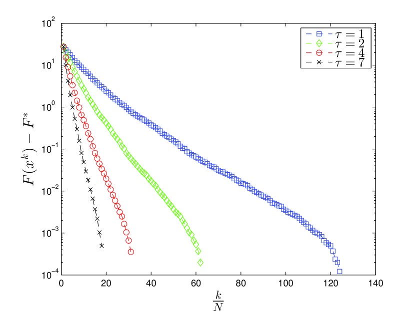
In the first experiment we solve a single randomly generated constrained lasso problem with matrix of dimension and . In this case the two measure of separability have the values: and . The problem was solved on and cores in parallel using MPI for . From Fig. 8.1 and 8.2 we can observe that for each our algorithm needs almost the same number of coordinate updates to solve the problem. On the other hand increasing the number of cores reduces substantially the number of iterations .

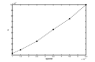
Then, in Fig. 3 for each randomly generated problems with varying sparsity ranging from to and dimension and we plot the average number of iterations. We consider and . We observe that the number of iterations increases once the sparsity decreases.
| 1 | 35 | 38 | 177 | 279 | 2420.107 | |||
| 55 | 52 | 274 | 432 | 2379.622 | ||||
| 64 | 63 | 418 | 605 | 1985.261 | ||||
| 71 | 66 | 364 | 556 | 2422.455 | ||||
| 68 | 69 | 397 | 635 | 2307.750 | ||||
| 31 | 32 | 111 | 193 | 27768.840 | ||||
| 34 | 36 | 128 | 238 | 25918.885 | ||||
| 43 | 41 | 167 | 285 | 25860.573 | ||||
| 41 | 42 | 162 | 280 | 26894.849 | ||||
| 42 | 42 | 161 | 270 | 28405.369 | ||||
| 40 | 38 | 119 | 207 | 287300.02 | ||||
| 34 | 36 | 144 | 235 | 251255.96 | ||||
| 43 | 44 | 109 | 229 | 227031.21 | ||||
| 46 | 43 | 101 | 187 | 273215.09 | ||||
| 51 | 53 | 99 | 182 | 239189.71 | ||||
| 10 | 39 | 42 | 24 | 38 | 4884.610 | |||
| 51 | 52 | 38 | 62 | 4762.226 | ||||
| 64 | 70 | 52 | 85 | 4477.707 | ||||
| 65 | 65 | 57 | 81 | 4909.406 | ||||
| 68 | 68 | 51 | 83 | 4922.320 | ||||
| 34 | 31 | 13 | 28 | 46066.411 | ||||
| 32 | 35 | 16 | 33 | 47770.23 | ||||
| 40 | 46 | 23 | 43 | 45520.275 | ||||
| 42 | 43 | 23 | 43 | 49808.196 | ||||
| 46 | 43 | 22 | 41 | 54370.699 | ||||
| 35 | 37 | 14 | 26 | 449548.04 | ||||
| 41 | 40 | 18 | 33 | 467529.31 | ||||
| 42 | 43 | 22 | 42 | 452739.23 | ||||
| 43 | 44 | 17 | 36 | 426963.31 | ||||
| 48 | 43 | 19 | 39 | 442936.02 |
In the second set of experiments, provided in Table 1, the dimension of matrix ranges as follows: from to and from to . For the resulting problem our objective function satisfies the generalized error bound property (43) given in Definition 7 and in some cases it is even strongly convex. This series of numerical tests were undertaken in order to compare the full number of iterations of the algorithm under the original assumptions considered in [18] and the ones considered for the algorithm in this paper.
In these simulations the algorithms were implemented in a centralized manner, i.e. there is no inter-core transmission of data, with the number of updates per iteration of in each case. In both cases the algorithms were allowed to reach the same optimal value which is presented in the last column and was computed with the serial () random coordinate descent method. The second and third column of the table represent the dimensions of matrix . The fourth column represents the degree of sparsity which dictates that the total number of nonzero elements in the matrix is less than or equal to . The fifth and sixth columns denote the degrees of partial separability and , while the seventh and eighth columns represent the total number of coordinate updates normalized that the algorithms completed. As it can be observed from Table 1, algorithm (P-RCD) outperforms (PCDM1) of [18] even in the case where and are of similar size or equal. Moreover, note that between the problems where is slightly larger than , i.e. where the resulting objective function is strongly convex, and the problems where is slightly smaller than , i.e. where is not strongly convex but satisfies our generalized error bound property (43), the number of iterations of algorithm (P-RCD) is comparable. In conclusion, given that the constrained lasso problems of the form (8) satisfy the generalized error bound property (43), the theoretical result that linear convergence of algorithm (P-RCD) is attained under the generalized error bound property is confirmed also in practice.
References
- [1] I. Necoara and D. Clipici. Efficient parallel coordinate descent algorithm for convex optimization problems with separable constraints: application to distributed mpc. Journal of Process Control, 23(3):243–253, 2013.
- [2] I. Necoara and J.A.K. Suykens. An interior-point lagrangian decomposition method for separable convex optimization. Journal of Optimization Theory and Applications, 143(3):567–588, 2009.
- [3] C.M. Bishop. Pattern Recognition and Machine Learning. Springer-Verlag, 2006.
- [4] I.H. Witten, E. Frank, and M.A. Hall. Data Mining: Practical Machine Learning Tools and Techniques. Elsevier, New York, 2011.
- [5] P. Richtarik and M. Takac. Distributed coordinate descent method for learning with big data. Technical report, Univ. Edinburgh, Oct. 2013.
- [6] A. Beck and L. Tetruashvili. On the convergence of block coordinate descent type methods. SIAM Journal on Optimization, 23(4):2037–2060, 2013.
- [7] M. Hong, X. Wang, M. Razaviyayn, and Z-Q. Luo. Iteration complexity analysis of block coordinate descent methods. Technical report, University of Minnesota, USA, 2013. http://arxiv.org/abs/1310.6957.
- [8] P. Tseng and S. Yun. A coordinate gradient descent method for nonsmooth separable minimization. Mathematical Programming, 117(1–2):387–423, 2009.
- [9] P. Tseng. Convergence of a block coordinate descent method for nondifferentiable minimization. Journal of Optimization Theory and Applications, 109(3):475–494, 2001.
- [10] Y. Nesterov. Efficiency of coordinate descent methods on huge-scale optimization problems. SIAM Journal on Optimization, 22(2):341–362, 2012.
- [11] I. Necoara. Random coordinate descent algorithms for multi-agent convex optimization over networks. IEEE Trans. Automatic Control, 58(8):2001–2012, 2013.
- [12] I. Necoara, Y. Nesterov, and F. Glineur. A random coordinate descent method on large optimization problems with linear constraints. Technical report, University Politehnica Bucharest, July 2011.
- [13] I. Necoara and A. Patrascu. A random coordinate descent algorithm for optimization problems with composite objective function and linear coupled constraints. Computational Optimization and Applications, 57(2):307–337, 2014.
- [14] Y. Nesterov. Gradient methods for minimizing composite objective functions. Mathematical Programming, 140(1):125–161, 2013.
- [15] P. Richtarik and M. Takac. Iteration complexity of randomized block-coordinate descent methods for minimizing a composite function. Mathematical Programming, 144:1–38, 2014.
- [16] Z. Lu and L. Xiao. On the complexity analysis of randomized block-coordinate descent methods. Technical report, 2013. http://arxiv.org/abs/1305-4723.
- [17] Z.Q. Luo and P. Tseng. Error bounds and convergence analysis of feasible descent methods: a general approach. Annals Operations Research, 46(1):157–178, 1993.
- [18] P. Richtarik and M. Takac. Parallel coordinate descent methods for big data optimization. Technical report, Univ. Edinburgh, Dec. 2012.
- [19] Z. Peng, M. Yan, and W. Yin. Parallel and distributed sparse optimization. Technical report, Rice University, USA, 2013.
- [20] J..K Bradley, A. Kyrola, D. Bickson, and C. Guestrin. Parallel coordinate descernt for -regularized loss minimization. ICML, 2011.
- [21] M. Takac, A. Bijral, P. Richtarik, and N. Srebro. Mini-batch primal and dual methods for svms. Technical report, Univ. Edinburgh, March 2013.
- [22] S. Sundhar Ram, A. Nedic, and V.V. Veeravalli. Incremental stochastic subgradient algorithms for convex optimization. SIAM Journal on Optimization, 20(2):691–717, 2009.
- [23] F. Niu, B. Recht, C. Re, and S. Wright. Hogwild!: A lock-free approach to parallelizing stochastic gradient descent. NIPS, 2012.
- [24] M. Wang and D. P. Bertsekas. Incremental constraint projection-proximal methods for nonsmooth convex optimization. Technical report, MIT, July 2013.
- [25] Y. Nesterov. Introductory Lectures on Convex Optimization: A Basic Course. Kluwer, Boston, USA, 2004.
- [26] S. Ryali, K. Supekar, D. A. Abrams, and V. Menone. Sparse logistic regression for whole-brain classification of fmri data. NeuroImage, 51(2):752–764, 2010.
- [27] G.X. Yuan, K.W. Chang, C.J. Hsieh, and C.J. Lin. A comparison of optimization methods and software for large-scale -regularized linear classification. Journal of Machine Learning Research, 11:3183–3234, 2010.
- [28] G.M. James, C. Paulson, and P. Rusmevichientong. The constrained lasso. Technical report, University of Southern California, 2013.
- [29] X. Chen, M. K. Ng, and C. Zhang. Non-lipschitz -regularization and box constrained model for image restoration. IEEE Transactions on Image Processing, 21(12):4709–4721, 2012.
- [30] R.T. Rockafellar and R.J. Wets. Variational Analysis. Springer-Verlag, 1998.
- [31] P.W. Wang and C.J. Lin. Iteration complexity of feasible descent methods for convex optimization. Technical report, National Taiwan University, 2013.
- [32] S. Ma and S. Zhang. An extragradient-based alternating direction method for convex minimization. Technical report, Chinese University of Hong Kong, January 2013.
- [33] O.L. Mangasarian. Computable numerical bounds for lagrange multipliers of stationary points of non-convex differentiable non-linear programs. Operations Research Letters, 4(2):47–48, 1985.
- [34] S. M. Robinson. Bounds for error in the solution set of a perturbed linear program. Linear Algebra and its Applications, 6:69–81, 1973.
- [35] I. Necoara and V. Nedelcu. Rate analysis of inexact dual first order methods: application to dual decomposition. IEEE Transactions on Automatic Control, 59(5):1232–1243, 2014.
- [36] D. Leventhal and A.S. Lewis. Randomized methods for linear constraints: Convergence rates and conditioning. Technical report, Cornell University, 2008. http://arxiv.org/abs/0806.3015.