Systematic and multifactor risk models revisited

Abstract

Systematic and multifactor risk models are revisited via methods which were already successfully developed in signal processing and in automatic control. The results, which bypass the usual criticisms on those risk modeling, are illustrated by several successful computer experiments.

1 Introduction

Systematic, or market, risk is one of the most studied risk models not only in financial engineering, but also in actuarial sciences, in business and corporate management, and in several other domains. It is associated to the beta ($\beta$) coefficient, which is familiar in the investment industry since Sharpe’s capital asset pricing model (CAPM) sharpe1 . The pitfalls and shortcomings of $\beta$ have been detailed by a number of excellent authors. Replacing moreover time-invariant linear regressions by time-varying and/or nonlinear ones does not seem to improve this situation. The model-free standpoint advocated in beta and douai alleviates several of the known deficiencies but unfortunately cannot be extended to multifactor risk models which became also popular after Ross’ arbitrage pricing theory (APT) ross . In order to encompass the univariate and multivariate cases, we propose here a unified definition, with the same advantages, namely a clear-cut mathematical foundation, which

• bypasses clumsy statistical and/or financial assumptions,

• leads to efficient computations.

Our approach is based on the following ingredients:

• As in our previous works fes ; beta ; douai ; agadir we utilize the Cartier-Perrin theorem cartier . It shows that under a mild integrability condition any time series may decomposed as a sum of a mean, or trend, and of quick fluctuations.

• Classic mathematical tools like the Wronski determinants ince .

• We employ recent estimation and identification techniques sira1 ; sira2 , which are stemming from control theory and signal processing where they have been utilized quite successfully.

From a more practical standpoint, our main result is the derivation of two independent $\beta$ coefficients, the first one for the comparison between returns and the second one for the comparison between volatilities. It implies among other consequences that the importance of the popular $\alpha$ coefficient might vanish.

Our paper is organized as follows. After a short review of the Cartier-Perrin theorem, Section 2 details the new mathematical definitions of the coefficients $\alpha$ and $\beta$, and of $\beta$ alone. Section 3 develops the comparison with the classical settings. Computer illustrations are provided in Section 4.

Future publications will be exploiting the above advances in at least three directions:

1. The extension of Section 3.3 to skewness and kurtosis should be straightforward. Our understanding, which would not rely exclusively any more on “Gaussianism”, of the respective behaviors of various assets might therefore be quite enhanced.

2. According to the methods sketched in agadir and in pricing , dynamic portfolio management and option pricing may be achieved by tracking quite independent performances with respect to returns and volatilities.

3. We will relate some instances of systemic risk to the abrupt changes abrupt of some quantities like our new beta coefficients (see fes ; beta ; douai for preliminary results).

2 Theoretical background

2.1 A short review on time series via nonstandard analysis

Take the time interval $[0,1]\subset\mathbb{R}$ and introduce as often in nonstandard analysis the infinitesimal sampling

$${\mathfrak{T}}=\{0=t_{0}<t_{1}<\dots<t_{N}=1\}$$

where $t_{\iota+1}-t_{\iota}$, $0\leq\iota<N$, is infinitesimal, i.e., “very small”. A time series $X(t)$ is a function $X:{\mathfrak{T}}\rightarrow\mathbb{R}$.

The Lebesgue measure on ${\mathfrak{T}}$ is the function $\ell$ defined on ${{\mathfrak{T}}}\backslash\{1\}$ by $\ell(t_{i})=t_{i+1}-t_{i}$. The measure of any interval $[c,d]\subset\mathfrak{I}$, $c\leq d$, is its length $d-c$. The integral over $[c,d]$ of the time series $X(t)$ is the sum

$$\int_{[c,d]}Xd\tau=\sum_{t\in[c,d]}X(t)\ell(t)$$

$X$ is said to be $S$-integrable if, and only if, for any interval $[c,d]$ the integral $\int_{[c,d]}|X|d\tau$ is limited, i.e. not infinitely large, and, if $d-c$ is infinitesimal, also infinitesimal.

$X$ is $S$-continuous at $t_{\iota}\in{\mathfrak{T}}$ if, and only if, $f(t_{\iota})\simeq f(\tau)$ when $t_{\iota}\simeq\tau$. $X$ is said to be almost continuous if, and only if, it is $S$-continuous on ${\mathfrak{T}}\setminus R$, where $R$ is a rare subset. $X$ is Lebesgue integrable if, and only if, it is $S$-integrable and almost continuous.

A time series ${\mathcal{X}}:{\mathfrak{T}}\rightarrow\mathbb{R}$ is said to be quickly fluctuating, or oscillating, if, and only if, it is $S$-integrable and $\int_{A}{\mathcal{X}}d\tau$ is infinitesimal for any quadrable subset.

Let $X:{\mathfrak{T}}\rightarrow\mathbb{R}$ be a $S$-integrable time series. Then, according to the Cartier-Perrin theorem cartier , the additive decomposition

$$\boxed{X(t)=E(X)(t)+X_{\tiny{\rm fluctuat}}(t)}$$ (1)

holds where

• the mean $E(X)(t)$ is Lebesgue integrable,

• $X_{\tiny{\rm fluctuat}}(t)$ is quickly fluctuating.

The decomposition (1) is unique up to an infinitesimal.

Remark 1

Decomposition (1), where $E(X)(t)$ is “smoother” than $X(t)$, provides, to the best of our knowledge, the first complete theoretical justification (see fes ) of the trends in technical analysis (see, e.g., bechu ; kirk ).

2.2 Multivariate factors

Arithmetical average

Assume that $X:{\mathfrak{T}}\rightarrow\mathbb{R}$ is $S$-integrable. Take a quadrable set $A\subseteq{\mathfrak{T}}$ such that $\int_{A}d\tau$ is appreciable, i.e., non-infinitesimal. The arithmetical average of $X$ on $A$, which is written $\text{AV}_{A}(X)$, is defined by

$$\boxed{\text{AV}_{A}(X)=\frac{\int_{A}Xd\tau}{\int_{A}d\tau}}$$

It follows at once from Equation (1) that the difference between $\text{AV}_{A}(X)$ and $\text{AV}_{A}(E(X))$ is infinitesimal, i.e.,

$$\text{AV}_{A}(X)\simeq\text{AV}_{A}(E(X))$$

In practice, $A$ is a time interval $[t-L,t]$, with an appreciable length $L$. Set, if $t\geq L$,

$$\boxed{\overline{X}(L,t)=\text{AV}_{[t-L,t]}(X)=\frac{\int_{t-L}^{t}Xd\tau}{L}\simeq\frac{\int_{t-L}^{t}E(X)d\tau}{L}}$$ (2)

Introduce

$$\overline{X}^{[\nu]}(L,t)=\frac{1}{(\nu-1)!}\int_{t-L}^{t}(t-\tau)^{\nu-1}Xd\tau$$ (3)

It corresponds via the classic Cauchy formula to an iterated integral of order $\nu$ (see, e.g., folland ). Note that $\overline{X}^{[1]}(L,t)=\overline{X}(L,t)$.

2.3 Alpha and betas

Take $n+1$ $S$-integrable time series $Y,X_{1},\dots,X_{n}:{\mathfrak{T}}\rightarrow\mathbb{R}$. Assume, without any loss of generality, that their values at any $t_{\iota}\in{\mathfrak{T}}$ is bounded by a given limited number. Set

$$\boxed{\overline{Y}(L,t)=\alpha(L,t)+\beta_{1}(L,t)\overline{X}_{1}(L,t)+\dots+\beta_{n}(L,t)\overline{X}_{n}(L,t)}$$

$\alpha(L,t)$, $\beta_{i}(L,t)\in\mathbb{R}$, $i=1,\dots,n$, are not yet uniquely determined.

Define the time series $\mathbf{1}:{\mathfrak{T}}\rightarrow\mathbb{R}$, $t_{\iota}\mapsto 1$. Its arithmetical average is always $1$. Equation (3) yields

$$\overline{\mathbf{1}}^{[\nu]}(L,t)=\frac{L^{\nu-1}}{\nu!}$$

Introduce the Wronskian-like determinant (see, e.g., ince )

$$W_{{\mathbf{1}},X_{1},\dots,X_{n}}(L,t)=\begin{vmatrix}1&\overline{X}^{[1]}_{1}(L,t)&\dots&\overline{X}^{[1]}_{n}(L,t)\\ \dots&\dots&\dots&\dots\\ \frac{L^{n}}{(n+1)!}&\overline{X}^{[n+1]}_{1}(L,t)&\dots&\overline{X}^{[n+1]}_{n}(L,t)\end{vmatrix}$$ (4)

$X_{1},\dots,X_{n}$ are said to be $\alpha$-W-independent on $[t-L,t]$ if, and only if, $W_{{\mathbf{1}},X_{1},\dots,X_{n}}(L,t)$ is appreciable.

Introduce the $(n+1)\times(n+2)$ matrix

$${\mathcal{M}}_{Y,{\mathbf{1}},X_{1},\dots,X_{n}}(L,t)=\begin{pmatrix}\overline{Y}^{[1]}(L,t)&1&\overline{X}^{[1]}_{1}(L,t)&\dots&\overline{X}^{[1]}_{n}(L,t)\\ \dots&\dots&\dots&\dots&\dots\\ \overline{Y}^{[n+1]}(L,t)&\frac{L^{n}}{(n+1)!}&\overline{X}^{[n+1]}_{1}(L,t)&\dots&\overline{X}^{[n+1]}_{n}(L,t)\end{pmatrix}$$ (5)

Assume that $X_{1},\dots,X_{n}$ are $\alpha$-W-independent on $[t-L,t]$. Then the matrix (5) is of rank $n+1$. The Cramer rule yields limited values for $\alpha(L,t)$, $\beta_{1}(L,t)$, …, $\beta_{n}(L,t)$ in Equation (2.3):

$$\alpha(L,t)=\frac{\begin{vmatrix}\overline{Y}^{[1]}(L,t)&\overline{X}^{[1]}_{1}(L,t)&\dots&\overline{X}^{[1]}_{n}(L,t)\\ \dots&\dots&\dots&\dots\\ \overline{Y}^{[n+1]}(L,t)&\overline{X}^{[n+1]}_{1}(L,t)&\dots&\overline{X}^{[n+1]}_{n}(L,t)\end{vmatrix}}{W_{{\mathbf{1}},X_{1},\dots,X_{n}}(L,t)}$$

$$\beta_{1}(L,t)=\frac{\begin{vmatrix}1&\overline{Y}^{[1]}(L,t)&\overline{X}^{[1]}_{2}(L,t)&\dots&\overline{X}^{[1]}_{n}(L,t)\\ \dots&\dots&\dots&\dots\\ \frac{L^{n}}{(n+1)!}&\overline{Y}^{[n+1]}(L,t)&\overline{X}^{[n+1]}_{2}(L,t)&\dots&\overline{X}^{[n+1]}_{n}(L,t)\end{vmatrix}}{W_{{\mathbf{1}},X_{1},\dots,X_{n}}(L,t)}$$

…

$$\beta_{n}(L,t)=\frac{\begin{vmatrix}1&\overline{X}^{[1]}_{1}(L,t)&\dots&\overline{X}^{[1]}_{n-1}(L,t)&\overline{Y}^{[1]}(L,t)\\ \dots&\dots&\dots&\dots\\ \frac{L^{n}}{(n+1)!}&\overline{X}^{[n+1]}_{1}(L,t)&\dots&\overline{X}^{[n+1]}_{n-1}(L,t)&\overline{Y}^{[n+1]}(L,t)\end{vmatrix}}{W_{{\mathbf{1}},X_{1},\dots,X_{n}}(L,t)}$$

Remark 2

Replacing in Equation (2.3) the arithmetic averages by the original time series yields

$$Y=\alpha(L,t)+\beta_{1}(L,t)X_{1}+\dots+\beta_{n}(L,t)X_{n}+e_{[t-L,t]}$$

where $\int_{t-L}^{t}e_{[t-L,t]}d\tau$ is infinitesimal.

2.4 Betas alone

Let us drop $\alpha$. Equation (2.3) becomes

$$\overline{Y}(L,t)=\sum_{i=1}^{n}\beta_{i}(L,t)\overline{X}_{i}(L,t)$$ (6)

Determinant (4) is replaced by

$$W_{X_{1},\dots,X_{n}}(L,t)=\begin{vmatrix}\overline{X}^{[1]}_{1}(L,t)&\dots&\overline{X}^{[1]}_{n}(L,t)\\ \dots&\dots&\dots\\ \overline{X}^{[n]}_{1}(L,t)&\dots&\overline{X}^{[n]}_{n}(L,t)\end{vmatrix}$$

$X_{1},\dots,X_{n}$ are said to be W-independent on $[t-L,t]$ if, and only if, $W_{X_{1},\dots,X_{n}}(L,t)$ is appreciable. Matrix (5) is replaced by the $n\times(n+1)$ matrix

$${\mathcal{M}}_{Y,X_{1},\dots,X_{n}}(L,t)=\begin{pmatrix}\overline{Y}^{[1]}(L,t)&\overline{X}^{[1]}_{1}(L,t)&\dots&\overline{X}^{[1]}_{n}(L,t)\\ \dots&\dots&\dots&\dots\\ \overline{Y}^{[n]}(L,t)&\overline{X}^{[n]}_{1}(L,t)&\dots&\overline{X}^{[n]}_{n}(L,t)\end{pmatrix}$$

Assume that $X_{1},\dots,X_{n}$ are W-independent on $[t-L,t]$. Then ${\mathcal{M}}_{Y,X_{1},\dots,X_{n}}(L,t)$ is of rank $n$. Limited values for $\beta_{i}(L,t)$, $i=1,\dots,n$ are again given by the Cramer rule. Although we do not give again the formulae, it goes without saying that these numerical values are in general different from those derived in Sect. 2.3. We do not repeat also Remark 2.

Remark 3

If $n=1$ and $\int_{t-L}^{t}\overline{Y}d\tau\neq 0$,

$$\beta_{1}(L,t)=\frac{\overline{X}_{1}(L,t)}{\overline{Y}(L,t)}=\frac{\int_{t-L}^{t}\overline{X}_{1}d\tau}{\int_{t-L}^{t}\overline{Y}d\tau}$$ (7)

3 Comments

3.1 The model-free standpoint

The length $L$ of the time window $[t-L,t]$ may be chosen quite short, i.e., of a size compatible with what is needed for calculating the trends in fes . Updating the various factors is achieved by letting slide this time window. Let us emphasize that the linearity of the local models (2.3) and (6), which are valid only during a short time interval, does not imply therefore a global time-invariant linearity as assumed in the CAPM and APT settings. This model-free standpoint has already been proved to be quite efficient in control theory.

Remark 4

Equations (2.3) and (6) should not be viewed as time-varying linear relations, since the values of their coefficients depend nonlinearly on $X_{1}$, …, $X_{n}$.

3.2 Reverse formula

Take for simplicity’s sake $n=1$ in Equation (2.3). Then

$$\overline{Y}(L,t)=\alpha+\beta_{1}(L,t)\overline{X}_{1}(L,t)$$

yields, if $\beta_{1}(L,t)\neq 0$,

$$\overline{X}_{1}(L,t)=-\frac{1}{\alpha(L,t)}+\frac{1}{\beta_{1}(L,t)}\overline{Y}(L,t)$$

The same reverse formula would have also been derived from the linear algebra of Section 2.4.

Now, we restrict ourselves for simplicity’s sake to a CAPM-like equation

$$r(t)=\alpha+\beta R(t)+\epsilon(t)$$ (8)

where

• $r(t)$ and $R(t)$ are the values at time $t$ of some returns,

• $\epsilon(t)$ is a zero-mean stochastic processes,

• $\alpha$ and $\beta$ are constant.

As pointed out in tofa , the classic least square techniques utilized with Equation (8) do not lead to the most natural reverse formula.

3.3 Volatility

Today’s situation

Consider again Equation (8). This global linear time-invariant equation leads to usual systematic, or market, risk calculation, i.e, to

$$\text{var}(r)=\beta^{2}\text{var}(R)+\text{var}(\epsilon)$$ (9)

where $\text{var}(\epsilon)$ should be “small” if there is a “good” diversification. It explains

1. why increasing $\beta$ also increases the risk,

2. the importance of generating a “good” $\alpha$ in Equation (8).

If, as emphasized in tofa , Equation (8) does not hold, i.e., there is no global linear time-invariant relationship, Equation (9) is then erroneous. The whole “philosophy” which was built in order to justify the utilization of the CAPM and of its extensions like the APT (see, e.g., bodie ) might therefore break down.

Remark 5

Equation (2) shows that the quick fluctuations do not appear in Equations (2.3) and (6). Those equations are therefore useful for comparing the time evolution of means, i.e., trends, and certainly not for the comparison of the corresponding volatilities.

A remedy

We start by reviewing the definitions of (co)variances and volatility given in douai ; agadir . Take two $S$-integrable time series $X$, $Y$ such that their squares and the squares of $E(X)$ and $E(Y)$ are also $S$-integrable. Then the following property is obvious: $XY$, $E(X)E(Y)$, $E(X)Y_{\tiny{\rm fluctuat}}$, $X_{\tiny{\rm fluctuat}}E(Y)$, $X_{\tiny{\rm fluctuat}}Y_{\tiny{\rm fluctuat}}$ are all $S$-integrable. Assume moreover that $E(X)$ and $E(Y)$ are differentiable in the following sense: there exist two Lebesgue integrable time series $f,g:{\mathfrak{T}}\rightarrow\mathbb{R}$, such that, $\forall\leavevmode\nobreak\ t\in{\mathfrak{T}}$, with the possible exception of a limited number of values of $t$, $E(X)=E(X)(0)+\int_{0}^{t}f(\tau)d\tau$, $E(Y)=E(Y)(0)+\int_{0}^{t}g(\tau)d\tau$. Integrating by parts shows that the products $E(X)Y_{\tiny{\rm fluctuat}}$ and $X_{\tiny{\rm fluctuat}}E(Y)$ are quickly fluctuating.

Remark 6

Let us emphasize that the product $X_{\tiny{\rm fluctuat}}Y_{\tiny{\rm fluctuat}}$ is not necessarily quickly fluctuating.

The following definitions are natural:

1. The covariance of two time series $X$ and $Y$ is

   $$\mbox{\rm cov}(XY) = E\left((X-E(X))(Y-E(Y))\right)$$

   $$\simeq E(XY)-E(X)(t)\times E(Y)$$

2. The variance of the time series $X$ is

   $$\mbox{\rm var}(X) = E\left((X-E(X))^{2}\right)$$

   $$\simeq E(X^{2})-\left(E(X)\right)^{2}$$

3. The volatility of $X$ is the corresponding standard deviation

   $$\boxed{\mbox{\rm vol}(X)=\sqrt{\mbox{\rm var}(X)}}$$ (10)

The definition of volatility given by Equation (10) associates to a time series $X$ another time series $\text{vol}(X)$, which is called the volatility time series. Take now $n+1$ time series $Y$, $X_{1}$, …, $X_{n}$, which satisfy the above assumptions on integrability and differentiability. We may repeat for the $n+1$ time series $\text{vol}(Y)$, $\text{vol}(X_{1})$, …, $\text{vol}(X_{n})$ the same calculations as in Sections 2.3 and 2.4. It yields new relations between those volatilities.

Remark 7

Take $n=1$ as in the CAPM setting. We now have two time-varying betas for comparing the two assets:

1. The first one, derived from Sections 2.3 or 2.4, compares an averaged time evolution of their values or returns.

2. The second one, derived from Section 3.3, compares an averaged time evolution of their corresponding volatilities.

4 Some computer experiments

4.1 Monovariate $\beta$

Figures 1-(a), 1-(b), 1-(c) exhibit the daily time series behaviors of the the S&P 500 and of the two following assets:

1. IBM from 1962-01-02 until 2009-07-21 (11776 days),

2. JPMORGAN CHASE (JPM) from 1983-12-30 until 2009-07-21 (6267 days).

The corresponding returns are given in Figures 2-(a), 2-(b), 2-(c) and their volatilities in Figures 3-(a), 3-(b), 3-(c). We took $L=500$ for the length $L$ of the sliding windows.

Compare, as in Section 2.4, i.e., without $\alpha$, those various assets.

The comparison between IBM and S&P 500 utilizes Formula (7). Figures 4-(a), 4-(b) and 4-(c) show three $\beta$s corresponding respectively to the values, the returns and the volatilities.

4.2 Bivariate $\beta$

A bivariate extension is provided by a rather academic example where we want to “explain” the S&P 500 via IBM and JPM. Set therefore

$$R_{\text{S\&P 500}}=\beta_{1}R_{\text{IBM}}+\beta_{2}R_{\text{JPM}}$$

where $R_{\text{S\&P 500}}$ (resp. $R_{\text{IBM}}$, $\text{Ret}_{\text{JPM}}$) is the return of S&P 500 (resp. IBM, JPM). According to Section 2.4 we have to invert the determinant of the $2\times 2$ matrix

$$B=\begin{pmatrix}\int_{t-L}^{t}R_{\text{IBM}}(\tau)d\tau&\int_{t-L}^{t}R_{\text{JPM}}(\tau)d\tau\\ \int_{t-L}^{t}\tau R_{\text{IBM}}(\tau)d\tau&\int_{t-L}^{t}\tau R_{\text{JPM}}(\tau)d\tau\end{pmatrix}$$

Several sizes $L=100,300,500$ for the sliding windows are utilized in parallel in order, if $\det(B)\simeq 0$, to pick up the size where $|\det(B)|$ is the greatest. Figure 4-(d) exhibits quite convincing results.

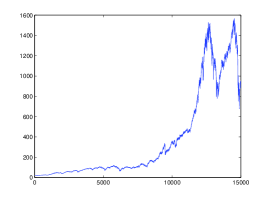
(a) S&P 500

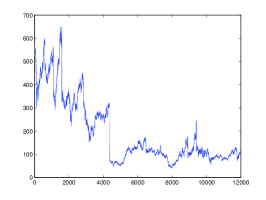
(b) IBM

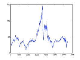
(c) JPM

Figure 1: Time values

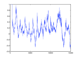
(a) S&P 500

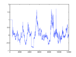
(b) IBM

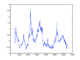
(c) JPM

Figure 2: Returns

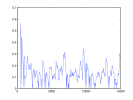
(a) S&P 500

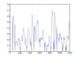
(b) IBM

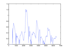
(c) JPM

Figure 3: Volatility of returns

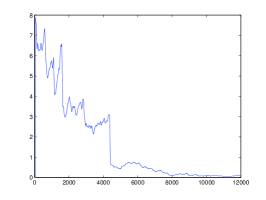
(a) Trend of IBM’s $\beta$

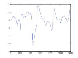
(b) Trend of R(IBM)’s $\beta$

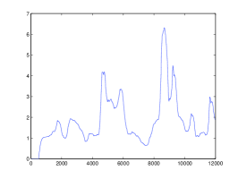
(c) Trend of $\beta$ of the volatility of R(IBM)

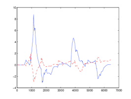
(d) Trends of R(IBM)’s $\beta_{1}$ (blue) and R(JPM)’s $\beta_{2}$ (red)

Figure 4: Betas

References

- (1) Adrian, T., Franzoni, F.: Learning about beta: Time-varying factor loadings, expected returns, and the conditional CAPM. J. Empirical Finance, vol. 16, pp. 537-556, 2009.
- (2) Béchu, T., Bertrand, E., Nebenzahl, J.: L’analyse technique ( éd.). Economica, 2008.
- (3) Bernstein, P.L.: Capital Ideas Evolving. Wiley, 2007.
- (4) Bodie, Z., Kane, A., Marcus, A.J.: Investments (7th ed.). McGraw-Hill, 2008.
- (5) Cartier, P., Perrin, Y.: Integration over finite sets. In F. & M. Diener (Eds): Nonstandard Analysis in Practice, pp. 195-204. Springer, 1995.
- (6) Diener, F., Diener, M.: Tutorial. In F. & M. Diener (Eds): Nonstandard Analysis in Practice, pp. 1-21. Springer, 1995.
- (7) Diener, F., Reeb, G.: Analyse non standard. Hermann, 1989.
- (8) Fliess, M.: Analyse non standard du bruit. C.R. Acad. Sci. Paris Ser. I, vol. 342, pp. 797-802, 2006.
-
(9)
Fliess, M.:
Critique du rapport signal à bruit en communications numériques. ARIMA,
vol. 9, pp. 419-429, 2008 (available at
http//hal.archives-ouvertes.fr/inria-00311719/en/). -
(10)
Fliess, M., Join, C.:
A mathematical proof of the existence of trends
in financial time series. In A. El Jai, L. Afifi, E. Zerrik (Eds):
Systems Theory: Modeling, Analysis and Control, , pp.
43-62. Presses Universitaires de Perpignan, 2009 (available at
http//hal.archives-ouvertes.fr/inria-00352834/en/). -
(11)
Fliess, M., Join, C.:
Systematic risk analysis:
first steps towards a new definition of beta. COGIS, Paris,
2009 (available at
http//hal.archives-ouvertes.fr/inria-00425077/en/). -
(12)
Fliess, M., Join, C.:
Preliminary remarks on option pricing and dynamic hedging. 1st Internat. Conf. Syst. Comput. Sci. , Villeneuve-d’Ascq, 2012 (available at
http//hal.archives-ouvertes.fr/hal-00705373/en). -
(13)
Fliess, M., Join, C.
Model-free control.
Internat. J. Control, vol. 86, pp. 2228-2252, 2013 (available at
http://hal.archives-ouvertes.fr/hal-00828135/en/). -
(14)
Fliess, M., Join, C., Hatt, F.:
Volatility made observable at last. 3es J. Identif. Modélisation Expérimentale,
Douai, 2011 (available at
http//hal.archives-ouvertes.fr/hal-00562488/en/). - (15) Fliess, M., Join, C., Hatt, F.: A-t-on vraiment besoin de modèles probabilistes en ingénierie financière? Conf. médit. ingénierie sûre systèmes complexes, Agadir, 2011 (available at http//hal.archives-ouvertes.fr/hal-00585152/en/).
- (16) Fliess, M., Join, C., Mboup, M.: Algebraic change-point detection. Applicable Algebra Engin. Communic. Comput., vol. 21, pp. 131-143, 2010.
- (17) Fliess, M., Join, C., Sira-Ramírez, H.: Residual generation for linear fault diagnosis: an algebraic setting with examples. Internat. J. Control, vol. 77, pp. 1223-1242, 2004.
-
(18)
Fliess, M., Join, C., Sira-Ramírez, H.:
Non-linear estimation is easy. Int. J. Model. Identif.
Control, vol. 4, pp. 12-27, 2008 (available at
http://hal.archives-ouvertes.fr/inria-00158855/en/). -
(19)
Fliess, M., Mboup, M., Mounier, H., Sira-Ramírez, H.:
Questioning some paradigms of signal processing via concrete examples. In H.
Sira-Ramírez, G. Silva-Navarro (Eds.): Algebraic Methods in
Flatness, Signal Processing and State Estimation, pp. 1-21,
Editiorial Lagares, 2003 (available at
http://hal.archives-ouvertes.fr/inria-00001059/en/). - (20) Fliess, M., Sira-Ramírez, H.: An algebraic framework for linear identification. ESAIM Control Optimiz. Calc. Variat., vol. 9, pp. 151–168, 2003.
- (21) Fliess, M., Sira-Ramírez, H.: Closed-loop parametric identification for continuous-time linear systems via new algebraic techniques. In H. Garnier, L. Wang (Eds): Identification of Continuous-time Models from Sampled Data, pp. 362-391. Springer, 2008.
- (22) Folland, G.B.: Advanced Calculus, Prentice Hall, 2002.
- (23) Gençay, R., Selçuk, F., Whitcher, B.: An Introduction to Wavelets and Other Filtering Methods in Finance and Economics. Academic Press, 2002.
- (24) Ince, E.L.: Ordinary Differential Equations. Longmans-Green, 1926.
- (25) Kirkpatrick, C.D., Dahlquist, J.R.: Technical Analysis: The Complete Resource for Financial Market Technicians (2nd ed.). FT Press, 2010.
- (26) Lobry, C., Sari, T.: Nonstandard analysis and representation of reality. Internat. J. Control, vol. 81, pp. 517-534, 2008.
- (27) Mboup, M.: Parameter estimation for signals described by differential equations. Applicable Analysis, vol. 88, pp. 29-52, 2009.
- (28) Mboup, M., Join, C., Fliess, M.: Numerical differentiation with annihilators in noisy environment. Numer. Algor., vol. 50, pp. 439-467, 2009.
- (29) Ross, S.: The arbitrage theory of capital asset pricing. J. Economic Theory, vol. 13, pp. 341-360, 1976.
- (30) Sharpe, W.F.: Capital asset prices: A theory of market equilibrium under conditions of risk. J. Finance, vol. 19, pp. 425-442, 1964.
- (31) Teräsvirta, T.: Forecasting economic variables with nonlinear models. In G. Elliott, C.W.J. Granger, A. Timmermann (Eds): Handbook of Economic Forecasting, vol. 1, pp. 413-457. North-Holland, 2006.
- (32) Tofallis, C.: Investment volatility: A critique of standard beta estimation and a simple way forward. Europ. J. Operat. Res., vol. 187, pp. 1358-1367, 2008.
- (33) Trapero, J.R., Sira-Ramírez, H., Feliu Battle, V.: An algebraic frequency estimator for a biased and noisy sinusoidal signal. Signal Processing, vol. 87, pp. 1188-1201, 2007.
- (34) Trapero, J.R., Sira-Ramírez, H., Feliu Battle, V.: A fast on-line frequency estimator of lightly damped vibrations in flexible structures. J. Sound Vibration, vol. 307 pp. 365-378, 2007.
- (35) Trapero, J.R., Sira-Ramírez, H., Feliu Battle, V.: On the algebraic identification of the frequencies, amplitudes and phases of two sinusoidal signals from their noisy sums. Internat. J. Control, vol. 81, pp. 505-516, 2008.
-
(36)
Ushirobira, R., Perruquetti, W., Mboup, M., Fliess, M.:
Algebraic parameter estimation of a biased sinusoidal waveform
signal from noisy data. 16th IFAC Symp. System
Identif., Brussels, 2012 (available at
http//hal.archives-ouvertes.fr/hal-00685067/en/).