Local structure approximation as a predictor of second order phase transitions in asynchronous cellular automata

1 Introduction

If the field of deterministic cellular automata is now relatively well known, their stochastic counterparts remains in great part terra incognita. Indeed, even in the simplest case where the systems are binary, one-dimensional, and where the behaviour of each cell of the automaton depends only on itself and its two nearest neighbours, little is known on the behaviour of such systems with random local transitions functions.

As a first step, we focus on this particular set of cellular automata, called Elementary Cellular Automata (ECA). We consider here $\alpha$-asynchronous rules, which are obtained by a random perturbation of the deterministic updating rule: instead of updating all cells simulatneously, we update each cell independently with probability $\alpha$, the synchrony rate, and leave its state unchanged with probability $1-\alpha$. Two main motivations exist for studying such systems:

• In the case where the cellular automaton is used to represent the evolution of a natural phenomenon, it is interesting to know what is the respective role of the local rule and the updating procedure in the outcome of a simulation [4, 16]. The study of a continuous variation of $\alpha$ for a quasi-deterministic setting ($\alpha\rightarrow 1$) to a quasi-sequential one ($\alpha\rightarrow 0$) may allow us to detect the non-robustness of some systems (see e.g. the study of Grilo and Correia on the iterated prisoner’s dilemma [12]).

• $\alpha$-asynchronous cellular automata can also be seen as the result of a stochastic “mixing” of two deterministic rules (the original rule and the identity rule). However, in contrast to other perturbations where the outcome of the mix can be partially predicted (e.g., mixing a rule with uniform noise or with a “null” rule), the effect of switching from the deterministic setting ($\alpha=1$) to a probabilistic one ($\alpha<1$) is to date unknown, even if $\alpha$ is infinitely close to $1$. The origin of this fact can be intuitively perceived by considering that, from the point of view of each single cell, all happens as if it were updated with an independent clock where the time between two updates follows a geometric law of parameter $\alpha$. It is therefore difficult, if not impossible, to predict in all generality whether the introduction of asynchrony will stabilize or destabilize the system [2, 8].

The systematic exploration of the properties of $\alpha$-asynchronous Elementary Cellular Automata by numerical simulations revealed that different “responses” to this perturbation were observed: some rules, as the majority rule (ECA 232), show only little change while other rules (e.g., ECA 2) show a drastic modification of their behaviour as soon as a little amount of asynchronism is introduced [7]. However, the most surprising phenomenon was the identification of rules which exhibited a qualitative change of behaviour for a continuous variation of the synchrony rate: there exists a critical value of $\alpha_{c}$ which separates a an active phase in which the system fluctuates around en equilibrium and an absorbing phase where the system is rapidly attracted towards a fixed point where all cells are in the same state.

Using the techniques from statistical physics, this abrupt change of behaviour was then identified as a second order phase transitions which belong to the directed percolation (DP) universality class [6]. This identification was conducted by taking as an order parameter the density, that is the average number of cells in state 1, and, up to symmetries, nine rules were found to exhibit such DP behaviour. Their Wolfram numbers is: 6, 18, 26, 38, 50, 58, 106, 134, and 146.

The aim of this paper is to study to which extent this second order phase transition can be predicted with analytical techniques. We are in particular interested in answering two questions: (a) Can we explain the existence of the two active and absorbing phases? (b) Can we propose an approximation of the value of the critical synchrony rate $\alpha_{c}$ that separates the two phases?

Our approach is based on so-called local structure theory, proposed in 1987 by H. A. Gutowitz et al. [14, 13] as a generalization of the mean-field theory for cellular automata. Unlike mean-field theory, local structure theory takes (partially) into account correlations between sites. The basic idea of this theory is to consider probabilities of blocks (words) of length $k$ and to construct a map on these block probabilities, which, when iterated, approximates probabilities of occurrence of the same blocks in the actual orbit of a given cellular automaton. The construction is based on the idea of “Bayesian extension”, introduced earlier by other authors in the context of lattice gases [3, 5], and also known as a “finite-block measure” or as “Markov process with memory”. Although Gutowitz et al. originally considered deterministic CA rules, extension to probabilistic rules is straightforward, and has been described in detail in [10]. In the case of nearest-neighbour binary rule, the aforementioned map is $2^{k}$-dimensional, where $k$ is called the level of local structure approximation. However, using the method proposed in [10], it can be reduced to equivalent, but somewhat simpler $2^{k-1}$ dimensional map, and we will fully exploit this simplification here.

It has been observed that for many CA rules, as the level $k$ increases, the accuracy of the approximation increases as well. More importantly, in some PCA, their local structure map “inherits” important features of the PCA. For example, Mendonça and de Oliveira [15] studied a PCA which can be understood as a “probabilistic mixture” of elementary CA rules 182 and 200, such that at a given site, rule 182 is applied with a probability $p$, and rule 202 with probability $1-p$. They found that as $p$ varies, the density of ones in the steady state undergoes a phase transition which, according to numerical evidence, belongs to DP (directed percolation) universality class. They also found that the mean-field approximation of this rule predicts existence of this phase transition, meaning that the mean field map exhibits a bifurcation with exchange of stability between two fixed points. For higher level local structure approximation (level 2, 3 and 4), the authors obtained density curves approximating the actual density curve with increasing accuracy as the level increased.

In the rest of this paper, we will demonstrate that for $\alpha$-asynchronous Elementary Cellular Automata exhibiting phase transitions belonging to DP universality class this is also the case: the local structure approximation not only predicts existence of the phase transition, but does that increasingly well as the level of the approximation increases.

2 Probabilistic cellular automata

We will assume that the dynamics takes place on a one-dimensional lattice. Let $s_{i}(t)$ denotes the state of the lattice site $i$ at time $t$, where $i\in\mathbb{Z}$, $t\in\mathbb{N}$. We will further assume that $s_{i}(t)\in\{0,1\}$ and we will say that the site $i$ is occupied (empty) at time $t$ if $s_{i}(t)=1$ ($s_{i}(t)=0$). Deterministic elementary cellular automaton is the dynamical system governed by the local function $f:\{0,1\}^{3}\to\{0,1\}$ such that

$$s_{i}(t+1)=f\big{(}s_{i-1}(t),s_{i}(t),s_{i+1}(t)\big{)}.$$

Function $f$ is be called a rule of CA.

In a probabilistic cellular automaton (PCA), lattice sites simultaneously change states form $0$ to $1$ or from $1$ to $0$ with probabilities depending on states of local neighbours. A common method for defining PCA is to specify a set of local transition probabilities. For example, in order to define a nearest-neighbour PCA one has to specify the probability $w(s_{i}(t+1))|s_{i-1}(t),s_{i}(t),s_{i+1}(t))$ that the site $s_{i}(t)$ with nearest neighbors $s_{i-1}(t),s_{i+1}(t)$ changes its state to $s_{i}(t+1)$ in a single time step.

A more formal definition of nearest-neighbour PCA can be constructed as follows. Consider a set of independent Boolean random variables $X_{i,\mathbf{b}}$, where $i\in\mathbb{Z}$ and $\mathbf{b}\in\{0,1\}^{3}$. Probability that the random variable $X_{i,\mathbf{b}}$ takes the value $a\in\{0,1\}$ will be assumed to be independent of $i$ and denoted by $w(a|\mathbf{b})$,

$$Pr(X_{i,\mathbf{b}}=a)=w(a|\mathbf{b}).$$ (1)

Obviously, $w(1|\mathbf{b})+w(0|\mathbf{b})=1$ for all $\mathbf{b}\in\{0,1\}^{n}$. The update rule for PCA is then defined by

$$s_{i}(t+1)=X_{i,\{s_{i+l}(t),s_{i+l+1}(t),\ldots,s_{i+r}(t)\}}.$$ (2)

Note that new random variables $X$ are used at each time step $t$, that is, random variables $X$ used at time step $t$ are independent of those used at previous time steps.

With the above definition, it is clear that in order to fully define a nearest-neighbour PCA rule, it is enough to specify eight transition probabilities $w(1|x_{1}x_{2}x_{3})$ for all $x_{1},x_{2},x_{3}\in\{0,1\}$. Remaining eight probabilities, $w(0|x_{1}x_{2}x_{3})$, can be obtained by $w(0|x_{1}x_{2}x_{3})=1-w(1|x_{1}x_{2}x_{3})$.

We will now define $\alpha$-asynchronous elementary cellular automata. Let $\alpha\in[0,1]$ and let $f$ be a local function of some deterministic CA with Wolfram number $W(f)$. Corresponding $\alpha$-asynchronous elementary cellular automaton with rule number $W(f)$ is a probabilistic CA for which transition probabilities are

$$w(1|x_{1}x_{2}x_{3})=\alpha f(x_{1},x_{2},x_{3})+(1-\alpha)x_{2}.$$ (3)

Note that when $\alpha=1$, the above becomes just the deterministic rule with local function $f$, and when $\alpha=0$, it becomes the identity rule.

3 Local structure approximation

In what follows we assume that the probabilistic CA rule is binary and that the neighbourhood size is three (central site and two nearest neighbours). It is not difficult, however, to generalize these results to CA with higher number of states and larger neighbourhood.

We denote by $P_{t}(\mathbf{b})$ the probability of occurrences of blocks $\mathbf{b}=b_{1}b_{2}\ldots b_{n}$ after $t$ iterations of the PCA rule, where $\mathbf{b}\in\{0,1\}^{*}$, that is, $\mathbf{b}$ is a word over the binary alphabet. More precisely,

$$P_{t}(\mathbf{b})=Pr\Big{(}s_{i}(t)=b_{1},s_{i+1}(t)=b_{2},\ldots s_{i+n-1}(t)=b_{n}\Big{)},$$ (4)

where we assume that $P_{t}(\mathbf{b})$ is independent of $i$, since we will be only interested in shift-invariant states.

One should add at this point that the block probabilities $P_{t}(\mathbf{b})$, as we will call them, are more formally measures of cyllinder sets with respect to a shift-invariant measure on $\{0,1\}^{\mathbb{Z}}$. Review of all details of the construction of this measure can be found in [10], thus we will not discuss these details here. We will only remark that the knowledge of all block probabilities is equivalent to the knowledge of probability measure on $\{0,1\}^{\mathbb{Z}}$, by the virtue of Hahn-Kolmogorov extension theorem [10]. Therefore, the sequence of sets of block probabilities

$$\{P_{t}(\mathbf{b}):\,\,\mathbf{b}\in\{0,1\}^{\star}\}$$

with $t=0,1,2\ldots$ can be viewed as a sequence of probability measures on $\{0,1\}^{\mathbb{Z}}$. Moreover, if $P_{t}(\mathbf{b})=P_{t+1}(\mathbf{b})$ for all $\mathbf{b}$, then these block probabilities define invariant measure. It has been observed that in many PCA rules, as $t\to\infty$, block probabilities tend to some stationary or “equilibrium” value. These stationary block probability values will be denoted by $P(\mathbf{b})$, that is, without index $t$. Obviously, they extend to invariant measures.

In some cases, for blocks $\mathbf{b}$ of short lenght, one can calculate $P_{t}(\mathbf{b})$ directly, as, for example, has been done for $\alpha$-asynchronous ECA rules 76, 140 and 200 in [11]. For $\alpha$-asynchronous rules exhibiting phase transitions such direct calculations are not possible, thus we will use approximate method known as local structure theory.

Block probabilities form an infinite hierarchy

$P_{t}(0),P_{t}(1)$

$P_{t}(00),P_{t}(01),P_{t}(10),P_{t}(11)$

$P_{t}(000),P_{t}(001),P_{t}(010),P_{t}(011),P_{t}(100),P_{t}(101),P_{t}(110),P_{t}(111)$

$\cdots$

that we can arrange by defining $\mathbf{P}_{t}^{(k)}$ as a column vector that holds all the $k$-block probabilities sorted in lexical order, that is,

$$\mathbf{P}_{t}^{(1)} =[P_{t}(0),P_{t}(1)]^{T},$$

$$\mathbf{P}_{t}^{(2)} =[P_{t}(00),P_{t}(01),P_{t}(10),P_{t}(11)]^{T},$$

$$\mathbf{P}_{t}^{(3)} =[P_{t}(000),P_{t}(001),P_{t}(010),P_{t}(011),P_{t}(100),P_{t}(101),P_{t}(110),P_{t}(111)]^{T},$$

$$\cdots.$$

Components of $\mathbf{P}_{t}^{(k)}$ are not independent: they obey relationships known as consistency conditions, which have the form

$$P_{t}(\mathbf{b})=P_{t}(\mathbf{b}0)+P_{t}(\mathbf{b}1)=P_{t}(0\mathbf{b})+P_{t}(1\mathbf{b})$$ (5)

for any block $\mathbf{b}$. These consistency conditions imply that generally only half of components of $\mathbf{P}_{t}^{(k)}$ are independent [10].

Let us now suppose that a PCA is given, and we know its transition probabilities $w$. Let $\mathbf{a}=a_{1}a_{2}\ldots a_{k}$ and $\mathbf{b}=b_{1}b_{2}\ldots b_{k+2}$ be two words of size $k$ and $k+2$, respectively, then the probability that blocks $\mathbf{a}$ results from an application of the local rule to block $\mathbf{b}$ is given by

$$w(\mathbf{a}|\mathbf{b})=\prod_{i=1}^{k}w(a_{i}|b_{i}b_{i+1}b_{i+2}),$$ (6)

where we took advantage of the fact that cells are independent. We can thus write:

$$P_{t}(\mathbf{a})=\sum_{\mathbf{b}\in\{0,1\}^{k+2}}w(\mathbf{a}|\mathbf{b})P_{t}(\mathbf{b}),$$ (7)

or, equivalently in matrix notation

$${\mathbf{P}_{t+1}^{(k)}}=W^{(k)}{\mathbf{P}_{t}^{(k+2)}},$$

where $W^{(k)}$ is a binary matrix with $2^{k}$ rows and $2^{k+2}$ columns with entries given by eq. (6).

If an invariant measure exists, then it is given by the set of block probability vectors ${\mathbf{P}^{(k)}}$, $k\in\mathbb{N}$, satisfying

$${\mathbf{P}^{(k)}}=W^{(k)}{\mathbf{P}^{(k+2)}}.$$

Thus, if we want to know what are the block probabilities for blocks of length $k$, we need to solve the above equation. The problem is that to know ${\mathbf{P}^{(k)}}$, one needs to know ${\mathbf{P}^{(k+2)}}$.

One possible solution is to approximate $\mathbf{P}^{(k+2)}$ by expressing it in terms of $\mathbf{P}^{(k)}$. Such approximation is known as Bayesian extension [14], and is given by

$$P(b_{1}b_{2}\ldots b_{k+2})\approx\begin{cases}P(b_{1})P(b_{2})P(b_{3})&\text{if $k=1$},\\[3.99994pt] \displaystyle\frac{P(b_{1}\ldots b_{k})P(b_{2}\ldots b_{k+1})P(b_{3}\ldots b_{k+2})}{P(b_{2}\ldots b_{k})P(b_{3}\ldots b_{k+1})}&\text{if $k>1$}.\end{cases}$$ (8)

where we assume that the denominator is positive. If the denominator is zero, then we take $P(b_{1}b_{2}\ldots b_{k+2})=0$. In order to avoid writing separate cases for denominator equal to zero, we define “thick bar” fraction as

$$\genfrac{}{}{1.0pt}{}{a}{b}:=\begin{cases}{\displaystyle\frac{a}{b}}&\mathrm{if\,\,}b\neq 0\\[10.00002pt] 0&\mathrm{if\,\,}b=0.\end{cases}$$ (9)

Moreover, in order to avoid writing the $k=1$ case separately, we adopt notational convention that

$$P(a_{m}\ldots a_{n})=1\mathrm{\,\,whenever\,\,}n<m,$$ (10)

and then we can write eq. (8) simply as

$$P(b_{1}b_{2}\ldots b_{k+2})\approx\genfrac{}{}{1.0pt}{}{P(b_{1}\ldots b_{k})P(b_{2}\ldots b_{k+1})P(b_{3}\ldots b_{k+2})}{P(b_{2}\ldots b_{k})P(b_{3}\ldots b_{k+1})},$$ (11)

which remains valid even for $k=1$.

The numerator of the fraction on the right hand side of eq. (11) contains only blocks of length $k$, and the denominator only blocks of length $k-1$. We can, however, express $k-1$ blocks by $k$ blocks using consistency conditions,

$$P(b_{2}\ldots b_{k}) =P(b_{2}\ldots b_{k}0)+P(b_{2}\ldots b_{k}1),$$ (12)

$$P(b_{3}\ldots b_{k+1}) =P(b_{3}\ldots b_{k+1}0)+P(b_{3}\ldots b_{k+1}1).$$ (13)

With the approximation given in eq. (11), for $k>1$, eq. (7) becomes

$$P_{t+1}(a_{1}\ldots a_{k})=\\ \sum_{b\in\{0,1\}^{k+2}}\prod_{i=1}^{k}w(a_{i}|b_{i}b_{i+1}b_{i+2})\genfrac{}{}{1.0pt}{}{P_{t}(b_{1}\ldots b_{k})P_{t}(b_{2}\ldots b_{k+1})P_{t}(b_{3}\ldots b_{k+2})}{\big{(}P_{t}(b_{2}\ldots b_{k}0)+P_{t}(b_{2}\ldots b_{k}1)\big{)}\big{(}P_{t}(b_{3}\ldots b_{k+1}0)+P_{t}(b_{3}\ldots b_{k+1}1)\big{)}},$$ (14)

and it should be understood as a system of $2^{k}$ equations, so that we have a separate equation for each $(a_{1}\ldots a_{k})\in\{0,1\}^{k}$. In vector form we will write

$$\mathbf{P}^{(k)}_{t+1}=\varLambda^{(k)}\left(\mathbf{P}^{(k)}_{t}\right),$$ (15)

where $\varLambda^{(k)}$, defined by eq. (14), will be called local structure map of level $k$. As we will see, for $\alpha$-asynchronous cellular automata, behaviour of fixed points of the local structure maps as a function of the synchrony rate $\alpha$ can be used as a predictor of existence of phase transitions.

We already mentioned that due to consistency conditions, not all components of the block probability vector $\mathbf{P}_{t}^{(k)}$ are independent. For example, for $k=3$, it is sufficient to consider only first four components of $\mathbf{P}_{t}^{(3)}$, that is, $P_{t}(000),P_{t}(001),P_{t}(010),P_{t}(011)$. The remaining four can be expressed as

$$P_{t}(100) =P_{t}(001),$$

$$P_{t}(101) =-P_{t}(001)+P_{t}(010)+P_{t}(011),$$

$$P_{t}(110) =P_{t}(011),$$

$$P_{t}(111) =1-P_{t}(000)-P_{t}(001)-2P_{t}(010)-3P_{t}(011).$$

These substitutions can be used to reduce $\varLambda^{(3)}$, the eight-dimensional local structure map of level 3, to a four-dimensional map. The same can be done for arbitrary $k$. Although $\varLambda^{(3)}$ has $2^{k}$ components, not all of them are independent, and with the help of consistency conditions it can be reduced to $2^{k-1}$ components [10].

For $k=1$, eq. (7) takes a simpler form,

$$P_{t+1}(a)=\sum_{\mathbf{b}\in\{0,1\}^{3}}w(a|b_{1}b_{2}b_{3})P(b_{1})P(b_{2})P(b_{3}),$$ (16)

where $a\in\{0,1\}$. This defines the two-dimensional map $\varLambda^{(1)}$,

$$\mathbf{P}^{(1)}_{t+1}=\varLambda^{(1)}\left(\mathbf{P}^{(1)}_{t}\right),$$ (17)

which we will call the mean-field map. Although this is an $\mathbb{R}^{2}\rightarrow\mathbb{R}^{2}$ map, again consistency conditions reduce it to one-dimensional map. Mean-filed map can be considered a special case of local structure map corresponding to $k=1$ (that is, the first-level of local structure approximation).

For $\alpha$-asynchronous rules,

$$w(1|b_{1}b_{2}b_{3}) =\alpha f(b_{1},b_{2},b_{3})+(1-\alpha)b_{2},$$ (18)

$$w(0|b_{1}b_{2}b_{3}) =1-w(1|b_{1}b_{2}b_{3}),$$ (19)

where $b_{1},b_{2},b_{3}\in\{0,1\}$. Equation (16) for $a=1$ thus takes the form

$$P_{t+1}(1)=\sum_{b_{1},b_{2},b_{3}\in\{0,1\}^{3}}\big{(}\alpha f(b_{1},b_{2},b_{3})+(1-\alpha)b_{2}\big{)}P_{t}(b_{1})P_{t}(b_{2})P_{t}(b_{3}).$$ (20)

Note that the second term will be non-zero only when $b_{2}=1$, and that summations of the second term over $b_{1}$ and $b_{3}$ yield factor $1$ due to consistency conditions $P_{t}(0)+P_{t}(1)=1$. We obtain, therefore,

$$P_{t+1}(1)=\alpha\sum_{b_{1},b_{2},b_{3}\in\{0,1\}^{3}}f(b_{1},b_{2},b_{3})P_{t}(b_{1})P_{t}(b_{2})P_{t}(b_{3})+(1-\alpha)P_{t}(1).$$ (21)

In the above, the sum $\sum f(b_{1},b_{2},b_{3})P_{t}(b_{1})P_{t}(b_{2})P_{t}(b_{3})$ will be a function of $P_{t}(1)$ and $P_{t}(0)$, but by substitution $P_{t}(1)=1-P_{t}(0)$ we can convert it to a function of $P_{t}(1)$ only, to be denoted $G(P_{t}(1))$, yielding

$$P_{t+1}(1)=\alpha G(P_{t}(1))+(1-\alpha)P_{t}(1),$$ (22)

or equivalently

$$P_{t+1}(1)=P_{t}(1)+\alpha\big{(}G(P_{t}(1))-P_{t}(1)\big{)}.$$ (23)

The above mean-field map of $\alpha$-asynchronous rule has fixed points given by

$$G(P_{t}(1))-P_{t}(1)=0,$$ (24)

and it is clear that they do not depend on $\alpha$. This means, in particular, that the mean-field map of $\alpha$-asynchronous rule has the same fixed point(s) as the mean-field map of the corresponding synchronous rule (for which $\alpha=1$).

4 Transcritical bifurcation

Before we continue, a brief interjection regarding transcritical bifurcations would be in place. As an example, let us consider the well-known logistic map

$$x\rightarrow\lambda x(1-x),$$ (25)

where $x\in[0,1]$. The parameter $\lambda$ is normally assumed to be in the interval $[0,4]$, but we will be interested in only a smaller interval, say $\lambda\in[1/2,2]$. The logistic map has two fixed points, $x^{-}=0$ and $x^{+}=(\lambda-1)/\lambda$. It is easy to show that for $\lambda<1$, $x^{-}$ is stable and $x^{+}$ is unstable, whereas for $\lambda>1$ their roles reverse, that is, $x=0$ is unstable and $x=(\lambda-1)/\lambda$ is stable. At $\lambda=1$ we thus observe an exchange of stability between fixed points, and such phenomenon is known as a transcritical bifurcation. Figure 1 shows the bifurcation diagram of the logistic map in the interval $[1/2,2]$, that is, graphs of both fixed points as a function of $\lambda$.

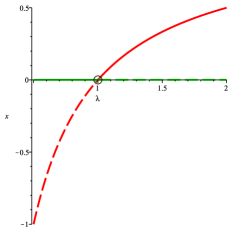
Figure 1: Bifurcation diagram for the logistic map. Solid line represents stable fixed point, dashed line unstable fixed point. Transcritical bifurcation point at $\lambda=1$ is circled.

Exchange of stability between two fixed points can also happen in higher-dimensional maps, including local structure maps, as we will shortly see below.

5 Local structure approximation for $\alpha$-ECA 6

The first example we are going to consider is $\alpha$-asynchronous elementary cellular automaton with rule code 6, defined by

$$w(1|000) =0,\,\,\,w(1|001)=\alpha,\,\,\,w(1|010)=1,\,\,\,w(1|011)=1-\alpha,$$ (26)

$$w(1|100) =0,\,\,\,w(1|101)=0,\,\,\,w(1|110)=1-\alpha,\,\,\,w(1|111)=1-\alpha.$$ (27)

For $k=1$, that is, for the mean-field approximation, we obtain, from eq. (16),

$$P_{t+1}(0) =P_{t}(0)^{3}+(2-\alpha)P_{t}(1)P_{t}(0)^{2}+(1+2\alpha)P_{t}(1)^{2}P_{t}(0)+\alpha P_{t}(1)^{3},$$ (28)

$$P_{t+1}(1) =(1+\alpha)P_{t}(1)P_{t}(0)^{2}+2(1-\alpha)P_{t}(1)^{2}P_{t}(0)+(1-\alpha)P_{t}(1)^{3}.$$ (29)

Consistency condition $P_{t}(0)+P_{t}(1)=1$ allows to eliminate one of the variables, thus we obtain the one-dimensional map

$$P_{t+1}(1)=(1+\alpha)P_{t}(1)-4\alpha P_{t}(1)^{2}+2\alpha P_{t}(1)^{3}.$$ (30)

Its fixed points are $0,1+\frac{\sqrt{2}}{2},1-\frac{\sqrt{2}}{2}$, and among them, only $0$ is in the interval $[0,1]$, thus it is the only admissible fixed point. Since this fixed point is independent of $\alpha$, the mean field obviously does not exhibit any bifurcation, and we have to consider higher order of the local structure approximation.

For $k=2$, we have $2^{2}=4$ local structure equations given by eq. (14). Assuming that denominators are not zero, and replacing the “thick bar” by a regular one, using variables $x_{t}=P_{t}(00)$, $y_{t}=P_{t}(10)$, $z_{t}=P_{t}(10)$, and $v_{t}=P_{t}(11)$, eqs. (14) after simplification become

$$x_{t+1}=\frac{1}{(z_{t}+v_{t})(x_{t}+y_{t})^{2}}\{v_{t}(x_{t}+y_{t})(v_{t}x_{t}+y_{t}v_{t}+y_{t}^{2}){\alpha}^{2}\\ +(-x_{t}y_{t}{z_{t}}^{2}+2y_{t}v_{t}z_{t}x_{t}-z_{t}x_{t}^{2}y_{t}+z_{t}x_{t}^{2}v_{t}+x_{t}y_{t}^{2}v_{t}+2y_{t}^{2}v_{t}z_{t})\alpha\\ +x_{t}(z_{t}+x_{t})(x_{t}+y_{t})(z_{t}+v_{t})\},$$ (31)

$$y_{t+1}=\frac{1}{(z_{t}+v_{t})(x_{t}+y_{t})^{2}}\{-v_{t}(x_{t}+y_{t})(v_{t}x_{t}+y_{t}v_{t}+y_{t}^{2}){\alpha}^{2}\\ +(x_{t}y_{t}{z_{t}}^{2}-y_{t}^{2}v_{t}z_{t}-z_{t}x_{t}y_{t}^{2}+2x_{t}y_{t}v_{t}^{2}+y_{t}^{3}v_{t}+v_{t}^{2}x_{t}^{2}+y_{t}^{2}v_{t}^{2})\alpha\\ +y_{t}(z_{t}+x_{t})(x_{t}+y_{t})(z_{t}+v_{t})\},$$ (32)

$$z_{t+1}=\frac{-v_{t}(v_{t}x_{t}+y_{t}v_{t}+y_{t}^{2}){\alpha}^{2}+v_{t}(x_{t}+y_{t})(-z_{t}+y_{t}+v_{t})\alpha+z_{t}(x_{t}+y_{t})(y_{t}+v_{t})}{(z_{t}+v_{t})(x_{t}+y_{t})},\mbox{\hskip 39.83368pt}$$ (33)

$$v_{t+1}=\frac{v_{t}(v_{t}x_{t}+y_{t}v_{t}+y_{t}^{2}){\alpha}^{2}+(x_{t}y_{t}z_{t}-2y_{t}^{2}v_{t}-2v_{t}^{2}x_{t}-2y_{t}v_{t}^{2}-x_{t}y_{t}v_{t})\alpha+v_{t}(x_{t}+y_{t})(y_{t}+v_{t})}{(z_{t}+v_{t})(x_{t}+y_{t})}.$$ (34)

Because of consistency conditions, only first two variables are independent, and the remaining ones can be expressed by the first two as

$$z_{t} =P_{t}(10)=P_{t}(01)=y_{t},$$ (35)

$$v_{t} =P_{t}(11)=1-P_{t}(00)-P_{t}(01)-P_{t}(10)=1-x_{t}-2y_{t}.$$ (36)

This allows to reduce the original system to only two equations, with variables $x$ and $y$. We can then find fixed point of this system by dropping indices $t$ and $t+1$, and solving it for $x$ and $y$. This can be done with the help of a symbolic algebra software, yielding

$$x=P(00) =\frac{\alpha+1-(1-\alpha)\sqrt{4\alpha+1}}{2\alpha(2-\alpha)},$$ (37)

$$y=P(01) =\frac{\alpha-1+(1-\alpha)\sqrt{4\alpha+1}}{2\alpha(2-\alpha)},$$ (38)

$$z=P(10) =\frac{\alpha-1+(1-\alpha)\sqrt{4\alpha+1}}{2\alpha(2-\alpha)},$$ (39)

$$v=P(11) =\frac{\alpha-2\alpha^{2}+1-(1-\alpha)\sqrt{4\alpha+1}}{2\alpha(2-\alpha)}.$$ (40)

It is easy to check that this further yields

$$P(1)=1-P(0)=1-(P(00+P(01))=1-x-y=\frac{1-\alpha}{2-\alpha},$$ (41)

which remains positive for $\alpha\in[0,1)$. One can, moreover, show that the above fixed point is always stable. Because of the “thick bar” convention, one also demonstrate that equations (14) have in the case of $k=2$ also another fixed point, $x=1$, $y=z=v=0$. One can show that it is always unstable. This means that the local structure map of level 2 does not undergo any bifurcation, and that the local structure theory of level 2 does not predict any abrupt change in the density of ones as $\alpha$ changes. We need, therefore, to consider level 3 approximation.

For $k=3$, we have 8 equations given by (14), but again, only four of them are independent because of consistency conditions. These four are still rather complicated, thus, to save some space occupied by indices, we will write $\varLambda^{(3)}$ map instead of equations (14), and we will relegate some longer expressions to the Appendix. Assuming that denominators in (14) are positive, taking into account consistency conditions, and using variables $x=P(000),y=P(001),z=P(010)$ and $v=P(011)$, these four components of $\varLambda^{(3)}$ become

$$x \rightarrow\frac{-d_{x}}{(x+y)(y+v)^{2}},$$ (42)

$$y \rightarrow\frac{d_{y}}{(x+y)(y+v)^{2}},$$ (43)

$$z \rightarrow\frac{d_{z}}{y+v},$$ (44)

$$v \rightarrow\frac{-d_{v}}{(x+y)(y+v)^{2}},$$ (45)

where $d_{x}$, $d_{y}$, $d_{z}$ and $d_{v}$ are rather complicated polynomials, defined in the Appendix. Replacing arrows by equalities, we obtain a system of equations for fixed point. In order to solve it, it is convenient to change variables to $X=1-x-2y-v,Y=y+v,Z=z,V=x$, or equivalently $x=V,y=-V-Y+1-X,z=Z,v=V+2Y+X-1$. This change of variables is purposefully constructed in order to simplify the map, and the rationale for this choice is explained in [10], where it is called “short block representation”. In terms of block probabilities, these new variables are

$$X =P(1),$$ (46)

$$Y =P(01),$$ (47)

$$Z =P(010),$$ (48)

$$V =P(000).$$ (49)

We then obtain

$$X \rightarrow X-\alpha(2X+Y-Z+V-1)$$ (50)

$$Y \rightarrow Y+\frac{Z}{Y}(X+V-1)\alpha^{2}+(1-2X+Z-V)\alpha^{2}+(X-2Y+Z)\alpha$$ (51)

$$Z \rightarrow Z+{\frac{Z}{Y}}(V+X-1)(\alpha^{3}+\alpha)-\left(2X-Y+V-1\right){\alpha}^{3}$$ (52)

$$\mbox{\hskip 142.26378pt}+\left(X-4Y+3Z\right){\alpha}^{2}+\left(2Y-Z\right)\alpha$$

$$V \rightarrow V+\frac{\alpha}{(X+Y-1)^{2}Y^{2}}d_{V},$$ (53)

where

$$d_{V}=(X+Y-1)(2XY-XZ-Y^{2}+YV-ZV-Y+Z)Y\alpha^{2}\\ (Y-Z)(3X^{2}Y-X^{2}Z+9XY^{2}-3XYZ+4XYV-XZV+6Y^{3}-2Y^{2}Z+4Y^{2}V\\ -YZV+YV^{2}-6XY+2XZ-9Y^{2}+3YZ-4YV+ZV+3Y-Z)\alpha\\ -(X+Y+V-1)(2XY-2XZ+2Y^{2}-2YZ+YV-2Y+2Z)Y.$$ (54)

Fixed point of the above map can be obtained with the help of Maple symbolic solver, yielding

$$X =\frac{(1-\alpha)}{d_{\alpha}}(\alpha^{6}-5\alpha^{5}+10\alpha^{4}-7\alpha^{3}-2\alpha^{2}+4\alpha+2)(\alpha^{6}-7\alpha^{5}+19\alpha^{4}-23\alpha^{3}+8\alpha^{2}+8\alpha-4),$$ (55)

$$Y =\frac{1-\alpha}{d_{\alpha}}\left({\alpha}^{3}-2{\alpha}^{2}+\alpha+2\right)\left({\alpha}^{6}-7{\alpha}^{5}+19{\alpha}^{4}-23{\alpha}^{3}+8{\alpha}^{2}+8\alpha-4\right),$$ (56)

$$Z =\frac{1-\alpha}{d_{\alpha}}\left({\alpha}^{2}-2\alpha+2\right)\left({\alpha}^{6}-7{\alpha}^{5}+19{\alpha}^{4}-23{\alpha}^{3}+8{\alpha}^{2}+8\alpha-4\right),$$ (57)

$$V =\frac{{\alpha}^{2}}{d_{\alpha}}\left({\alpha}^{3}-2{\alpha}^{2}+\alpha+2\right)\left({\alpha}^{2}-3\alpha+3\right)\left(2{\alpha}^{6}-14{\alpha}^{5}+40{\alpha}^{4}-55{\alpha}^{3}+28{\alpha}^{2}+13\alpha-16\right),$$ (58)

where

$$d_{\alpha}=2(\alpha^{12}-11\alpha^{11}+54\alpha^{10}-152\alpha^{9}+259\alpha^{8}-248\alpha^{7}+73\alpha^{6}+95\alpha^{5}-84\alpha^{4}-15\alpha^{3}+32\alpha^{2}+2\alpha-8).$$ (59)

We will call this fixed point “active”, since it corresponds to non-zero value of $X$. Graph of $X$, that is, $P(1)$, as a function of $\alpha$ for this fixed point is shown in Figure 3. It is clear that $P(1)$ becomes negative at some point $\alpha=\alpha_{c}$. The value $\alpha_{c}$ can be obtained by solving equation $X=0$, but unfortunately the solution is not expressible by elementary functions, thus we can only say that $\alpha_{c}$ must satisfy

$${\alpha_{c}}^{6}-7{\alpha_{c}}^{5}+19{\alpha_{c}}^{4}-23{\alpha_{c}}^{3}+8{\alpha_{c}}^{2}+8{\alpha_{c}}-4=0,$$ (60)

yielding numerical value of $\alpha_{c}=0.4827758301$. Since the $X$ component of the fixed point given by eq. (55) becomes negative for $\alpha>\alpha_{c}$, and we cannot have negative probability, one can expect that the fixed point becomes unstable for $\alpha>\alpha_{c}$. In order to verify this, we can use the following general property [1] of maps $\mathbb{R}^{n}\rightarrow\mathbb{R}^{n}$. In general, if $F:\mathbb{R}^{n}\rightarrow\mathbb{R}^{n}$ has a fixed point at $\mathbf{u}\in\mathbb{R}^{n}$, and the Jacobian of $F$ at $\mathbf{u}$ has only eigenvalues with magnitude less than one, than $\mathbf{u}$ is stable. If, on the other hand, magnitude of at least one of the eigenvalues of the Jacobian is greater than one, than $\mathbf{u}$ is unstable.

For the map $\mathbb{R}^{4}\rightarrow\mathbb{R}^{4}$ given by eqs. (50–53), all four eigenvalues of the Jacobian evaluated at the fixed point given by eq. (55) are real. Using symbolic algebra software, it is possible to obtain explicit expressions for these eigenvalues as a function of $\alpha$, but they are too complicated to be included here. Instead, we include their graphs, shown in Figure 2.

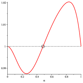
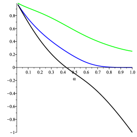
Figure 2: Graphs of eigenvalues of the Jacobian for rule 6. The eigenvalue which becomes larger than 1 for $\alpha>\alpha_{c}$ is shown on the left, while the remaining three eigenvalues on the right.

One can clearly see that magnitudes of three of these eigenvalues remain in the interval $[0,1]$, while the largest one becomes greater than one when $\alpha$ is sufficiently large. This happens when $\alpha>\alpha_{c}$, therefore we can conclude that the fixed point becomes unstable when $\alpha>\alpha_{c}$.

Remembering our “thick bar” convention, one can verify that there exists another fixed point of eqs. (14) for $k=3$. In terms of our new variables, it is given by $X=0,Y=0,Z=0,V=1$. We will call this fixed point “absorbing”. Its stability cannot be established by the same method, because the mapping given by eqs. (14) is not differentiable at this point. Nevertheless, it can be determined numerically by simply iterating the map and checking if it converges to the fixed point or not. Using this method, we verified that the fixed point $X=0,Y=0,Z=0,V=1$ is stable when $\alpha>\alpha_{c}$ and unstable for $\alpha<\alpha_{c}$. This means that at $\alpha=\alpha_{c}$ a transcritical bifurcation takes place, with exchange of stability between fixed points. This is illustrated in Figure 3, which shows bifurcation diagram for the $X$ component. We can therefore summarize our results by saying that the local structure approximation “predicts” that $P_{t}(1)$ behaves as follows

$$\lim_{t\to\infty}P_{t}(1)=\begin{cases}\frac{(1-\alpha)(\alpha^{6}-5\alpha^{5}+10\alpha^{4}-7\alpha^{3}-2\alpha^{2}+4\alpha+2)(\alpha^{6}-7\alpha^{5}+19\alpha^{4}-23\alpha^{3}+8\alpha^{2}+8\alpha-4)}{2(\alpha^{12}-11\alpha^{11}+54\alpha^{10}-152\alpha^{9}+259\alpha^{8}-248\alpha^{7}+73\alpha^{6}+95\alpha^{5}-84\alpha^{4}-15\alpha^{3}+32\alpha^{2}+2\alpha-8)}&\text{if $\alpha<\alpha_{c}$},\\ \mbox{\hskip 170.71652pt}0&\text{if $\alpha\geq\alpha_{c}$}.\end{cases}$$ (61)

Taylor expansion of the above expression for $\alpha<\alpha_{c}$ yields

$$\lim_{t\to\infty}P_{t}(1)=-A(\alpha-\alpha_{c})+O((\alpha-\alpha_{c})^{2})$$ (62)

where $A=30{\alpha_{c}}^{5}-272{\alpha_{c}}^{4}+917{\alpha_{c}}^{3}-1390{\alpha_{c}}^{2}+875{\alpha_{c}}-166$, which means that the local structure theory predicts, as expected, $\lim_{t\to\infty}P_{t}(1)\sim(\alpha-\alpha_{c})^{1}$, i.e., critical exponent $\beta=1$.

In conclusion, the local structure approximation at level three correctly predicts the existence of the phase transition in rule 6, and, moreover, it correctly predicts the direction of the transition: the active phase appears as $\alpha$ decreases. The critical value of $\alpha_{c}=0.4827758301$, however, is very far from the experimentally determined value reported in [9], which is $\alpha_{c}=0.2825$.

Rule 6                                                                       Rule 18

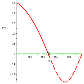
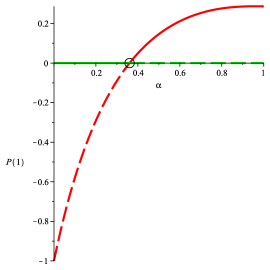
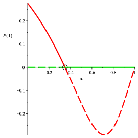
Rule 38

Figure 3: Bifurcation diagram for local structure equations of level three for rules 6, 18, and 38. Solid line represents stable fixed point, dashed line unstable fixed point. Transcritical bifurcation points are circled.

6 Local structure approximation for $\alpha$-asynchronous rules 18, 50, and 134

For rules 18, 50, and 134, the absorbing fixed point of the local structure map $\varLambda^{(3)}$ is the same as before, $X=0,Y=0,Z=0,V=1$. Active fixed point of $\varLambda^{(3)}$ can also be found using procedure outlined in the previous section, with the help of Maple symbolic algebra software. We only give expressions for the $X$ component of the fixed point, that is, for $P(1)$.

• Rule 18

  $$P(1)=\frac{-20{\alpha}^{5}+156{\alpha}^{4}-473{\alpha}^{3}+670{\alpha}^{2}-304{\alpha}+\sqrt[3]{A_{1}}-96}{24{\alpha}^{4}-120{\alpha}^{3}+270{\alpha}^{2}-96{\alpha}-192}\\ +\frac{A_{2}}{\sqrt[3]{A_{1}}(24{\alpha}^{4}-120{\alpha}^{3}+270{\alpha}^{2}-96{\alpha}-192)},$$ (63)

  where $A_{1}$ and $A_{2}$ are defined in the Appendix. The critical value $\alpha_{c}$ satisfies fourth order equation

  $$\alpha_{c}^{4}-7\alpha_{c}^{3}+16\alpha_{c}^{2}-16{\alpha_{c}}+4=0.$$ (64)

  Although it is possible to express $\alpha_{c}$ in terms of radicals, the expression is rather long, thus we only give its numerical value here, $\alpha_{c}=0.3605426781$.

• Rule 50

  $$P(1)=1-{\frac{(2{\alpha}^{2}-4\alpha+2)\sqrt{(1-\alpha)(16\alpha^{4}-57\alpha^{3}+95\alpha^{2}-75\alpha+25)}}{2(1-2{\alpha}^{2})(2{\alpha}^{2}-6\alpha+5)}}\\ +{\frac{8{\alpha}^{5}-34{\alpha}^{4}+58{\alpha}^{3}-56{\alpha}^{2}+35\alpha-10}{2(1-2{\alpha}^{2})(2{\alpha}^{2}-6\alpha+5)}}$$ (65)

  Bifurcation takes place at

  $$\alpha_{c}=\frac{5}{6}-\frac{1}{12}\,\left(188+12\,\sqrt{249}\right)^{1/3}+{\frac{2}{3}{\left({188+12\,\sqrt{249}}\right)^{-1/3}}}\approx 0.3233950179.$$ (66)

• Rule 134

  $$P(1)=1-2\,{\frac{115\,{\alpha}^{3}-298\,{\alpha}^{2}+280\,\alpha-90+3\left(5\alpha-4\right)\sqrt{8\,{\alpha}^{2}-16\,\alpha+9}}{575\,{\alpha}^{3}-1430\,{\alpha}^{2}+1253\,\alpha-378}}.$$ (67)

  The transcritical bifurcation occurs at $\alpha={\frac{31-\sqrt{41}}{46}}\approx 0.5347146906$.

In all three cases, we have exchange of stability of active and absorbing fixed point at $\alpha=\alpha_{c}$. Resulting bifurcation diagrams for rule 18 is shown in Figure 3, while diagrams for rule 50 and 134 in Figure 4.

Rule 50                                                                       Rule 106

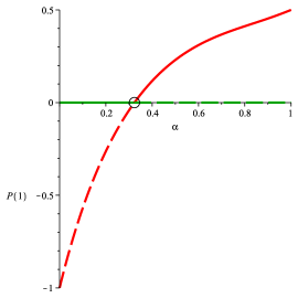
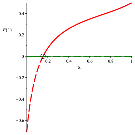
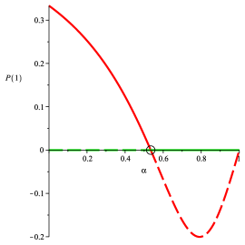
Rule 134

Figure 4: Bifurcation diagram for local structure equations of level three for rules 50, 106, and 134. Solid line represents stable fixed point, dashed line unstable fixed point. Transcritical bifurcation points are circled.

7 Remaining rules

For rule 38, the active fixed point of $\varLambda^{(3)}$ can be computed, but the expression is very long. The critical point $\alpha_{c}=0.3493360869$ is a solution of

$$8\alpha_{c}^{7}-42\alpha_{c}^{6}+106\alpha_{c}^{5}-155\alpha_{c}^{4}+142\alpha_{c}^{3}-82\alpha_{c}^{2}+28\alpha_{c}-4=0.$$ (68)

For rule 106, active fixed point of $\varLambda^{(3)}$ can also be computed, but, similarly as in the case of rule 38, the resulting formulas have hundreds of terms, thus we omit them here. The critical point $\alpha_{c}=0.1556040146$ is a solution of

$$18\alpha_{c}^{7}-131\alpha_{c}^{6}+464\alpha_{c}^{5}-1512\alpha_{c}^{4}+2678\alpha_{c}^{3}-2160\alpha_{c}^{2}+688\alpha_{c}-64=0.$$ (69)

Absorbing fixed points for rules 38 and 106 are the same as before, and $X=0,Y=0,Z=0,V=1$. Bifurcation diagrams of these rules are shown in Figures 3 and 4.

For the three remaining rules, 26, 58, and 146, the local structure map $\varLambda^{(3)}$ does not exhibit a transcritical bifurcation, so it is necessary to consider higher order maps, of level four (for rules 26 and 146) and five (for rule 58). Absorbing fixed points of these maps have the same structure as previously described, with $X=0$. Unfortunately, equations for their active fixed points cannot be solved even with the help of symbolic algebra software, due to the size of relevant equations. It is, however, possible to find the stable branch of the bifurcation diagram by iterating these maps many times, so they converge sufficiently close to the stable fixed point. We performed such iterations for all three cases, and the results are shown in Figure 5. Even though the unstable branch of the active fixed point is missing, it is evident that the active phase appears abruptly as $\alpha$ increases, which provides a strong evidence for transcritical bifurcation.

Rule 26                                                                       Rule 146

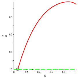
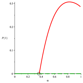
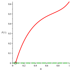
Rule 58

Figure 5: Partial bifurcation diagrams for local structure equations of level 4 rules 26 and 146, and level 5 for rule 58. Diagrams were obtained numerically with $10^{5}$ iterations. Solid line represents stable fixed point, dashed line unstable fixed point. Transcritical bifurcation points are circled.

8 Higher order local structure maps

As we could see in previous sections, local structure approximation of order 3 to 5 can predict existence of the phase transition for all DP rules. The local structure map for each of these rules exhibits a transcritical bifurcations, and the direction of the bifurcation agrees with the direction of the phase transition observed experimentally, that is, if the active phase appears (disappears) as $\alpha$ increases, then the non-zero fixed point of the local structure map becomes stable (unstable) as $\alpha$ increases. The point at which the transcritical bifurcation occurs is, however, rather far from the critical point observed experimentally. Thus one could say that the local structure approximation of order 3 to 5 approximates the value of $\alpha_{c}$ quite poorly.

Can this be improved by increasing the order of the local structure approximation? The answer is indeed yes, although we cannot expect to be able to find explicit symbolic expressions for fixed points of eq. (14) when $k$ is large. One can, however, iterate $\varLambda^{(k)}$ many times, starting from some generic initial condition, and when this is done, the orbit of $\varLambda^{(k)}$ indeed converges to a stable fixed point, which, depending on the value of $\alpha$, can be zero or non-zero.

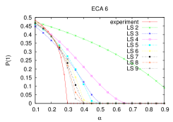
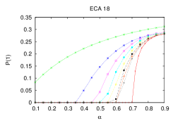
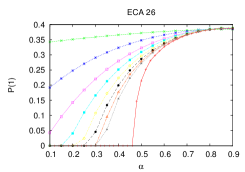
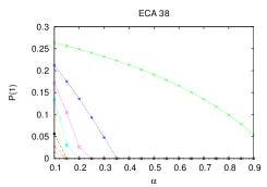
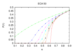
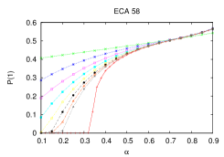
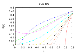
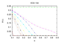
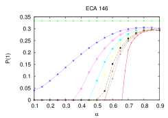
Figure 6: Experimental results together with local structure approximations up to level 9.

We performed iterations of $\varLambda^{(k)}$ maps for $k=2\ldots 9$ for all DP rules, and plotted $P_{t}(1)$ as a function of $\alpha$ after $t=10^{4}$ iterations. Results are shown in Figure 6, together with curves obtained “experimentally” by iterating a given rule for $10^{5}$ steps, using randomly generated initial configurations with $4\cdot 10^{4}$ sites and periodic boundary conditions. Once can clearly see that local structure maps not only predict existence of phase transitions, but also seem to approximate behaviour of density curves with increasing accuracy as the order of local structure approximation increases.

9 Conclusions

We have demonstrated that the local structure approximation of sufficiently high level correctly predicts existence of phase transitions in $\alpha$-asynchronous rules belonging to DP universality class. The phase transition manifests itself in local structure maps as transcritical bifurcation. The direction of the transition is predicted correctly by the local structure theory, and, more importantly, the location of the bifurcation point approximates better and better the location of the phase transition point as the level of local structure approximation increases.

Based on the evidence presented in this paper, we suspect that the same may be true for other probabilistic CA rules belonging to DP universality class. As mentioned in the introduction, it already known to be true for the probabilistic mixture of rules 182 and 200 studied by Mendonça and de Oliveira [15]. We plan to investigate this conjecture for other PCA rules.

At the same time, it seems that for rules which exhibit a phase transition, but do not belong to DP universality class, the local structure theory does not seem to predict existence of the phase transition at all. We investigated the only rule of this type among $\alpha$-asynchronous ECA, namely $\alpha$-asynchronous rule 178, belonging, according to [6], to $\mathrm{DP}_{2}$ universality class. We found that up to level 9, local structure maps for this rule do not exhibit any bifurcations.

The question why does the local structure predict existence of phase transitions in DP class, but fails for rules outside of this class, is obviously the most interesting one. While we were not able to answer this question so far, we might offer some plausible speculations. At the heart of the local structure approximation is the Bayesian extension, which can also be understood as maximal entropy approximation [10]. It is, therefore, reasonable to assume that for rules which produce somewhat “disordered” configurations, the local structure approximation may work well, whereas for rules exhibiting more “order” (or strongly pronounced spatio-temporal features), the approximation may be less accurate. Whether it is possible to express this conjecture in a more formal language, it remains to be seen.

10 Acknowledgments

H. Fukś acknowledges financial support from the Natural Sciences and Engineering Research Council of Canada (NSERC) in the form of Discovery Grant. This work was made possible by the facilities of the Shared Hierarchical Academic Research Computing Network (SHARCNET:www.sharcnet.ca) and Compute/Calcul Canada.

11 Appendix

Definitions of polynomials $d_{x}$, $d_{y}$, $d_{z}$ and $d_{v}$ for local structure equations for rule 6:

$$d_{x}=(x+y)(v+y)(3{v}^{2}+vx-zv-v+8yv+yx-y-2zy+5{y}^{2}){\alpha}^{3}\\ -(v+y-z)(3{v}^{2}x+3y{v}^{2}-vxz+3{y}^{2}v-zvy+4yvx+x{y}^{2}){\alpha}^{2}\\ -(v+y)y(2yv+vx+2{y}^{2}-2zy+yx-2xz)\alpha-x(v+y)^{2}(x+y)$$ (70)

$$d_{y}=(x+y)(v+y)(3{v}^{2}+vx-zv-v+8yv+yx-y-2zy+5{y}^{2}){\alpha}^{3}\\ +(6zvxy-17vx{y}^{2}-16{v}^{2}xy+2yvx+4{v}^{2}xz+4z{v}^{2}y+2zx{y}^{2}-2v{x}^{2}y+5{y}^{2}zv-{z}^{2}vx-yv{z}^{2}\\ -13{y}^{3}v-14{v}^{2}{y}^{2}-6x{y}^{3}-{v}^{2}{x}^{2}+{y}^{3}-{x}^{2}{y}^{2}-4{y}^{4}-5y{v}^{3}+y{v}^{2}+{v}^{2}x+{y}^{3}z+2{y}^{2}v+x{y}^{2}-5{v}^{3}x){\alpha}^{2}\\ +(v+y)(2y{v}^{2}+2{v}^{2}x+2yvx-2vxz-2zvy+{y}^{2}v-{y}^{3})\alpha+y(v+y)^{2}(x+y)$$ (71)

$$d_{z}=(3{v}^{2}+vx-zv-v+8yv+yx-y-2zy+5{y}^{2}){\alpha}^{3}\\ -(v+y)(5v-3z+x-1+6y){\alpha}^{2}+(2{y}^{2}+2{v}^{2}-3zy-2zv+4yv)\alpha+z(v+y)$$ (72)

$$d_{v}=(x+y)(v+y)(3{v}^{2}+vx-zv-v+8yv+yx-y-2zy+5{y}^{2}){\alpha}^{3}\\ +(7zvxy-29vx{y}^{2}-25{v}^{2}xy+4yvx+4{v}^{2}xz+4z{v}^{2}y+3zx{y}^{2}-4v{x}^{2}y\\ +6{y}^{2}zv-{z}^{2}vx-yv{z}^{2}-23{y}^{3}v-22{v}^{2}{y}^{2}-11x{y}^{3}-2{v}^{2}{x}^{2}+2{y}^{3}-2{x}^{2}{y}^{2}\\ -8{y}^{4}-7y{v}^{3}+2y{v}^{2}+2{v}^{2}x+2{y}^{3}z+4{y}^{2}v+2x{y}^{2}-7{v}^{3}x){\alpha}^{2}\\ +(v+y)(5y{v}^{2}+5{v}^{2}x+v{x}^{2}-3zvy+10yvx+8{y}^{2}v-vx-yv\\ -3vxz-{y}^{2}-{y}^{2}z+3{y}^{3}+5x{y}^{2}+{x}^{2}y-zxy-yx)\alpha-v(v+y)^{2}(x+y)$$ (73)

Definitions of $A_{1}$ and $A_{2}$ for eq. (63):

$$A_{1}=(2{\alpha}-3)(32{\alpha}^{14}+1776{\alpha}^{13}-32304{\alpha}^{12}\\ +248136{\alpha}^{11}-1156158{\alpha}^{10}+3746559{\alpha}^{9}-9102790{\alpha}^{8}+17374596{\alpha}^{7}-26738472{\alpha}^{6}\\ +33372704{\alpha}^{5}-33402048{\alpha}^{4}+26068992{\alpha}^{3}-14802944{\alpha}^{2}+5259264{\alpha}-884736)\\ +12\sqrt{3(8{\alpha}^{9}+56{\alpha}^{8}-426{\alpha}^{7}+940{\alpha}^{6}-821{\alpha}^{5}-588{\alpha}^{4}+2656{\alpha}^{3}-3220{\alpha}^{2}+1824{\alpha}-400)}\\ (4{\alpha}^{4}-20{\alpha}^{3}+45{\alpha}^{2}-16{\alpha}-32)(4{\alpha}^{6}-32{\alpha}^{5}+109{\alpha}^{4}-214{\alpha}^{3}+284{\alpha}^{2}-256{\alpha}+128)$$ (74)

$$A_{2}=16{\alpha}^{10}-576{\alpha}^{9}+5048{\alpha}^{8}-22816{\alpha}^{7}+65969{\alpha}^{6}-134476{\alpha}^{5}\\ +199844{\alpha}^{4}-213632{\alpha}^{3}+161536{\alpha}^{2}-82944{\alpha}+21504$$ (75)

References

- [1] K.T. Alligood, T. Sauer, and J.A. Yorke. Chaos: An Introduction to Dynamical Systems. Springer, 1997.
- [2] Hugues Bersini and Vincent Detours. Asynchrony induces stability in cellular automata based models. In Rodney A. Brooks and Pattie Maes, editors, Proceedings of the 4th International Workshop on the Synthesis and Simulation of Living Systems , pages 382–387. MIT Press, 1994.
- [3] H. J. Brascamp. Equilibrium states for a one dimensional lattice gas. Communications In Mathematical Physics, 21(1):56, 1971.
- [4] Buvel, R.L. and Ingerson, T.E. Structure in asynchronous cellular automata. Physica D, 1:59–68, 1984.
- [5] M. Fannes and A. Verbeure. On solvable models in classical lattice systems. Commun. Math. Phys., 96:115–124, 1984.
- [6] Nazim Fatès. Asynchronism induces second order phase transitions in elementary cellular automata. Journal of Cellular Automata, 4(1):21–38, 2009.
- [7] Nazim Fatès and Michel Morvan. An experimental study of robustness to asynchronism for elementary cellular automata. Complex Systems, 16:1–27, 2005.
- [8] Nazim Fatès, Michel Morvan, Nicolas Schabanel, and Eric Thierry. Fully asynchronous behavior of double-quiescent elementary cellular automata. Theoretical Computer Science, 362:1–16, 2006.
- [9] Nazim Fatès, A. Asynchronism Induces Second Order Phase Transitions in Elementary Cellular Automata. Journal of Cellular Automata, 4(1):21–38, 2008.
- [10] Henryk Fukś. Construction of local structure maps for cellular automata. J. of Cellular Automata, pages 1–30, 2012. In press.
- [11] Henryk Fukś and Andrew Skelton. Orbits of Bernoulli measure in asynchronous cellular automata. Dis. Math. Theor. Comp. Science, AP:95–112, 2011.
- [12] Carlos Grilo and Luís Correia. Effects of asynchronism on evolutionary games. Journal of Theoretical Biology, 269(1):109 – 122, 2011.
- [13] H. A. Gutowitz and J. D. Victor. Local structure theory in more than one dimension. Complex Systems, 1:57–68, 1987.
- [14] H. A. Gutowitz, J. D. Victor, and B. W. Knight. Local structure theory for cellular automata. Physica D, 28:18–48, 1987.
- [15] J. R. G. Mendonça and M. J. de Oliveira. An extinction-survival-type phase transition in the probabilistic cellular automaton p 182– q 200. J. of Phys. A: Math. and Theor., 44(15):art. no. 155001, 2011.
- [16] Birgitt Schönfisch and André de Roos. Synchronous and asynchronous updating in cellular automata. BioSystems, 51:123–143, 1999.