Abstract

On the basis of tidal despinning timescale arguments, Peale showed in 1977 that the majority of irregular satellites (with unknown rotation states) are expected to reside close to their initial (fast) rotation states. Here we investigate the problem of the current typical rotation states among all known satellites from a viewpoint of dynamical stability. We explore location of the known planetary satellites on the ($\omega_{0}$, $e$) stability diagram, where $\omega_{0}$ is an inertial parameter of a satellite and $e$ is its orbital eccentricity. We show that most of the satellites with unknown rotation states cannot rotate synchronously, because no stable synchronous 1:1 spin-orbit state exists for them. They rotate either much faster than synchronously (those tidally unevolved) or, what is much less probable, chaotically (tidally evolved objects or captured slow rotators).

1 Introduction

What is a typical rotation state of a planetary satellite? The majority of planetary satellites with known rotation states rotate synchronously (like the Moon, facing one side towards a planet), i.e., they move in synchronous spin-orbit resonance 1:1. The data of the NASA reference guide (http://solarsystem.nasa.gov/planets/, ) combined with additional data (on the rotation of Caliban (U16), Sycorax (U17) and Prospero (U18) (Maris et al., 2001, 2007) and the rotation of Nereid (N2) (Grav et al., 2003)) implies that, of the 33 satellites with known rotation periods, 25 rotate synchronously.

For the tidally evolved satellites, this observational fact is theoretically expected. Synchronous 1:1 resonance with the orbital motion is the most likely final mode of the long-term tidal evolution of the rotational motion of a planetary satellite (Goldreich and Peale, 1966; Peale, 1969, 1977).

Another qualitative kind of rotation known from observations is fast regular rotation. There are seven satellites known to rotate so (http://solarsystem.nasa.gov/planets/, ; Maris et al., 2001, 2007; Grav et al., 2003; Bauer et al., 2004): Himalia (J6), Elara (J7), Phoebe (S9), Caliban (U16), Sycorax (U17), Prospero (U18), and Nereid (N2); all of them are irregular satellites (with a possible exception of Nereid, see Sheppard, Jewitt, and Kleyna (2006) and references therein). The rotation periods of them are equal to $0.4$, $0.5$, $0.4$, $0.11$, $0.15$, $0.19$ and $0.48$ days, respectively; i.e., they are less than their orbital periods approximately 630, 520, 1400, 5200, 8600, 10300 and 750 times, respectively. These satellites, apparently, are tidally unevolved.

A third observationally discovered qualitative kind of rotation is chaotic tumbling. Wisdom et al. (1984) and Wisdom (1987) demonstrated theoretically that a planetary satellite of irregular shape in an elliptic orbit could rotate in a chaotic, unpredictable way. They found that a unique (at that time) probable candidate for the chaotic rotation, due to a pronounced shape asymmetry and significant orbital eccentricity, was Hyperion (S7). Besides, it has a small enough theoretical timescale of tidal deceleration of rotation from a primordial rotation state. Later on, a direct modelling of its observed light curves (Klavetter, 1989; Black et al., 1995; Devyatkin et al., 2002) confirmed the chaotic character of Hyperion’s rotation. Recent direct imaging from the CASSINI spacecraft supports these conclusions (Thomas et al., 2007).

It was found in a theoretical research (Kouprianov and Shevchenko, 2005) that two other Saturnian satellites, Prometheus (S16) and Pandora (S17), could also rotate chaotically (see also Melnikov and Shevchenko (2008)). Contrary to the case of Hyperion, possible chaos in rotation of these two satellites is due to occasional fine-tuning of the dynamical and physical parameters rather than to a large extent of a chaotic zone in the rotational phase space.

We see that the satellites spinning fast or tumbling chaotically are a definite minority among the satellites with known rotation states. However, the observed dominance of synchronous behaviour might be a selection effect, exaggerating the abundance of the mode typical for big satellites. This is most probable. Peale (1977) showed on the basis of tidal despinning timescale arguments that the majority of the irregular satellites are expected to reside close to their initial (fast) rotation states.

A lot of new satellites has been discovered during last years. Now the total number of satellites exceeds 160 (http://solarsystem.nasa.gov/planets/, ). The rotation states for the majority of them are not known. All small enough satellites have irregular shapes (and many of them large orbital eccentricities, see Sheppard (2006)), and this may result, as in the case of Hyperion (Wisdom et al., 1984), in the non-existence of attitude stable synchronous state; or, such a state may be even absent in the present epoch in the phase space of the planar rotational motion.

In this paper, we investigate the problem of the current typical rotation states among satellites from a viewpoint of dynamical stability, considering tidal timescale estimates as supplementary argumentation solely. We explore location of the known planetary satellites on the ($\omega_{0}$, $e$) stability diagram, where $\omega_{0}$ is an inertial parameter of a satellite and $e$ is its orbital eccentricity. Using an empirical relationship connecting the size of a satellite and its figure asymmetry, we locate almost all known satellites on this diagram. Then, by means of analysis of the residence of satellites in various domains of stability/instability in this diagram, we draw conclusions on the rotation states that are expected to be predominant among the planetary satellites. Note that our argumentation is independent from the postulates of the tidal evolution theory: we judge on the possible rotation states solely from the viewpoint of their expected stability or instability in the current dynamical conditions, as inferred from observational data.

2 Synchronous resonance regimes

We consider the motion of a satellite with respect to its mass centre under the following assumptions. The satellite is a non-spherical rigid body moving in an elliptic orbit about a planet. We assume the orbit to be fixed and the planet to be a fixed gravitating point. These two assumptions are not independent, because the flattening of the central planet leads to precession of the orbits; see, e.g., (Rauschenbach and Ovchinnikov, 1997). If one allows for the precession of the orbit, e.g., if one considers the non-sphericity of the planet as an ancillary perturbation, this might lead exclusively (for generic values of the problem parameters) to greater instabilities in the rotational motion. As soon as our final result, stating it in advance, consists in the statistical minority of the stable 1:1 solution, the accounting for ancillary perturbations would generically strengthen this final inference.

Besides, we assume that synchronous rotation is planar: the rotational axis of a satellite coincides with the axis of the maximum moment of inertia of the satellite and is orthogonal to the orbit plane. This is just the rotational state the stability of which we shall explore. The background for this assumption is that the overwhelming majority of the satellites known to rotate synchronously (all except the Moon) have the spin axis almost orthogonal to the orbit plane (Seidelmann et al., 2007). Of course, this state is expected from the tidal evolution theory (Goldreich and Peale, 1966; Peale, 1969, 1977), but we take the predominance of planar rotation in synchronous state solely as an observational fact. In what concerns the collinearity of the rotational axis with the axis of the maximum moment of inertia, the timescale of damping to this state is very short (Peale, 1977).

The shape of the satellite is described by a triaxial ellipsoid with the principal semiaxes $a>b>c$ and the corresponding principal central moments of inertia $A<B<C$. The dynamics of the relative motion in the planar problem (i.e., when the satellite rotates/librates in the orbital plane) are determined by the two parameters: $\omega_{0}=\sqrt{3(B-A)/C}$, characterizing the dynamical asymmetry of the satellite, and $e$, the eccentricity of its orbit. Under the given assumptions, the planar rotational–librational motion of a satellite in the gravitational field of the planet is described by the Beletsky equation (Beletsky, 1959, 1965):

$$(1+e\cos f){{\rm d}^{2}\theta\over{{{\rm d}f}^{2}}}-2e\sin f\,{{\rm d}\theta\over{{\rm d}f}}+\omega_{0}^{2}\sin{\theta}\cos{\theta}=2e\sin f,$$ (1)

where $f$ is the true anomaly, $\theta$ is the angle between the axis of the minimum principal central moment of inertia of the satellite and the “planet – satellite” radius vector.

Note that the traditional equation for the orientation of the satellite as a function of time is

$${{\rm d}^{2}\vartheta\over{{{\rm d}t}^{2}}}+{{GM\omega_{0}^{2}}\over{2r^{3}}}\sin{2(\vartheta-f)}=0,$$ (2)

(Beletsky, 1959, 1965; Colombo, 1966; Wisdom et al., 1984), where $G$ is the gravitational constant, $M$ is the mass of the planet, $r$ is the module of the “planet – satellite” radius vector, the angle $\vartheta=\theta+f$ describes the orientation of the satellite in an inertial coordinate system: it is the angle between the axis of the minimum principal central moment of inertia of the satellite and the planet–pericentre line. Transformation to the Beletsky form (1) is given, e.g., in (Beletsky, 1965; Rauschenbach and Ovchinnikov, 1997). The Beletsky form is convenient for further numerical analysis at arbitrary eccentricities, including large ones.

An analysis of Equation (1) by Torzhevskii (1964) showed that, at certain values of the parameters the equation has two stable $2\pi$-periodic solutions, i.e., there are two different modes of rotation that are 1:1 synchronous with the orbital motion. Zlatoustov et al. (1964) determined the boundaries of the stability domains of these solutions in the ($\omega_{0}^{2}$, $e$) plane. Wisdom et al. (1984) noted the existence of these two different types of synchronous resonance in application to results of their numerical simulations of the rotation of Hyperion.

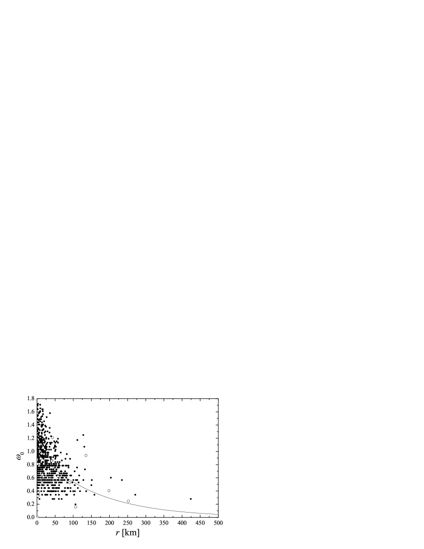
Figure 2: (a) Dependence of the $\omega_{0}$ parameter on the asteroid radius $r$. The solid curve represents exponential approximation (2) with $A_{0}=0.99$, $r_{0}=163$ km. (b) The same as in (a), but with the data on Saturnian satellites (Thomas, 2010) superposed.

Let us recall the notions of these two kinds of synchronous 1:1 resonance, following (Melnikov and Shevchenko, 2000). For a satellite in an eccentric orbit, at definite values of the $\omega_{0}$ inertial parameter, synchronous resonance can have two centres in spin-orbit phase space; in other words, there can be two different synchronous resonances, stable in the planar rotation problem. Consider a section, defined at the orbit pericentre, of the spin-orbit phase space. At $\omega_{0}=0$, there exists a sole centre of synchronous resonance with coordinates $\theta=0\mbox{ mod }\pi$, ${\rm d}\theta/{\rm d}t=1$. If the eccentricity is non-zero, upon increasing the value of $\omega_{0}$, the resonance centre moves down the ${\rm d}\theta/{\rm d}t$ axis, and at a definite value of $\omega_{0}$ another synchronous resonance appears; at small eccentricities this value of $\omega_{0}$ is close to 1, see (Melnikov and Shevchenko, 2000, fig. 2), (Melnikov and Shevchenko, 2008, fig. 3). Following (Melnikov and Shevchenko, 2000), we call the former resonance (emerging at zero value of $\omega_{0}$) the alpha mode, and the latter one — the beta mode of synchronous resonance. Upon increasing the $\omega_{0}$ parameter, the alpha and beta modes coexist over some limited interval of $\omega_{0}$ (the extent of this interval depends on the orbital eccentricity), and in the phase space section there are two distinct resonance centres situated at one and the same value of the satellite’s orientation angle. For illustration see the phase space section in Fig. 5c, given below. Such an effect takes place for Amalthea (J5) (Melnikov and Shevchenko, 1998, 2000); in (Kouprianov and Shevchenko, 2006) the conditions for this effect, called there the “Amalthea effect”, were considered and discussed. On further increasing the $\omega_{0}$ parameter, at some value of $\omega_{0}$ the alpha resonance disappears, i. e., it becomes unstable in the planar problem, and only the beta resonance remains; for illustration see (Melnikov and Shevchenko, 2000, figs. 1 and 2), (Melnikov and Shevchenko, 2008, fig. 3).

3 The ($\omega_{0}$, $r$) relationship

To make inferences on the possible rotational dynamics of a satellite, one should know, in particular, its inertial parameters, generally derived from the three-dimensional form of the satellite. Such information is available now only for a very limited number of satellites (less than 40). So, one has to find ways of estimating these parameters from more available characteristics, e.g, rough estimates of size. Kouprianov and Shevchenko (2006) made exponential and power-law fits to the dependences of the inertial parameters $A/C$ and $B/C$ on the satellite radius $r$, defined as the geometric mean $r=(abc)^{1/3}$ of the semiaxes of the triaxial ellipsoid approximating the shape of the satellite. They found that the exponential fits were better, having greater values of the correlation coefficient. Melnikov and Shevchenko (2007) constructed the dependence of the $\omega_{0}$ parameter on the satellite size (radius) $r$. Following (Kouprianov and Shevchenko, 2006), they fitted the statistical ($\omega_{0}$, $r$) relationship for 34 satellites by an exponential function:

$$\omega_{0}(r)=A_{0}\exp(-r/r_{0}),$$ (3)

and found $A_{0}=0.88\pm 0.07$, $r_{0}=270\pm 65$ km, while the correlation coefficient $R^{2}=0.77$. Fig. 1 shows the derived statistical dependence of the $\omega_{0}$ parameter on the satellite size $r$. Approximation (3) is shown by the solid curve.

Let us apply a simple power-law fit of the form $\omega_{0}(r)=(r/r_{0})^{-p}$ to the same data. This gives $p=0.33\pm 0.06$, $r_{0}=7.22\pm 2.59$ km, and a much smaller value of the correlation coefficient: $R^{2}=0.58$; i.e., the power-law fit is much worse. Also it is worse from the physical viewpoint: an analysis of the expected form of the small satellites (Kouprianov and Shevchenko, 2006) predicts that in the limit $r\to 0$ the $\omega_{0}$ parameter should be $\sim 1$, while the power-law fit gives infinity in this limit; what is more, the decay of the fitting function at large values of $r$ should be fast enough to describe the practically zero values of $\omega_{0}$ for the big satellites, while the power-law fit gives substantially non-zero $\omega_{0}$ values for them.

So, exponential fit (3) is much better and we use it in what follows. Note that we introduce the continuous fit for purely technical purposes, just to predict the $\omega_{0}$ value straightforwardly, solely on the basis of an observational estimate of the radius of a satellite. Does this continuous function have any physical meaning? This depends on whether there is a continuous transition in the shape asymmetry and size from small to large satellites. There is an indication that there is no continuous transition. As delineated in Fig. 1 by two dashed rectangular boxes, the satellites can be roughly divided into two groups: small and irregularly shaped (those with $r<300$ km and $\omega_{0}>0.2$; box A) and big and round (those with $r>500$ km and $\omega_{0}<0.2$; box B). This division is highly distinctive: there are no satellites in the range of radii $r$ from 300 to 500 km. What is more, the two groups are sharply separated in $\omega_{0}$: there are no known small satellites with $\omega_{0}<0.24$ and big satellites with $\omega_{0}>0.21$. Note that, if we consider the primary inertial parameters $A/C$ and $B/C$ instead of $\omega_{0}$, the satellites are not so well separated: the small and big satellites overlap in the values of them, see fig. 3 in (Kouprianov and Shevchenko, 2006).

It is remarkable that the division into two box populations in Fig. 1 does not straightforwardly coincide with any known physical division of the satellites, such as regular–irregular, differentiated–undifferentiated, impact-formed–hydrostatic-equilibrium divisions. Indeed, all satellites in the diagram (in both boxes A and B), except Phoebe in box A and Triton in box B, are regular; see satellite classification and definition of regular and irregular satellites in (Sheppard, 2006). Box A includes both differentiated and undifferentiated and both impact-formed and hydrostatic-equilibrium objects.

Note that, by pointing out the apparent division of the satellites into two separate groups the ($\omega_{0}$, $r$) diagram, we do not try to attach any physical or cosmogonical meaning to this division. In fact, any physical mixture in box A or B, or in the sample as a whole, is not important for our dynamical study, because only the moments of inertia and orbital eccentricity play role in the equations.

Notwithstanding the possible separation of the data into two groups, the continuous description (3) is definitely useful for statistical predictions, as testified by a rather high value of the correlation coefficient and the over-all qualitative agreement with the observed data, including the physically correct behaviour in the limits $r\to 0$ and $r\to\infty$. We do not explore the problem whether the exponential fit has any physical meaning, as redundant for our further dynamical study.

[Figure 1]

[Figure 2]

The fitting law (3) was derived in (Melnikov and Shevchenko, 2007) on the basis of a very limited sample (including only 34 objects), so the problem of its universality remains. We can try to acquire a firmer confidence in it analyzing a similar relationship for asteroids. Indeed, many planetary satellites can be a product of orbital capture of asteroids (Sheppard, 2006; Jewitt and Haghighipour, 2007; Jewitt, 2009). Much greater statistics (though of less quality) are available for asteroids than for satellites, as we demonstrate below. We build the statistical ($\omega_{0}$, $r$) relationship for asteroids in the following way.

Let us rewrite the formula $\omega_{0}=\sqrt{3(B-A)/C}$ in the form

$$\omega_{0}=\sqrt{3\frac{\gamma^{2}-1}{\gamma^{2}+1}},$$ (4)

where $\gamma=a/b$, and $a>b>c$ are the semiaxes of a homogeneous triaxial ellipsoid approximating the form of an asteroid or a satellite. Representation (4), valid for such an ellipsoid, follows from the formulas for the moments of inertia expressed through the semiaxes; see, e.g., (Kouprianov and Shevchenko, 2005). From (4) it follows that 1) $\omega_{0}$ depends only on $a$ and $b$, and does not depend on $c$, 2) the upper limit for $\omega_{0}$ is equal to $\sqrt{3}\approx 1.732$.

The amplitude $\Delta m$ of variation of the stellar magnitude of an asteroid is given by the formula

$$\Delta m=-\frac{5}{4}\log\left(\cos^{2}\varphi+\gamma^{-2}\sin^{2}\varphi\right),$$ (5)

where $\varphi$ is the angle of the spin vector with respect to the line of sight and it is assumed that the asteroids are in a principal-axis rotation state; see (Lacerda and Luu, 2003; Lacerda and Jewitt, 2007; Masiero et al., 2009). Taking instead of $\varphi$ its mean value $\bar{\varphi}$ (equal to 1) over hemisphere and inverting formula (5), one obtains a relation for $\gamma$ through $\Delta m$:

$$\gamma=\sqrt{\frac{\sin^{2}\bar{\varphi}}{10^{-\frac{4}{5}\Delta m}-\cos^{2}\bar{\varphi}}}\ ,$$ (6)

Then it is substituted in formula (4). So, $\omega_{0}$ can be approximately estimated if $\Delta m$ is known.

Taking the tables from (http://www.minorplanetobserver.com/astlc/LightcurveParameters.htm, ) as a source of data on $\Delta m$, in this way we estimate $\omega_{0}$ for 681 asteroids. The data for trans-neptunian objects have been excluded from the sample, since these data are strongly biased to large objects. (What is more, TNOs might be physically irrelevant for comparing with most of the satellites, see Sheppard (2006).) Fig. 2a shows the derived statistical dependence of the $\omega_{0}$ parameter on the asteroid radius $r$. Fitting the dependence by formula (3) gives $A_{0}=0.99\pm 0.02$, $r_{0}=163\pm 15$ km; the correlation coefficient $R^{2}=0.18$. The fitting curve is drawn in the Figure.

Comparing Figs. 1 and 2a, one can see that all asteroids in Fig. 2a except Ceres are situated inside the boundaries of box A of Fig. 1, and none of the asteroids correspond to population in box B. Nevertheless the results of the exponential fitting for the asteroids are very similar to those for the whole sample of satellites. Though, as expected, the correlation coefficient is much less for the asteroidal data, the parameter values are similar, especially in the case of $A_{0}$. Note that $A_{0}=1$ yields a physically justified limit $\omega_{0}=1$ for a small object size: this limit is consistent with the expected axial ratios for a monolithic rock fragment, see discussion in (Kouprianov and Shevchenko, 2006). It is remarkable that such satellites (with $\omega_{0}\approx 1$) in low-eccentricity orbits are subject to the Amalthea effect (see Section 2); so the fitting results predict that this effect should be usual for small planetary satellites in close-to-circular orbits; of course, this concerns only tidally-evolved objects, such as most of small regular satellites and big “particles” of planetary rings.

For our further analysis it is important that the fitting results for the asteroids provide a significant supplementary justification of applicability of relationship (3) for estimating the expected value of $\omega_{0}$, when solely the size of an object is available.

Let us return to the satellites. Up to now, when constructing the ($\omega_{0}$, $r$) diagram, we have used an inhomogeneous sample of objects. The available data for any separate homogeneous sample of objects (e.g., satellites of a separate planet) are too limited for statistical conclusions. However, one can make visual inferences in the case of the Saturnian satellites, where the data are most representative. In Fig. 2b, we superpose the latest data about 17 Saturnian satellites, taken from (Thomas, 2010), on the asteroidal data. We include only box A satellite population, since all (except one) asteroids fit in this box. One can see that the points are even closer to the exponential curve (fitting the asteroidal data) than many asteroids.

4 The ($\omega_{0}$, $e$) diagram

The ($\omega_{0}$, $e$) stability diagram is presented in Fig. 3a. Theoretical boundaries of the zones of existence (i.e., stability in the planar problem) of synchronous resonances are drawn in accordance with (Melnikov, 2001). Regions marked by “Ia” and “Ib” are the domains of sole existence of alpha resonance, “II” is the domain of sole existence of beta resonance, “III” is the domain of coexistence of alpha and beta resonances, “IV” is the domain of coexistence of alpha and period-doubling bifurcation modes of alpha resonance, “V” is the domain of non-existence of any 1:1 synchronous resonance, “VI” is the domain of sole existence of period-doubling bifurcation modes of alpha resonance. Domain V in Fig. 3a is not shaded, so we call it henceforth the “white domain”.

The structure of the diagram in the given ranges of $\omega_{0}$ and $e$ in Fig. 3a is formed by four curves.

At the point $\omega_{0}=1$, $e=0$, the branching curve is born (Zlatoustov et al., 1964; Torzhevskii, 1964). To the left-hand side from the branching curve, only one uneven $2\pi$–periodic solution of the Beletsky equation (alpha resonance) can exist; to the right-hand side, one or two stable solutions (beta resonance or both alpha and beta resonances, respectively) can exist (Zlatoustov et al., 1964; Torzhevskii, 1964). (The synchronous resonance corresponding to the stable uneven $2\pi$–periodic solution existing only for $\omega_{0}\geq 1$ is beta resonance. The synchronous resonance corresponding to a different stable uneven $2\pi$–periodic solution existing both at $\omega_{0}\geq 1$ and at $\omega_{0}<1$ is alpha resonance.)

At the point $\omega_{0}=1/2$, $e=0$, the zone of parametric resonance emerges. (It is “v-shaped” in the vicinity of the point.) The left boundary of this zone corresponds to the loss of stability of the uneven $2\pi$–periodic solution (alpha resonance existing in domain Ia) through the period-doubling bifurcation. This line is the left dashed curve in Fig. 3a. The second (right) dashed curve, drawn in accordance with (Melnikov, 2001), corresponds to the loss of stability of the bifurcated mode through the second consecutive bifurcation. Thus the dashed borders of domains IV and VI are formed by the lines of the first doubling bifurcation (on the left) and the second doubling bifurcation (on the right).

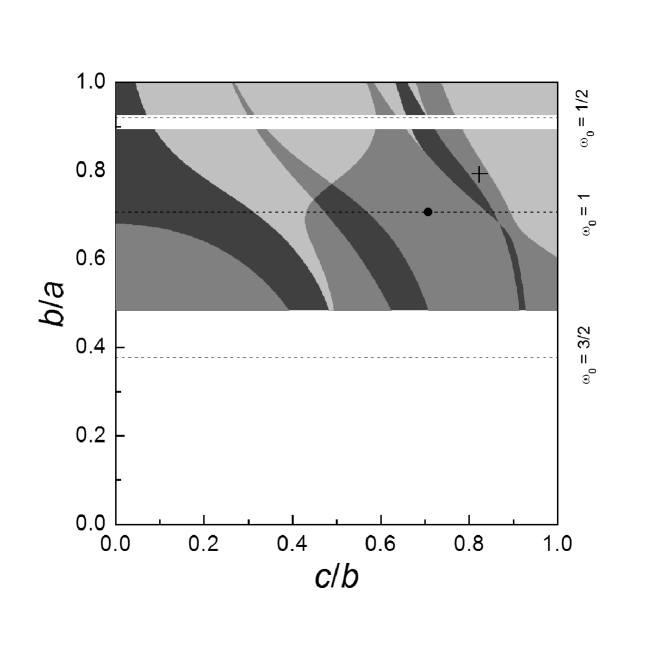
Figure 4: Regions of stability and instability with respect to tilting the axis of rotation; $e=0.1$ (the Hyperion case).

The borders between zones have been found by means of a numerical method of consecutive iterations. It is based on locating the centre of synchronous resonance in the phase space section defined at the pericentre of the orbit. As an initial approximation, one takes the coordinates of the centre of resonance, known beforehand (e.g., at $\omega_{0}=0$ and $e\geq 0$ one has $\theta=0$ and $d\theta/dt=1$ for the centre of synchronous resonance). By solving the Beletsky equation numerically, one finds the maximum deviation (in the phase space section) of the trajectory from the initial data. Taking the half of this deviation, one finds the next approximation for the initial data. The iterative procedure is stopped when the deviation is found to be zero, up to an adopted level of accuracy. On varying the value of $\omega_{0}$ or $e$, the moment of loss of stability (the moment of bifurcation) is fixed, when the consecutive iterations for determining the coordinates of the centre of resonance cease to converge, i.e., when the regular island corresponding to a given kind of synchronous resonance ceases to exist. The obtained locations of the branching curve and the borders of parametric resonance are in agreement with graphs in (Zlatoustov et al., 1964, fig. 4) and (Bruno, 2002, fig. 14), where they were obtained by different semi-analytical methods.

Graphical illustrations of the appearance and locations of various kinds of resonances in phase space sections are given below in Section 6.

[Figure 3]

To place satellites in the diagram, one should know the values of $\omega_{0}$ and $e$. The values of $\omega_{0}$ are available now for 34 satellites only; see compilation and references in (Kouprianov and Shevchenko, 2005). For all other satellites (with unknown values of $\omega_{0}$), following an approach proposed in (Melnikov and Shevchenko, 2007), we estimate $\omega_{0}$ by means of approximation (3) of the observed dependence of $\omega_{0}$ on the satellite size $r$. The data on sizes (and on orbital eccentricities) we take from (Karkoschka, 2003; Sheppard and Jewitt, 2003; Sheppard, Jewitt, and Kleyna, 2005, 2006; Porco et al., 2007; Thomas et al., 2007; http://ssd.jpl.nasa.gov/, ).

In total, the data on sizes and orbital eccentricities are available for 145 satellites. So, there are 145 “observational points” in the ($\omega_{0}$, $e$) stability diagram in Fig. 3a. (Note that, for other purposes, the locations of 10 satellites in the ($\omega_{0}$, $e$) diagram were investigated in (Melnikov, 2001), the position of 13 satellites in this diagram was described in (Bruno, 2002), and the locations of 87 satellites in this diagram were studied in (Melnikov and Shevchenko, 2007).) The solid circles in Fig. 3a represent the satellites with known $\omega_{0}$. The open circles represent the satellites with the $\omega_{0}$ parameter determined by formula (3). The horizontal bars indicate the three-sigma errors in estimating $\omega_{0}$. They are all set to be equal to the limiting maximum value $0.21$, following from the uncertainty in $A_{0}$. This gives an approximate range of the possible values of $\omega_{0}$ at small values of $r$.

From the constructed diagram we find that 73 objects are situated in domain V (“white domain”). In domain Ib, 12 objects are situated above Hyperion (a sole solid circle in domain Ib), while two objects are below Hyperion. No synchronous states of rotation exist in domain V. In the next Section we show that for the majority of the satellites in domain Ib (namely, for the objects above Hyperion) synchronous rotation is highly probable to be attitude unstable. So, 73 objects in domain V and 12 objects in domain Ib rotate either regularly and much faster than synchronously (those tidally unevolved), or chaotically (those tidally evolved). Summing up the objects, we see that a major part (at least 85 objects) of all satellites with unknown rotation states (132 objects), i.e., at least 64 per cent, cannot rotate synchronously.

Note that the exponential (or any other) curve fitting of the ($\omega_{0}$, $r$) dependence is not crucial for achieving the final results of our study. The curve fitting is used here solely on technical reasons. Practically the same results can be achieved without making curve approximations, but basing solely on the division of the sample in the ($\omega_{0}$, $r$) plane into two groups (box A and box B populations). This is demonstrated in Fig. 3b, where the borders of the box A population are superposed on the stability diagram. These borders have been found without making any curve fit, but solely by calculating the $\omega_{0}$ scatter for the objects in box A. The shaded area in Fig. 3b corresponds to the $\omega_{0}$ values in the range $0.68\pm 0.21$. This is the average value of $\omega_{0}$ taken with its $3\sigma$ uncertainty for the satellites in box A in Fig. 1. One can see that this straightforward “projecting” of box A into the ($\omega_{0}$, $e$) diagram predicts location for the satellites with unknown inertial parameters similar to that given by the exponential fitting procedure. However, the latter procedure is definitely better, because it predicts the $\omega_{0}$ value in the limit $r\to 0$, while the former uses the average $\omega_{0}$ value taken at $r$ from 0 to $\approx 250$ km.

5 Attitude stability of synchronous rotation in domain Ib

An analysis of the attitude stability of synchronous rotation allows one to increase the expected number of satellites that cannot rotate synchronously to an even greater value. To demonstrate this, let us consider the attitude stability of the satellites in domain Ib, i.e., the satellites in exact alpha resonance.

The system of equations in variations with respect to the periodic solution in this problem consists of six linear differential equations of the first order with periodic coefficients. (The original system of the Euler equations, describing the three-dimensional rotational motion, is given, e.g., in (Wisdom et al., 1984, eqs. 6). The Euler equations are linearized in the variations; this gives the mentioned linear system.) Numerical integration of the system allows one to obtain the matrix of linear transformation of variations for a period; see (Wisdom et al., 1984). The periodic solutions in the given problem are characterized by three pairs of multipliers. Following (Melnikov and Shevchenko, 2000), we build the distributions of the modules of multipliers for a set of trajectories corresponding to a centre of synchronous resonance on a grid of values of the $b/a$ and $c/b$ parameters. Analysis of the distributions allows one to separate orbits stable with respect to tilting the axis of rotation from those which are attitude unstable (Melnikov and Shevchenko, 2000).

[Figure 4]

The computed regions of stability and instability are shown in Fig. 4 for $e=0.1$ characteristic for the Hyperion case. The regions of stability are represented in light gray, the regions of minimum (one degree of freedom) instability are in dark gray, and the regions of maximum (two degrees of freedom) instability are in black. The white areas in Fig. 4 correspond to case when alpha resonance does not exist. (The intervals of values of $\omega_{0}$, corresponding to the alpha resonance non-existence, can be found from Fig. 3a, where they are given by the extents (in $\omega_{0}$) of domains Ia and Ib at the fixed eccentricity $e=0.1$.) Lines of constant values of the $\omega_{0}$ parameter are drawn in Fig. 4 for reference. The location of Hyperion is shown by a cross; the data on its $a$, $b$, and $c$ are taken from (Black et al., 1995). A bold dot represents the expected location of a satellite with size tending to zero (see Kouprianov and Shevchenko (2006)): $b/c=b/a=0.708$. Both the cross and the dot are apparently situated in regions of instability, which occupy large portions of the area of the diagram. With increasing $e>0.1$, the area of the instability regions only increases, and this means that for the satellites situated in domain Ib above Hyperion there is almost no chance to reside in an attitude-stable rotation state.

There are 15 objects present in domain Ib in Fig. 3a. Twelve of them have orbital eccentricities greater than $0.1$. Therefore one can add these 12 satellites to the total sample of the satellites that are not expected to rotate synchronously.

6 Basic kinds of phase space sections

To provide graphical illustrations to our conclusions, we construct representative phase space sections of the planar rotational motion in the basic domains in the ($\omega_{0}$, $e$) stability diagram. The phase space sections are defined at the pericentre of the orbit; i.e., the motion is mapped each orbital period.

Basic qualitative kinds of the phase space sections, corresponding to domains Ia, Ib, III, and IV, are presented in Fig. 5. For each domain we take a representative satellite. Namely, the sections are constructed for Phoebe (S9) ($e=0.176$, $\omega_{0}=0.365$; thus belonging to domain Ia), Hyperion (S7) ($e=0.100$, $\omega_{0}=0.827$; domain Ib), Amalthea (J5) ($e=0.003$, $\omega_{0}=1.214$; domain III), and Pandora (S17) ($e=0.004$, $\omega_{0}=0.870$; domain IV).

[Figure 5]

In the cases of domains Ia and Ib, the phase space sections contain a broad chaotic layer with alpha resonance inside (Figs. 5a, b). In the case of domain III (Fig. 5c), there exist alpha resonance (the lower one in the section) and beta resonance (the upper one). In the case of domain IV, there exist alpha resonance and its period-doubling bifurcation mode. The latter mode appears as the two islands inside the chaotic layer, to the left and to the right of alpha resonance (Fig. 5d).

[Figure 6]

[Table 1]

A representative phase space section in the case of domain V (“white domain”) is given in Fig. 6. Here we use model values of the parameters, namely, $e=0.25$ and $\omega_{0}=0.9$. They roughly correspond to the centre of the “white domain”. No synchronous state (neither alpha nor beta) exists in the phase space section. There is a prominent chaotic sea instead.

A practical guide for interpretation of details of the phase space sections in Figs. 5 and 6 is provided by Table 1, where prominent regular islands in the sections are identified with resonances.

7 Despinning times

If the orbit is fixed, the planar rotation (i.e., the rotation with the spin axis orthogonal to the orbital plane) in synchronous 1:1 resonance with the orbital motion is the most likely final mode of the long-term tidal evolution of the rotational motion of a planetary satellite (Goldreich and Peale, 1966; Peale, 1969, 1977). In this final mode, the rotational axis of a satellite coincides with the axis of the maximum moment of inertia of the satellite and is orthogonal to the orbital plane. If the orbit exhibits nodal precession, the typical final evolutionary state of the spin axis of a satellite is a low-obliquity Cassini state (Colombo, 1966; Peale, 1969, 1977; Correia, 2009).

Calculation of the time of despinning to synchronous state, due to tidal evolution, shows whether a satellite’s spin could evolve to synchronous state since the formation of the satellite. For a satellite to be ultimately captured in synchronous 1:1 spin state, or any other spin-orbit resonance, the current dynamical and physical properties of the satellite should allow for a sufficiently short, at least less than the age of the Solar system, time interval of tidal despinning to the resonant state.

Let us consider theoretical estimates of the despinning time for the satellites in the “white domain” and domain Ib. We estimate the tidal despinning time of a satellite by means of the following formula (Dobrovolskis, 1995):

$$T_{\mathrm{despin}}=\frac{\omega_{\mathrm{I}}-\omega}{|{\dot{\omega}}|},$$ (7)

where $\omega_{\mathrm{I}}$ and $\omega$ are the initial and the final spin rates of a satellite, respectively, and

$$|{\dot{\omega}}|=\frac{45\rho r^{2}n^{4}}{38\mu Q}$$ (8)

is the absolute value of the rate of the rotation slowdown (see equations (1) and (11) in (Dobrovolskis, 1995)). Here $r$ is the satellite radius, $n=2\pi/T_{\mathrm{orb}}$ is its orbital frequency (the mean motion), $\rho$ and $\mu$ are the density and rigidity of the satellite, respectively; $Q$ is the satellite’s tidal dissipation function. Eq. (8) corresponds to the commonly considered case of the low orbital eccentricities (Dobrovolskis, 1995). In case of the high eccentricities we use formula (4) from (Dobrovolskis, 1995):

$$|{\dot{\omega}}|=(1-e^{2})^{-9/2}\left(1+3e^{2}+\frac{3}{8}e^{4}\right)\frac{45\rho r^{2}n^{4}}{38\mu Q}.$$ (9)

We estimate $T_{\mathrm{despin}}$ for two sets of the values of parameters, namely, the set adopted and justified in (Dobrovolskis, 1995) ($\omega_{\mathrm{I}}=2\pi/(10\;\mathrm{hours})$, $\rho=1\;\mathrm{g}\,\mathrm{cm}^{-3}$, $\mu=3.5\times 10^{10}\;\mathrm{dyn}\,\mathrm{cm}^{-2}$) and the set adopted and justified in (Peale, 1977) ($\omega_{\mathrm{I}}=2\pi/(2.3\;\mathrm{hours})$, $\rho=2\;\mathrm{g}\,\mathrm{cm}^{-3}$, $\mu=5\times 10^{11}\;\mathrm{dyn}\,\mathrm{cm}^{-2}$). The final $\omega$ is fixed to be equal to $2\pi/T_{\mathrm{orb}}$, i. e., the value at synchronous resonance, but note that for any estimates by the order of magnitude the choice of the exact final $\omega$ does not matter much.

The calculation of despinning times for the objects in domains V and Ib shows that the minimum values of these times belong to Elara (J7) with $6\times 10^{12}Q$ years, Carme (J11) with $4\times 10^{13}Q$ years, and Themisto (J18) with $7\times 10^{12}Q$ years. These minimum values are exceeded by typical ones in the set by 2–3 orders of magnitude. Taking $Q\sim 100$ (Peale, 1977), one finds that the despinning times of the satellites in domains V and Ib are by far large in comparison with the Solar system age. The spins of these satellites could not have evolved up to entering the chaotic zone near low order spin-orbit resonances. This is in agreement with the general conclusion by Peale (1977) that most of irregular satellites still remain in spin states close to initial ones.

The irregular satellites can be a product of orbital capture (Sheppard, 2006; Jewitt and Haghighipour, 2007; Jewitt, 2009) or disruption of larger bodies (Colwell, 1994; Sheppard, 2006; Jewitt, 2009). If the objects in domains V and Ib are a product of recent capture or disruption, the allowed times for evolution are even smaller. If most of them originated from capture from the asteroidal population, the spin distribution among the satellites should have remained practically unchanged. Could a captured asteroid have a large enough initial rotation period that allowed immediate entering the chaotic zone?

According to (Pravec and Harris, 2000; Harris and Pravec, 2006), among the asteroids with known rotation periods there exists a statistically distinct (about 2 per cent of the total population) group of “slow rotators” with measured rotation periods up to $\approx 1000$ hours (50 days); an observed lower boundary for the rotation periods of the asteroids in this group is $\approx 30$ hours for the objects with diameter less than 10 km. An even greater excess of slow rotators was found in new surveys by Pravec et al. (2008) and Masiero et al. (2009). Pravec et al. (2008) explain this excess as due to the Yarkovsky effect.

In principle, a satellite with a small enough orbital period, like Themisto (with $T_{\mathrm{orb}}\simeq 130$ d), if it were such an outlier captured in the orbit, could have entered the chaotic zone in phase space. One should take into account that the extent of the chaotic zone, depending on the inertial and orbital parameters, might be rather large in rotation frequency, the upper border being an order of magnitude greater than the synchronous frequency value, see figs. 7–9 in (Dobrovolskis, 1995) and fig. 3 in (Kouprianov and Shevchenko, 2005). However, the chances are apparently low, and one can hardly expect that more than one or two satellites in the “white domain” rotate chaotically, — of course, if one takes for granted that the tidal processes are well understood, and so the real tidal evolution could not be faster. An example provided by Iapetus (S8) shows that there might be situations when the tidal evolution is much faster than in the standard theories: there is an inconsistency of at least two orders of magnitude between the calculated (large) despinning time for this satellite and the observational fact that it is tidally despun (Castillo-Rogez et al., 2007; Aleshkina, 2009). Perhaps a reconsideration of the current tidal despinning theories is needed (Efroimsky and Williams, 2009; Greenberg, 2009). The traditional tidal approach is especially unreliable in the case of highly eccentric and inclined orbits (Greenberg, 2009), i.e., for the irregular satellites. What is more, individual scenarios of orbital evolution for irregular satellites can exist, in which the despinning times are decreased radically, as demonstrated in (Dobrovolskis, 1995) for the case of Nereid (N2), the satellite with the maximum known orbital eccentricity. All these facts, combined with the opportunity of capture of slow rotators, demonstrate that the tidal theory prediction that the current rotation of all irregular satellites is fast might be a subject for revision.

8 Conclusions

On the basis of tidal despinning timescale arguments, Peale showed in 1977 that the majority of irregular satellites are expected to reside close to their initial (fast) rotation states. Here we have investigated the problem of typical rotation states among satellites from a purely dynamical stability viewpoint. We have shown that, though the majority of the planetary satellites with known rotation states rotate synchronously (facing one side towards the planet, like the Moon), a significant part (at least 64 per cent) of all satellites with unknown rotation states cannot rotate synchronously. The reason is that no stable synchronous 1:1 spin-orbit state exists for these bodies, as our analysis of the satellites location in the ($\omega_{0}$, $e$) stability diagram demonstrates. They rotate either regularly and much faster than synchronously (those tidally unevolved) or chaotically (tidally evolved objects or captured slow rotators).

With the advent of new observational tools, more and more satellites are being discovered. Since they are all small, they are all irregularly shaped, according to formula (3). Besides, the newly discovered objects typically move in strongly eccentric orbits (http://ssd.jpl.nasa.gov/, ; Sheppard and Jewitt, 2003). Therefore these new small satellites are all expected to be located mostly in the “white domain” of the ($\omega_{0}$, $e$) stability diagram, i.e., the synchronous 1:1 rotation state is impossible for them.

Table 1

The centres of resonances in the phase space sections

Resonance	Phoebe (S9)	Hyperion (S7)	Amalthea (J5)	Pandora (S17)	Model (Fig. 6)
alpha	$(0,0.940)$	$(0,0.659)$	$(0,0.090)$	$(0,0.976)$	–
beta	–	–	$(0,1.018)$	–	–
period-doubling
alpha	–	–	–	$(\mp 1.302,1.003)$	–
1:2	$(\mp\pi/2,0.589)$	$(\mp\pi/2,0.836)$	–	$(\mp\pi/2,0.784)$	–
5:4	–	–	–	–	$(\mp 0.587,0.957)$
3:2	$(0,1.544)$	–	–	$(0,1.901)$	–
9:4	$(\mp\pi/2,2.182)$,	$(\mp\pi/2,2.000)$,	–	–	–
9:4	$(0,2.319)$	$(0,2.499)$	–	–	–
2:1	$(0,2.063)$	$(0,2.280)$	–	–	–
5:2	–	$(0,2.694)$	–	–	–
7:4	$(\mp\pi/2,1.677)$	–	–	–	–
3:1	–	–	–	–	$(0,3.342)$
7:2	–	–	–	–	$(0,3.782)$
4:1	–	–	–	–	$(0,4.225)$

The numbers in parentheses give the coordinates of the centres of regular islands in Figs. 5 and 6. The “–” symbol signifies that the corresponding mode is absent or is visually unresolved in the section or is situated out of the borders of the graph.

Figure 1: Dependence of the $\omega_{0}$ parameter on the satellite radius $r$ (km). The solid curve represents exponential approximation (2) with $A_{0}=0.88$, $r_{0}=270$ km.

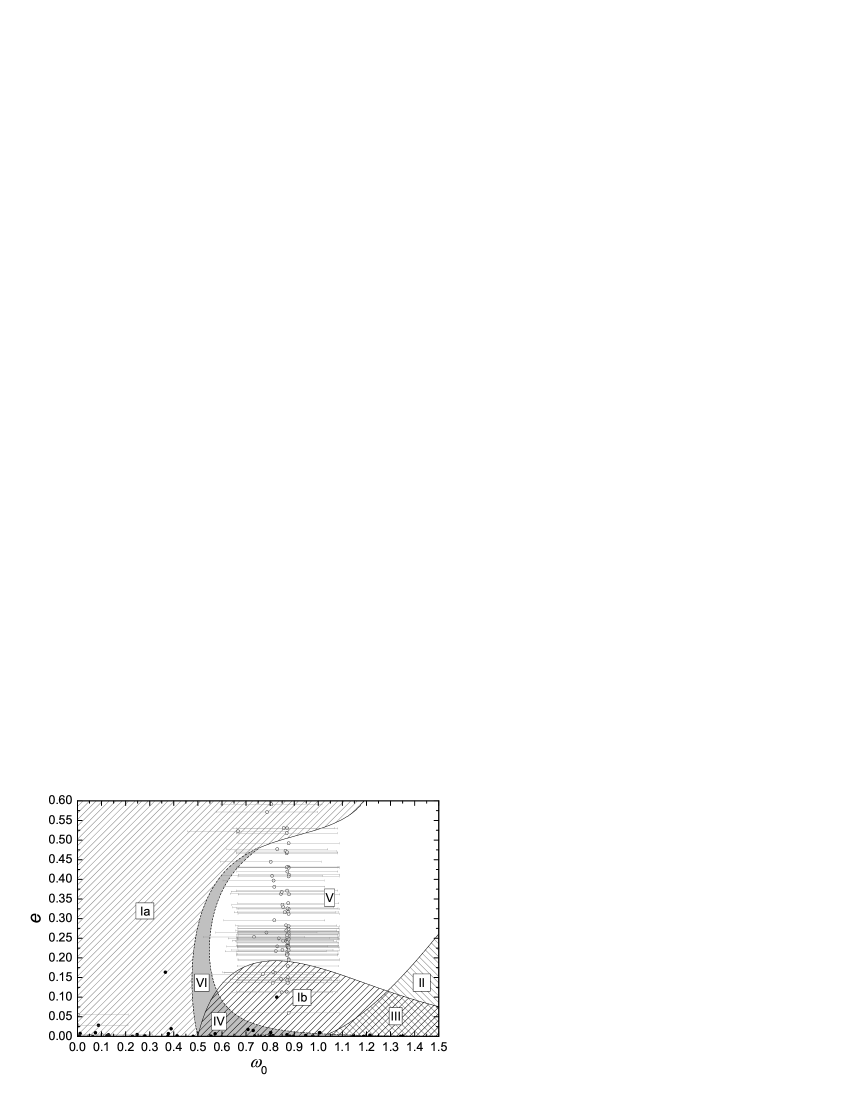
Figure 3: (a) Location of the satellites with known radii in the ($\omega_{0}$, $e$) diagram. (b) Predicted location of the box A population in the same diagram (the shaded area).

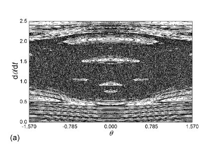
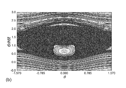
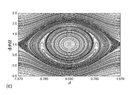
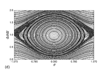
Figure 5: Basic qualitative kinds of the phase space sections for the planar rotational motion. (a) Phoebe (domain Ia), (b) Hyperion (domain Ib), (c) Amalthea (domain III), (d) Pandora (domain IV).

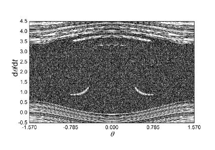
Figure 6: The phase space section for the planar rotational motion of an object in the “white domain”.

References

- Aleshkina (2009) Aleshkina, E.Yu., 2009. Synchronous spin-orbital resonance locking of large planetary satellites. Sol. Sys. Res. 43, 71–78 [Astron. Vestnik 43, 75–82].
- Bauer et al. (2004) Bauer, J.M., Buratti, B.J., Simonelli, D.P., Owen, W.M.Jr., 2004. Recovering the rotational light curve of Phoebe. Astrophys. J. 610, L57–L60.
- Beletsky (1959) Beletsky, V.V., 1959. On libration of a satellite. In: Artificial Satellites of the Earth. Collection of articles, vol. 3. Publishers of the USSR Acad. Sci., Moscow, pp. 13–31. (In Russian.)
- Beletsky (1965) Beletsky, V.V., 1965. The Motion of an Artificial Satellite about its Mass Centre. Nauka Publishers, Moscow. (In Russian.)
- Black et al. (1995) Black, G.J., Nicholson, P.D., Thomas, P.C., 1995. Hyperion: Rotational dynamics. Icarus 117, 149–161.
- Bruno (2002) Bruno, A.D., 2002. Families of periodic solutions to the Beletsky equation. Cosmic Res. 40, 274–295 [Kosmich. Issled. 40, 295–316].
- Castillo-Rogez et al. (2007) Castillo-Rogez, J.C., Matson, D.L., Sotin, C., Johnson, T.V., Lunine, J.I., Thomas, P.C., 2007. Iapetus’ geophysics: Rotation rate, shape, and equatorial ridge. Icarus 190, 179–202.
- Colombo (1966) Colombo, G., 1966. Cassini’s second and third laws. Astrophys. J. 71, 891–896.
- Colwell (1994) Colwell, J.E., 1994. The disruption of planetary satellites and the creation of planetary rings. Planet. Space Sci. 42, 1139–1149.
- Correia (2009) Correia, A.C.M., 2009. Secular evolution of a satellite by tidal effect: Application to Triton. Astrophys. J. 704, L1–L4.
- Devyatkin et al. (2002) Devyatkin, A.V., Gorshanov, D.L., Gritsuk, A.N., Melnikov, A.V., Sidorov, M.Yu., Shevchenko, I.I., 2002. Observations and theoretical analysis of lightcurves of natural satellites of planets. Sol. Sys. Res. 36, 248–259 [Astron. Vestnik 36, 269–281].
- Dobrovolskis (1995) Dobrovolskis, A.R., 1995. Chaotic rotation of Nereid? Icarus 118, 181–198.
- Efroimsky and Williams (2009) Efroimsky, M., Williams, J.G., 2009. Tidal torques: a critical review of some techniques. Celest. Mech. Dyn. Astron. 104, 257–289.
- Goldreich and Peale (1966) Goldreich, P., Peale, S., 1966. Spin-orbit coupling in the Solar system. Astron. J. 71, 425–438.
- Grav et al. (2003) Grav, T., Holman, M.J., Kavelaars, J.J., 2003. The short rotation period of Nereid. Astrophys. J. 591, L71–L74.
- Greenberg (2009) Greenberg, R., 2009. Frequency dependence of tidal Q. Astron. J. 698, L42–L45.
- Harris and Pravec (2006) Harris, A.W., Pravec, P., 2006. Rotational properties of asteroids, comets and TNOs. In: Lazzaro, D., Ferraz-Mello, S., and Fernández, J.A. (Eds.) Proc. IAU Symp. 229. Asteroids, Comets, Meteors. Cambridge University Press, Cambridge, pp. 439–447.
- Jewitt (2009) Jewitt, D., 2009. Six hot topics in planetary astronomy. Lect. Notes Phys., 758, 259–295.
- Jewitt and Haghighipour (2007) Jewitt, D., Haghighipour, N., 2007. Irregular satellites of the planets: products of capture in the early Solar system. Ann. Rev. Astron. Astrophys. 45, 261-295.
- Karkoschka (2003) Karkoschka, E., 2003. Sizes, shapes, and albedos of the inner satellites of Neptune. Icarus 162, 400–407.
- Klavetter (1989) Klavetter, J.J., 1989. Rotation of Hyperion. II — Dynamics. Astron. J. 98, 1946–1947.
- Kouprianov and Shevchenko (2005) Kouprianov, V.V., Shevchenko, I.I., 2005. Rotational dynamics of planetary satellites: A survey of regular and chaotic behavior. Icarus 176, 224–234.
- Kouprianov and Shevchenko (2006) Kouprianov, V.V., Shevchenko, I.I., 2006. The shapes and rotational dynamics of minor planetary satellites. Sol. Sys. Res. 40, 393–399 [Astron. Vestnik 40, 428–435].
- Lacerda and Jewitt (2007) Lacerda, P., Jewitt, D., 2007. Densities of Solar System objects from their rotational light curves. Astron. J. 133, 1393–1408.
- Lacerda and Luu (2003) Lacerda, P., Luu, J., 2003. On the detectability of lightcurves of Kuiper belt objects. Icarus, 161, 174–180.
- Maris et al. (2001) Maris, M., Carraro, G., Cremonese, G., Fulle, M., 2001. Multicolor photometry of the Uranus irregular satellites Sycorax and Caliban. Astron. J. 121, 2800–2803.
- Maris et al. (2007) Maris, M., Carraro, G., Parisi, M.G., 2007. Light curves and colours of the faint Uranian irregular satellites Sycorax, Prospero, Stephano, Setebos, and Trinculo. Astron. Astrophys. 472, 311–219.
- Masiero et al. (2009) Masiero, J., Jedicke, R., Ďurech, J., Gwyn, S., Denneau, L., Larsen, J., 2009. The thousand asteroid light curve survey. Icarus 204, 145–171.
- Melnikov (2001) Melnikov, A.V., 2001. Bifurcation regime of a synchronous resonance in the translational-rotational motion of non-spherical natural satellites of planets. Cosmic Res. 39, 68–77 [Kosmich. Issled. 39, 74–84].
- Melnikov and Shevchenko (1998) Melnikov, A.V., Shevchenko, I.I., 1998. The stability of the rotational motion of non-spherical natural satellites, with respect to tilting the axis of rotation. Sol. Sys. Res. 32, 480–490 [Astron. Vestnik 32, 548–559].
- Melnikov and Shevchenko (2000) Melnikov, A.V., Shevchenko, I.I., 2000. On the stability of the rotational motion of non-spherical natural satellites in synchronous resonance. Sol. Sys. Res. 34, 434–442 [Astron. Vestnik 34, 478–486].
- Melnikov and Shevchenko (2007) Melnikov, A.V., Shevchenko, I.I., 2007. Unusual rotation modes of minor planetary satellites. Sol. Sys. Res., 41, 483–491 [Astron. Vestnik 41, 521–530].
- Melnikov and Shevchenko (2008) Melnikov, A.V., Shevchenko, I.I., 2008. On the rotational dynamics of Prometheus and Pandora. Celest. Mech. Dyn. Astron. 101, 31–47.
- Peale (1969) Peale, S.J., 1969. Generalized Cassini’s laws. Astrophys. J. 74, 483–489.
- Peale (1977) Peale, S.J., 1977. Rotation histories of the natural satellites. In: Burns, J.A. (Ed.) Planetary Satellites. Univ. of Arizona Press, Tucson, pp. 87–111.
- Porco et al. (2007) Porco, C.C., Thomas, P.C., Weiss, J.W., Richardson, D.C., 2007. Saturn s small inner satellites: Clues to their origins. Science 318, 1602–1607.
- Pravec and Harris (2000) Pravec, P., Harris, A.W., 2000. Fast and slow rotation of asteroids. Icarus 148, 12–20.
- Pravec et al. (2008) Pravec, P., Harris, A.W., Vokrouhlický, D., et al., 2008. Spin rate distribution of small asteroids. Icarus 197, 497–504.
- Rauschenbach and Ovchinnikov (1997) Rauschenbach, B.V., Ovchinnikov, M.Yu., 1997. Lectures on the Spaceflight Dynamics. Moscow Physics-Technical Institute, Moscow. (In Russian.)
- Seidelmann et al. (2007) Seidelmann, P.K., Archinal, B.A., A’Hearn, M.F., et al., 2007. Report of the IAU/IAG Working Group on cartographic coordinates and rotational elements: 2006. Celest. Mech. Dyn. Astron. 98, 155–180.
- Sheppard (2006) Sheppard, S.S., 2006. Outer irregular satellites of the planets and their relationship with asteroids, comets and Kuiper Belt objects. In: Lazzaro, D., Ferraz-Mello, S., and Fernández, J.A. (Eds.) Proc. IAU Symp. 229. Asteroids, Comets, Meteors. Cambridge University Press, Cambridge, pp. 319–334.
- Sheppard and Jewitt (2003) Sheppard, S.S., Jewitt, D.C., 2003. An abundant population of small irregular satellites around Jupiter. Nature 423, 261–263.
- Sheppard, Jewitt, and Kleyna (2005) Sheppard, S.S., Jewitt, D., Kleyna, J., 2005. An ultradeep survey for irregular satellites of Uranus: Limits to completeness. Astron. J. 129, 518-525.
- Sheppard, Jewitt, and Kleyna (2006) Sheppard, S.S., Jewitt, D., Kleyna, J., 2006. A survey for “Normal” irregular satellites around Neptune: Limits to completeness. Astron. J. 132, 171–176.
- Thomas et al. (2007) Thomas, P.C., Armstrong, J.W., Asmar, S.W., Burns J.A., Denk T., Giese B., Helfenstein P., Iess L., 2007. Hyperion’s sponge-like appearance. Nature 448, 50–56.
- Thomas (2010) Thomas, P.C., 2010. Sizes, shapes, and derived properties of the Saturnian satellites after the Cassini nominal mission. Icarus, doi: 10.1016/j.icarus.2010.01.025.
- Torzhevskii (1964) Torzhevskii, A.P., 1964. Periodic solutions of the equation of planar librations of a satellite in an elliptic orbit. Kosmicheskie Issledovaniya 2, 667–678. (In Russian.)
- Wisdom (1987) Wisdom, J., 1987. Rotational dynamics of irregularly shaped natural satellites. Astron. J. 94, 1350–1360.
- Wisdom et al. (1984) Wisdom, J., Peale, S.J., Mignard, F., 1984. The chaotic rotation of Hyperion. Icarus 58, 137–152.
- Zlatoustov et al. (1964) Zlatoustov, V.A., Ohotzimskii, D.E., Sarychev, V.A., Torzhevskii, A.P., 1964. Kosmicheskie Issledovaniya 2, 657–666. (In Russian.)
- (51) JPL website data, http://ssd.jpl.nasa.gov/ (Site Manager: D.K.Yeomans.)
- (52) NASA website data, http://solarsystem.nasa.gov/planets/
-
(53)
Collaborative Asteroid Lightcurve
Link (CALL),
http://www.minorplanetobserver.com/astlc/LightcurveParameters.htm/ (Maintained by Harris, A.W., Warner, B.D., and Pravec, P. Version by 2009 April 21.)