The cooling rate of neutron stars after thermonuclear shell flashes

Thermonuclear shell flashes on neutron stars are detected as bright X-ray bursts. Traditionally, their decay is modeled with an exponential function. However, this is not what theory predicts. The expected functional form for luminosities below the Eddington limit, at times when there is no significant nuclear burning, is a power law. We tested the exponential and power-law functional forms against the best data available: bursts measured with the high-throughput Proportional Counter Array (PCA) on board the Rossi X-ray Timing Explorer. We selected a sample of 35 ’clean’ and ordinary (i.e., shorter than a few minutes) bursts from 14 different neutron stars that 1) show a large dynamic range in luminosity, 2) are the least affected by disturbances by the accretion disk and 3) lack prolonged nuclear burning through the rp-process. We find indeed that for every burst a power law is a better description than an exponential function. We also find that the decay index is steep, 1.8 on average, and different for every burst. This may be explained by contributions from degenerate electrons and photons to the specific heat capacity of the ignited layer and by deviations from the Stefan-Boltzmann law due to changes in the opacity with density and temperature. Detailed verification of this explanation yields inconclusive results. While the values for the decay index are consistent, changes of it with the burst time scale, as a proxy of ignition depth, and with time are not supported by model calculations.

1 Introduction

A common phenomenon among mass-transferring low-mass X-ray binaries (LMXBs) with a neutron star (NS) as accretor is a thermonuclear shell flash in the outer layer of that NS (for reviews, see Lewin et al. 1993; Strohmayer & Bildsten 2006). The matter accreted from the companion star is rich in hydrogen and/or helium. It accumulates on the NS in a pile thick enough that, at the bottom, a pressure is reached that is sufficiently high for the ignition of thermonuclear fusion through the CNO cycle and/or triple-$\alpha$ process. The ignition column depth is $y=$10^8-12 g cm^-2, while the geometric depth is $10^{2-4}$ cm, compared to a NS radius of 10⁶ cm. Often, the fusion is unstable and most of the fuel is consumed within a fraction of a second (e.g., Fujimoto et al. 1981; Bildsten 1998). Temperatures reach values in excess of 10⁹ K at the location of ignition. Some of the heat is conducted inward, but most is radiatively transported outward. The photosphere reaches temperatures of order $10^{7}$ K. The thermal emission peaks in the X-ray regime of the spectrum, yielding a ’type I’ (thermonuclear) X-ray burst. Subsequently, the photosphere cools down on a time scale determined by the amount of mass heated up. The deeper the ignition is, the larger the mass heated up and the longer the burst.

It is custom in the literature to model the decay phase of X-ray burst light curves with an exponential function, the light curve being defined as the time history of the number of photons that is detected per unit time (e.g., Lewin et al. 1993; Galloway et al. 2008). The light curve in terms of energy flux is in principle different, because the spectrum changes during the decay as the NS cools. Therefore, the decay rate is not necessarily the same. The difference is not dramatic, though. For the bright phase of X-ray bursts, when the temperature is above 1 keV, the peak of the energy (’$\nu F_{\nu}$’) spectrum is above 3 keV which is for a large part ($>80$%) covered by the bandpass of most X-ray detectors used thus far (2-30 keV).

While exponential decays are generally a good description of the X-ray burst data, this is not based on physical considerations. A simplified derivation of the expected decay law is as follows. Let us assume that the cooling layer has total mass $m$, temperature $T$ and a specific heat capacity at constant pressure of $C_{\rm P}$. Then, the amount of heat is given by

$$Q = m\;C_{P}\;T$$ (1)

If the heat is lost by radiation through a constant area $A$, the rate of loss as a function of time $t$ is given by the Stefan-Boltzmann law:

$$\frac{{\rm d}Q}{{\rm d}t} = -A\sigma_{\rm sb}T_{\rm eff}^{4}=-A\sigma_{\rm sb}{T^{4}\over\tau}$$ (2)

where $\sigma_{\rm sb}$ the Stefan-Boltzmann constant and we assume the layer has optical depth $\tau\gg 1$ with $\tau$ independent of temperature. If heat is promptly transported within the reservoir before being radiated through the photosphere and if the specific heat capacity is independent of temperature, then

$$T = \left(\frac{3A\sigma_{\rm sb}}{m\;C_{P}\tau}\,t\right)^{-1/3}$$ (3)

and

$$L = -\frac{{\rm d}Q}{{\rm d}t}\propto T^{4}\propto t^{-4/3}$$ (4)

with $L$ the bolometric luminosity. Thus, the decay follows a power law. This relationship is unaffected by General Relativity effects close to the neutron star surface.

A more sophisticated study of NS cooling was performed by Cumming & Macbeth (2004), for X-ray bursts with large ignition depths (carbon-fueled ’superbursts’ with durations of roughly half a day), using a multizone model that takes into account the heat transport inside the reservoir after the flash. This study predicts the same 4/3 power-law decay index for late times in the burst, after the cooling wave from the photosphere reaches the ignition depth. We will see later (§4) that the decay index may be different after shallower ignitions.

We decided to verify the theory by checking whether a power law is more consistent with the decay of X-ray bursts than an exponential function, both in photon count rate and energy flux (or $L$). Our study focuses on ’ordinary’ X-ray bursts with durations of a few minutes or less, because those are much more abundant and provide better test data than long bursts. In §2 we explain how we selected and prepared the data for this test, in §3 we present details of the analysis method and results, and in §4 these results are discussed.

2 Data

2.1 Observations

The best data currently available are those collected with the Proportional Counter Array (PCA; Jahoda et al. 2006) on the Rossi X-ray Timing Explorer (RXTE; Bradt et al. 1993) between 1996 and 2012. The PCA consists of 5 Proportional Counter Units (PCUs) with a spectral resolution of 1 keV at 6 keV (full-width at half maximum), a bandpass of 2 to 60 keV and a combined photon-collecting area of about 6500 cm². This implies a typical X-ray burst peak photon count rate of $10^{4}$ s^-1 (for 5 active PCUs) - the highest for any historical X-ray telescope. During the course of the mission the average number of active PCUs decreased, so that in general peak count rates were higher earlier on in the mission. The PCA could simultaneously be read out in 6 different data modes. For our analysis, we depend on ’event mode data’ (few to tens of ms readout resolution, 64 channels between 2 and 60 keV, PCUs unresolved), standard-1 data (0.125 s resolution, no energy resolution, PCUs resolved) and standard-2 data (16 s resolution, 129 energy channels, PCUs resolved).

Galloway et al. (2008) published a catalog of 1187 X-ray bursts detected with the PCA up to 2006. A final catalog is being generated as part of the Multi-INstrument Burst ARchive effort (’MINBAR’) to create an archive of more than 6000 type I X-ray bursts detected with the PCA and instruments on BeppoSAX and INTEGRAL (Galloway et al. 2010). That final catalog covers the complete mission and includes 2097 PCA-detected X-ray bursts plus two superbursts from 59 low-mass X-ray binaries. These burst identifications are the starting point of our study.

2.2 Data selection

Care has to be taken to obtain an unimpeded clean view of the NS cooling process, because the signal may easily be confused by prolonged nuclear burning through the rp process (e.g., Wallace & Woosley 1981; Hanawa & Fujimoto 1984; Woosley et al. 2004; Fisker et al. 2008), scattering or obscuration in the accretion disk or accretion disk corona (e.g., in ’t Zand et al. 2011; Bagnoli et al. 2013) and a varying accretion rate (e.g., Worpel et al. 2013). Therefore, X-ray bursts have to be carefully selected. Light curves were generated of all 2099 bursts. These are histories of the count rate of detected photons as a function of time. PCA ’standard-1’ data were employed for this purpose with a time resolution of 1 s, combining the signal of all active PCUs and photon energies.

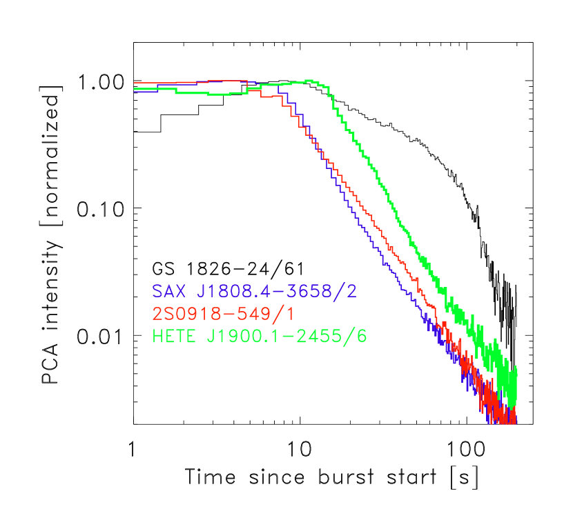
Figure 1: Normalized light curves of three bursts of our sample (c.f., Table 1) and one from GS 1826-24 which has a strong additive component and whose tail cannot be due to cooling alone. The color version of this figure is only available online.

Visual inspection of the burst light curves resulted in the identification of 14 different classes of decay shapes. We are interested in bursts whose measurements are the least affected by strong and variable non-burst emission or by variability that indicates possible disturbances of the accretion flow (e.g., in ’t Zand et al. 2011). Two classes contain bursts with the desired shape of the decay: a smooth curve after a sharp peak or after a broad less defined peak. Bursts in other classes show dents in the decay, have other pre-burst fluxes than post-burst, show rise times similar to their decay times or show multiple peaks without a quiescent period in between.

The first class of smooth decays after sharp peaks is the largest with 655 bursts. That with smooth decays after broad peaks contains 119 bursts. The total of 774 bursts encompass more than one third of all RXTE bursts. Of the other classes, that with bursts with a shoulder shape (see below) is largest (337 bursts). That with bursts with a triangular shape is the least prominent with 7 bursts. It should be noted that 405 bursts were weak and barely rose above the noise. The many bursts from IGR J17480-2446 (Linares et al. 2011) are good examples of that.

To illustrate the difference between smooth and other decays, we show in Fig. 1 a burst with a shoulder shape from GS 1826-24 together with 3 bursts that we ended up selecting. Obviously, the time profile of the burst from GS 1826-24 is rather different and is neither consistent with a pure power law or an exponential function. There is clearly an additional component which lasts 100 s and then drops very fast. Such a burst tail cannot solely be due to cooling. Bildsten (2000) proposed that the shoulder in GS 1826-24 is due to prolonged nuclear hydrogen burning through the relatively slow rp-process. Heger et al. (2007) convincingly proved this by detailed modeling of the nuclear burning.

Figure 2: Cumulative distribution of peak-to-pre-burst flux ratios

Next, an additional selection criterion was applied. The best bursts to study are those with the largest dynamic range in flux, the range being defined as the ratio between the peak and the pre-burst fluxes, because that avoids most of the confusion with changes in accretion flux. The pre-burst flux was calculated by taking the average of the flux in the 20 to 100 s time frame immediately prior to the burst start time as determined by Galloway et al. (2008). The peak flux was determined from the maximum between 10 s prior to 50 s posterior to the burst start, at a time resolution of 1 s. The ratio $R$ is the dynamic range. Fig. 2 shows the cumulative distribution of $R$. To obtain a reasonably sized set of bursts with accurate enough determinations of burst time scale parameters, we initially applied a threshold of $R=50$. This yields 22 bursts from the first class and 8 bursts from the second class (see above). However, seven bursts are from the eclipsing system EXO 0748-676 and were removed because of a high likelihood for interference by the accretion disk due to the high inclination angle (Parmar et al. 1986). Furthermore, we had to leave out 4 bursts for which no event mode or burst catcher data are available. This selection step, going from 755 to 19 bursts is the most restrictive. We note that this does not introduce a selection effect on shape.

To extend the diversity of NSs and bursts, we added bursts with smaller $R$ as well as two long bursts. For the first addition, we searched for LMXBs that had bursts with $R>10$ and picked 2 bursts per LMXBs that were as far apart in time as possible to probe different circumstances. This yielded 14 more bursts from 7 LMXBs. For the addition of long bursts, there is not much choice in the PCA sample (4 bursts). We added an intermediate duration burst from 2S 0918-549 (in ’t Zand et al. 2011) and a superburst from 4U 1636-536 (Strohmayer & Markwardt 2002; Kuulkers et al. 2004; Cumming et al. 2006, Keek et al. in prep.). These two bursts do not have monotonic decays and have low $R$, see §2.3, but particularly the superburst from 4U 1636-536 has the best data available for such a long event.

Our total burst sample consists of 35 ordinary and 2 long bursts from 14 LMXBs, see Table 1. This includes a variety of LMXBs. There are 3 confirmed ultracompact X-ray binaries with presumably a deficiency in hydrogen (4U 0512-40, 2S 0918-549 and 4U 1820-30), 3 accretion-powered X-ray pulsars (IGR J17511-3057, SAX J1808.4-3658 and HETE J1900.1-2455) and 6 transients (4U 1608-52, IGR J17511-3057, SAX J1808.4-3658, XTE J1810-189, HETE J1900.1-2455 and Aql X-1). The rise time of all 37 bursts is fast: the time to rise to 75% of the burst peak count rate is always less than 2 s. This automatically selects flashes of ’pure’ helium layers. Such layers exist either in a H-rich LMXB when the accretion rate is in a favorable regime (e.g., Fujimoto et al. 1981) or in a H-poor LMXB in an ultracompact X-ray binary system with a hydrogen-deficient companion/donor star. 29 out of the 37 bursts are Eddington-limited (see Table 1).

2.3 Data preparation

For each burst we prepared two types of light curves. The first is the history of the photon count rate in the detector. This is the same kind of data that was used for the above data selection. We subtracted for each burst the count rate as determined in a time frame of 20 to 100 s prior to the burst start time.

The second type of light curve is the history of the bolometric flux. This involved a more elaborate data treatment. We employed event-mode data, again combining all active PCUs, but resolved in photon energy. In a few bursts (from 4U 1608-52, 4U 1728-34 and SAX J1808.4-3658) the on-board buffer sometimes overflowed resulting in data stretches not being downloaded and lost. That always happened prior to the cooling phase and does not affect our analysis. We selected calibrated data between 3 and 20 keV that are usually covered by 23 energy channels. First, we generated a spectrum from pre-burst standard-2 data as far as possible (up to 2500 s) and as far as it is anticipated to be representative for the non-burst radiation during the burst (i.e., with a flux that is identical within the noise to the flux immediately prior to the burst). This spectrum was fitted, in Xspec (Arnaud 1996) version 12.8.0d, with a combination of a disk black body (e.g., Mitsuda et al. 1984) and a power law, absorbed following the model by Morrison & McCammon (1983) for cosmic abundances and with hydrogen column densities $N_{\rm H}$ fixed at values obtained from the literature for each source (see Appendix A in Worpel et al. 2013). A systematic error of 0.5% was added quadratically to the statistical error per channel. For the vast majority of spectra this results in an acceptable goodness of fit as measured through $\chi^{2}_{\nu}$. In incidental cases $\chi^{2}_{\nu}$ was formally not acceptable but the effect of that in our analysis was found to be negligible due to the dominance of the burst flux over the persistent flux. Second, the burst was divided in a number of time intervals for which separate spectra were generated from event mode data. These were modeled with a combination of the model for the pre-burst data and a Planck function with a temperature $T{\rm c}$ and a normalization $R^{2}_{\rm 10\leavevmode\nobreak\ kpc}$ where $R_{\rm 10\leavevmode\nobreak\ kpc}$ is the radius of an assumed spherical emission area in km for a distance of 10 kpc. All burst spectra were again multiplied with the same absorption model and fixed hydrogen column density $N_{\rm H}$ as above. Subsequently, the bolometric flux $F$ per burst time interval was determined through the law of Stefan-Boltzmann:

$$F(t)=\sigma_{\rm sb}4\pi R^{2}_{\rm 10\leavevmode\nobreak\ kpc}/(10\leavevmode\nobreak\ {\rm kpc})^{2}T{\rm c}^{4}\leavevmode\nobreak\ \hskip 28.45274pt{\rm erg\leavevmode\nobreak\ cm}^{-2}\leavevmode\nobreak\ {\rm s}^{-1},$$ (5)

where it is assumed that the emitting area is constant. Statistical errors for the bolometric flux were calculated through the same law, by sampling parameter space 10,000 times in (-4$\sigma$,+4$\sigma$) intervals ($\sigma$ representing the single-parameter 1-sigma error) around the best-fit values of k$T_{\rm c}$ and $R^{2}_{\rm 10\leavevmode\nobreak\ kpc}$, searching for all parameter pairs for which $\chi^{2}<\chi^{2}_{\rm min}+2.3$, calculating for those pairs the bolometric flux and searching the minimum and maximum flux values for that $\chi^{2}$ constraint. These delimit the 68% error margin in flux for two free parameters (e.g., Lampton et al. 1976).

The two long bursts (2S 0918-549/5 and 4U 1636-536/sb) involve additional data preparation. Both bursts do not have monotonic decays. The intermediate duration burst from 2S 0918-549 has strong modulations on its decay which extend from 105 to 201 s after the start of the burst (in ’t Zand et al. 2011). We excluded data for this time frame, leaving a few data points between 100 and 105 and between 201 and 226 s. The superburst from 4U 1636-536 has a very low $R$ value of 5.2 and we are forced to exclude a large part of the tail. Furthermore, the cooling wave takes a long time to reach the ignition depth, implying that it is necessary to exclude the first 3000 s of the burst. The left-over data covers 4708 to 8616 s after the start of the burst, compared to a data set extending 20,000 s (including data gaps).

Instrumental dead time corrections were applied to both the bolometric flux values and the photon count rate values.

3 Light curve modeling

We tested two models for the evolution of the flux during the X-ray burst decay. The first is the traditional exponential function:

$$F(t) = F_{0}\;\;e^{-(t-t_{0})/\tau}+F_{\rm bg},$$ (6)

and the second the power law function

$$F(t) = F_{0}\left(\frac{t-t_{s}}{t_{0}-t_{s}}\right)^{-\alpha}+F_{\rm bg}$$ (7)

where $t$ is time, $t_{0}$ the time where $F_{0}$ is measured and $t_{s}$ the time when the cooling starts (irrelevant for the exponential function). $\tau$ is the exponential decay folding time and $\alpha$ the power-law decay index. $F_{\rm bg}$ is the background flux (i.e., everything unrelated to the burst emission and assumed to be constant). It is fixed at 0 for all fits (but see below). $t_{0}$ is chosen to be the time of the first data point included in the fit. The typical burst time scale is $\tau$ for the exponential function and $t_{0}-t_{s}$ for the power law, if $t_{0}$ is the time when the decay starts.

Table 1: Fit results on 35 ordinary bursts and 2 long bursts (at the bottom, below the line). The bursts numbers (column 2) are those from the burst catalog partly published in Galloway et al. (2008). Uncertainties are only provided for $\alpha$ since only power-law fits are acceptable. Sometimes 2 values for $\chi^{2}_{\nu}$ are provided. The fitted values for $\alpha$ apply to the low value of $\chi^{2}_{\nu}$ (see text).

Object	Bu.	MJD	$R$	Photon count rate history				Bol. flux history
	No.			Exponential		Power law		Exponential		Power law
				$\tau$	$\chi^{2}_{\nu}$	$\alpha$	$\chi^{2}_{\nu}$	$\tau$	$\chi^{2}_{\nu}$	$\alpha$	$\chi^{2}_{\nu}$
4U 0512-40*	2	51324.286947	22.3	13.8	3.0	$1.707\pm 0.018$	1.15	$7.9$	14.3	$1.439\pm 0.022$	0.38
4U 0512-40*	15	54839.516222	27.7	11.4	2.5	$1.715\pm 0.024$	0.97	$7.7$	7.1	$1.792\pm 0.042$	0.65
2S 0918-549	1	51676.826588	122.6	19.2	17.7	$1.902\pm 0.007$	1.41	$13.8$	65.9	$1.832\pm 0.013$	1.69
4U 1608-52	8	50914.274663	86.9	14.7	90.2	$1.894\pm 0.004$	1.08	$14.5$	114.9	$1.808\pm 0.016$	1.74/8.31
4U 1608-52	9	51612.030846	59.5	10.1	63.2	$1.829\pm 0.004$	1.49	$3.8$	1.2	$2.141\pm 0.049$	2.45
4U 1608-52	10	51614.071258	111.5	14.0	103.5	$1.995\pm 0.003$	0.95	$9.9$	248.8	$2.000\pm 0.013$	1.05/8.86
4U 1608-52	31	53104.407932	90.7	17.8	64.5	$1.859\pm 0.004$	5.14	$13.0$	256.9	$1.869\pm 0.015$	2.13/9.52
4U 1636-536	68	52286.054034	35.5	9.2	10.2	$1.681\pm 0.010$	1.34	$4.9$	82.6	$1.652\pm 0.011$	2.45
4U 1636-536	327	55394.904042	31.2	12.1	4.9	$1.681\pm 0.016$	1.06	$5.2$	43.7	$1.592\pm 0.014$	1.67
4U 1702-429*	13	51939.193940	42.9	12.5	12.6	$1.816\pm 0.009$	1.17	$6.1$	82.8	$1.751\pm 0.009$	2.02
4U 1702-429	44	53212.793589	43.6	12.0	33.4	$1.825\pm 0.006$	1.43	$7.8$	106.2	$1.874\pm 0.012$	1.81/3.00
4U 1705-44*	51	54046.201890	33.9	12.4	4.4	$1.863\pm 0.017$	1.46	$9.4$	17.9	$1.801\pm 0.021$	0.79
4U 1705-44*	77	55062.220583	29.8	11.4	2.7	$1.807\pm 0.025$	1.05	$5.7$	19.7	$1.421\pm 0.017$	0.68
4U 1724-30	2	53058.401400	16.9	11.4	3.0	$1.823\pm 0.028$	0.96	$4.6$	28.5	$1.651\pm 0.018$	0.99
4U 1724-30	3	53147.218284	27.8	12.9	11.5	$1.764\pm 0.014$	1.31	$5.4$	71.1	$1.857\pm 0.012$	1.19
4U 1728-34	76	51657.203264	33.0	8.1	93.1	$1.786\pm 0.006$	2.19	$6.7$	76.1	$1.781\pm 0.011$	1.18
4U 1728-34	126	54120.25887	29.6	7.6	68.4	$1.784\pm 0.007$	2.02	$6.4$	67.0	$1.835\pm 0.010$	1.00
IGR J17511-3057*	10	55099.313613	43.3	12.4	3.9	$2.303\pm 0.026$	1.09	$10.2$	14.2	$2.320\pm 0.033$	1.89
IGR J17511-3057*	12	55101.289836	47.4	12.4	3.6	$2.134\pm 0.028$	1.40	$9.8$	7.9	$2.065\pm 0.031$	2.05
SAX J1808.4-3658	2	52564.305146	63.8	25.2	13.8	$1.820\pm 0.010$	1.57	$20.4$	32.6	$1.789\pm 0.023$	1.27
SAX J1808.4-3658	3	52565.184268	74.8	24.9	27.0	$1.896\pm 0.008$	2.39	$22.0$	50.3	$1.814\pm 0.050$	0.88/6.50
SAX J1808.4-3658	4	52566.426770	82.8	27.0	22.9	$1.984\pm 0.008$	1.93	$17.0$	113.1	$1.961\pm 0.033$	1.75/9.30
SAX J1808.4-3658	6	53526.638240	76.5	29.1	18.6	$1.868\pm 0.010$	2.20	$17.0$	71.6	$1.954\pm 0.048$	0.67/6.27
SAX J1808.4-3658	7	54732.708128	95.0	30.2	8.2	$2.089\pm 0.017$	1.78	$16.4$	53.3	$2.231\pm 0.041$	2.67/8.13
SAX J1808.4-3658	9	55873.916348	79.7	25.3	24.1	$1.903\pm 0.008$	1.45	$19.1$	40.8	$1.739\pm 0.029$	4.22/10.34
SAX J1810.8-2609	3	54590.729819	62.5	11.2	13.6	$1.833\pm 0.010$	1.14	$11.6$	9.2	$1.633\pm 0.029$	1.24
4U 1820-30	5	53277.438562	13.3	6.4	5.4	$2.002\pm 0.016$	3.33	$5.4$	25.5	$1.991\pm 0.020$	0.75
4U 1820-30	12	54981.187286	15.1	5.2	14.3	$1.901\pm 0.011$	5.28	$7.2$	27.0	$1.885\pm 0.021$	2.09
HETE J1900.1-2455	3	54506.856149	56.1	11.4	30.3	$2.155\pm 0.007$	3.22	$7.9$	100.9	$2.276\pm 0.015$	1.74/3.01
HETE J1900.1-2455	5	54925.796423	72.2	14.7	16.5	$1.858\pm 0.008$	1.31	$9.8$	46.6	$1.727\pm 0.015$	1.77
HETE J1900.1-2455	6	55384.878220	86.5	14.7	38.2	$2.216\pm 0.007$	2.99	$9.3$	137.4	$2.404\pm 0.015$	6.31/11.16
HETE J1900.1-2455	7	55459.228637	59.3	11.3	50.1	$2.234\pm 0.005$	3.59	$9.3$	201.6	$2.289\pm 0.014$	3.71/11.09
Aql X-1	11	51336.590743	64.8	11.0	25.8	$1.802\pm 0.007$	1.18	$12.3$	14.2	$1.531\pm 0.027$	1.73
Aql X-1	25	52100.799520	56.2	8.5	45.5	$1.836\pm 0.005$	1.25	$14.5$	14.3	$1.641\pm 0.026$	1.01
Aql X-1	64	54259.247877	162.5	24.6	67.7	$2.078\pm 0.004$	2.56	$21.6$	108.3	$1.904\pm 0.044$	0.26/6.64
2S 0918-549	5	54504.126944	158.8	110.6	3.4	$1.372\pm 0.007$	1.79	$99.3$	3.9	$1.516\pm 0.005$	1.47
4U 1636-536*	sb	51962.702961	5.2	4387.1	1.5	$1.428\pm 0.004$	1.23	$4879$	5.0	$1.321\pm 0.004$	1.59

* non-PRE burst

Fitting the exponential function to the data involves finding the best values for $\tau$, $F_{0}$ and $F_{\rm bg}$. Fitting the power law involves 4 instead of 3 parameters: $\alpha$, $F_{0}$, $F_{\rm bg}$ and $t_{s}$. In principle one expects $t_{s}$ to be close to the start time of the burst. In both cases we determined $F_{\rm bg}$ from pre-burst data, assuming that during the burst this is not different, see §2.3.

There is a fundamental difference between both functions. The power law is, for positive $\alpha$, divergent for $t=t_{\rm s}$ while the exponential function has no divergence point. That causes a strong coupling between $\alpha$ and $t_{\rm s}$ (e.g., Clauset et al. 2009). Since $t_{\rm s}$ is outside the range of $t$ for which there are data, this may induce a large error on $\alpha$. We work on the presumption that $t_{\rm s}$ is accurately given by the burst start time, but have to keep in mind that on rare occasions this may not be known. Some superexpansion bursts have precursors that are quite short - of order tens of ms (in ’t Zand & Weinberg 2010; in ’t Zand et al. 2011). Fortunately, the PCA instrument is quite sensitive and can pick up small signals, but if precursors are as short as a few ms, that may even be a problem for the PCA. In that case $t_{\rm s}$ may be off by order 1 s. We did vary $t_{\rm s}$ for our bursts, to check whether better fits were possible for start times very different from that of burst onset, but were unable to find such instances (see Fig. 3 for such exercises on bursts from 2S 0918-549 and SAX J1808.4-3658).

Figure 3: Contours of goodness of fit $\chi^{2}_{\nu}$ for a power-law fit to the bolometric flux data for the burst from 0918-549 (upper plot) and burst number 2 from SAX J1808.4-3658 (lower) as a function of $t_{\rm s}$ and $\alpha$. Three contours are drawn, for $\chi^{2}_{\rm min}+\Delta\chi^{2}$ with $\Delta\chi^{2}=1.0,2.3$ and 4.6 (i.e., not per degree of freedom). The first contour delimits the single parameter 1$\sigma$ region. The second and third contour delimit the 68% and 90% confidence regions. The contours show a coupling between both parameters.

It is necessary to skip the first part of the burst, because that is not smoothly decaying yet. For each burst we increased $t_{0}$ from immediately after the peak until $\chi^{2}_{\nu}$ did not decrease anymore. This usually implies that the first 10 s of the burst, including the rising part, are skipped and the flux decreased by approximately a factor of 2. This ensures exclusion of that part of the burst where possibly nuclear burning is ongoing or where the flux is close to the Eddington limit during which part of the radiated energy may be transformed to kinetic and potential energy instead of radiation.

Similarly, it is sensible to not include all data beyond $t_{0}$ but to stop when the burst flux becomes of the same order of magnitude as the pre-burst flux. We did this for the fits to the bolometric flux data. For the photon count rate data we mostly included all data until 200 s after burst onset and longer for the long bursts. Since the data preparation is in this case more straightforward, we thought it interesting to study the decay further down in the tail. This did not result in more insight, though. Inconsistent power law fits are mostly due to random changes in slopes (i.e., shallow to steep and vice versa). We note that, for both sets of data, we used the same data for the fits with the exponential function as for those with the power law.

Table 1 presents the results of the modeling of the photon count rate and bolometric flux data of the 37 selected bursts. Comparing the goodness-of-fits $\chi^{2}_{\nu}$ of the exponential and power-law fits, it is clear that power laws are, for every burst, a better description of both the photon count rate and the bolometric flux data.

In 13 bursts, fitting the power-law function to the bolometric fluxes yields unacceptable values for the goodness-of-fit $\chi^{2}_{\nu}$, although better than for the exponential model. That is probably due to the fact that some spectra in those time series have large values for $\chi^{2}_{\nu}$. In order to obtain more reliable estimates of the uncertainty in the decay index, we multiplied in these cases the errors on flux per time bin with $\sqrt{\chi^{2}_{\nu}}$ of the appropriate spectral fit to force $\chi^{2}_{\nu}$ to 1 and performed the power-law fit again and determine the uncertainty in $\alpha$. For reference, the $\chi^{2}_{\nu}$ values before and after this procedure are provided in Table 1 (last column). There is always considerable improvement in $\chi^{2}_{\nu}$ in the power law fits. The reason why the spectra are formally inconsistent with a black body is unclear. It may be related to transient scattering effects in the accretion flow. If so, then these bursts should, according to our selection requirements not be included in our sample. Therefore, these bursts should be considered with caution.

Figure 4 shows for a representative subset of all bursts the power-law fits to the bolometric flux data.

Figure 4: Power-law fits to bolometric flux histories of 16 representative bursts from 14 different LMXBs. The X-axis represents time since burst onset. There are two panels per burst. The upper panels show the bolometric flux in units of the Eddington flux, as determined from the highest peak flux over all bursts observed per source. The lower panels show the deviation with respect to the model in units of $\sigma$ per data point. All axes of the upper panels and time have an identical dynamic ranges so that slopes can be directly compared. The burst are identified in a slightly abbreviated but straightforward manner (c.f., Table 1). The last two bursts were added to extend the time range, although they do not have smooth decays.

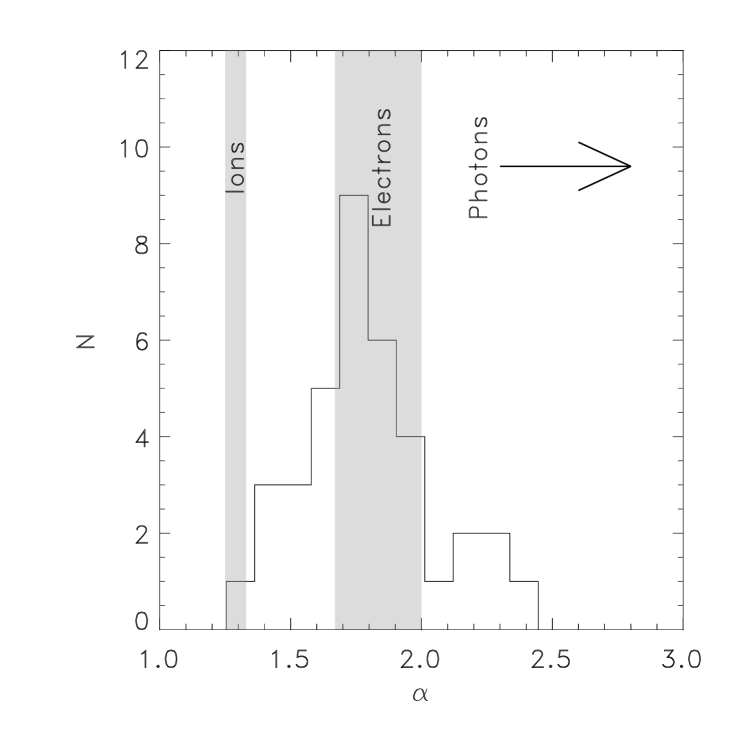
Figure 5: Histogram of power-law decay index of fits to to bolometric flux history of all 37 bursts. The gray areas indicate the canonical values for a pure ideal ion gas (1.25-1.33; see text) and a pure degenerate electron gas (1.67-2.00). When the photons contribute significantly to the heat capacity, $\alpha$ can become higher.

We verified the robustness of the power-law fits to the photon count rate data in order to obtain a sense of the possible systematic errors of the power-law decay index. This verification encompassed 3 tests: how does the power law change when leaving free $F_{\rm bg}$, when limiting the data to fluxes that are 2% or higher than the peak flux, or when both these tests were applied at the same time. We find that individual values of the decay index change on average by 3 to 4% and that the mean value over all bursts changes by only 0.2%. Therefore, the result seems robust.

Concentrating on the power-law fits to the bolometric flux histories of the 35 ordinary bursts, we find that the power-law decay index lies between 1.4 and 2.4, with a weight average of $1.844$ and a standard deviation of 0.24. This is a 0.511 steeper index than the derived value in §1 (4/3). The histogram (Fig. 5) looks bimodal with a primary distribution between $\alpha=1.4$ and 2.1 peaking at $\alpha\approx 1.75$ and a tail of 5 bursts with $\alpha>2.1$. The weight averages of the 4 objects with multiple bursts are: $1.71\pm 0.11$ for 4U 1608-52, $1.87\pm 0.16$ for SAX J1808.4-3658, $2.18\pm 0.26$ for HETE J1900.1-2455 and $1.64\pm 0.16$ for Aql X-1. Due to the large uncertainties (these are the standard deviations), there is no strong evidence for systematic differences between objects. The decay index for the two long bursts is low. That of the superburst is the only one consistent with the canonical 4/3 value.

If we exclude the 13 bursts that we took under reserve in Sect. 3, then the average over the 22 ordinary bursts is $\alpha=1.75\pm 0.21$. This average is only marginally shallower and still 0.418 steeper than 4/3. The range of $\alpha$ also remains similar: 1.4–2.3. Comparing H-rich against H-poor accretors we find 1.86$\pm$0.26 against 1.81$\pm$0.15, which is an insignificant difference.

Many of the power-law fits to the photon count rate data are of good quality as well, with a weighted average of the power-law decay index of $1.929$, which is only 0.085 different from the value for the bolometric flux, and a standard deviation of 0.16 - smaller than for the bolometric flux. On a burst-by-burst basis, the difference is larger than 0.1 seven times, most notably in 4U0512-40/2, 4U 1705-44/77 (these are the two ordinary bursts with the shallowest power-law decay index in bolometric flux), 4U 1608-52/9 and Aql X-1/11.

4 Discussion

For 35 ordinary ’clean’ PCA-detected X-ray bursts, that have the simplest light curve shape (complete coverage, monotonic and smooth decay, non-variable non-burst emission and high peak flux to pre-burst flux ratio), we find that a power law is always a better description of the decay portion than an exponential function, whether that decay is measured in units of photon count rate or bolometric flux. The same applies for 2 additional long, but not so ’clean’ bursts (i.e., they show smooth decays for only part of the decay). This preference for the power law confirms the theoretical expectations for the cooling curve (e.g., Cumming & Macbeth 2004) and warns against the common use of a single exponential function. The power-law decay index is considerably steeper than the canonical 4/3 value (c.f., Eq. 4) for the 35 ordinary bursts and variable from burst to burst. What could be the reason for this fast cooling and spread in ordinary bursts? We first consider whether systematic effects in the data analysis could bias the measured power-law indices, and then show that a more careful consideration of the microphysics of the heat capacity of the cooling layer naturally gives a steeper decay than the 4/3 law predicted by assuming a constant heat capacity and constant opacity.

4.1 Systematic effects

As mentioned above, $\alpha$ is strongly correlated with $t_{s}$, so if $t_{s}$ were wrong, that would introduce a systematic offset in $\alpha$. An offset of 1 s, for our bursts, translates to a change in $\alpha$ of 0.05 (for an illustration of the coupling between both parameters, see Fig. 3). However, in order to get shallower index values, one would need to introduce values for $t_{s}$ that are later in the burst, in other words cooling would need to start later than the end of the nuclear burning. That seems an unlikely scenario. Furthermore, the power-law fits become unacceptable (see Fig. 3).

In order to estimate the bolometric flux, the empirical Planck function is assumed to apply outside the 3 to 20 keV bandpass. If that assumption is increasingly wrong with decreasing temperatures, that would introduce a bias and change in power-law decay index. The lowest measured temperature is 0.8 keV. The peak of the energy spectrum is then just below the lower threshold of the bandpass and the risk for wrong extrapolations the largest. There is a rich body of literature about the deviation of NS photosphere models from the Planck spectrum. These all agree that the ratio between color temperature, which is the fitted black body value, and the effective temperature, which would be a fair representation of the Planck spectrum, is greater than 1 and decreases with color temperature (e.g., London et al. 1986; Madej et al. 2004; Suleimanov et al. 2012). We tested the effect on our analysis by employing the model of Suleimanov et al. (2012), calculating the ’true’ bolometric flux according to the model, simulating the spectrum for a range of temperatures, fitting a black body model between 3 and 20 keV with the RXTE response matrix and calculating the bolometric flux from that. We find that the true bolometric flux is always larger than the one derived from the black body fit, that this deviation increases towards lower temperatures, but that it remains limited to 10% at 0.8 keV (1.6% at 2.1 keV). This difference is by far (by about factor of 10) insufficient to explain the difference in power-law decay index. The non-Planckian nature of the burst spectrum alone cannot explain the discrepancy between the measured and predicted power-law decay index.

4.2 Intrinsic effects

The 4/3 decay index (Eq. 4) is derived from the assumptions that $C_{\rm P}$ is constant and independent of the temperature in the layer $T$ (Eq. 1) and that the cooling luminosity of the layer is $\propto T^{4}$ (Eq. 2). In fact, a more detailed consideration of the microphysics shows that both of these assumptions must be modified for the neutron star outer layers.

First, we consider the heat capacity $C_{\rm P}$. The heat capacity is independent of $T$ for an ideal gas, but we know that the ignited layer of plasma consists of two components: the ions, which can be considered an ideal gas, and the electrons, which are degenerate beyond a certain depth. Comparing the thermal energy $k_{B}T$ to the non-relativistic Fermi energy $E_{F}=(\hbar^{2}/2m_{e})(3\pi^{2}n_{e})^{2/3}$, the electrons are degenerate ($k_{B}T<E_{F}$) for densities greater than $1.2\times 10^{4}\ {\rm g\ cm^{-3}}T_{8}^{3/2}(Y_{e}/0.5)^{-1}$ or column depths greater than about 10⁶ g cm${}^{-2}T_{8}^{3/2}(Y_{e}/0.5)^{-1}$, where $Y_{e}$ is the electron number fraction and $T_{8}=T/10^{8}\ {\rm K}$. Ignition depths for X-ray bursts are typically a factor of 10² deeper in column depth (e.g., Cumming & Bildsten 2000). The heat capacity of degenerate electrons is

$$C_{P,e} = {\pi^{2}\over 2}Y_{e}{k_{B}^{2}T\over m_{p}E_{F}}\propto T$$ (8)

For densities greater than $\rho\approx 10^{7}\ {\rm g\ cm^{-3}}$ (column depths $\gtrsim 10^{10}\ {\rm g\ cm^{-2}}$), the electrons are relativistically degenerate, in which case the prefactor in the heat capacity is $\pi^{2}$ rather than $\pi^{2}/2$, but the scaling is still $C_{P,e}\propto T$.

The total heat capacity is the sum of the contributions from ions, electrons, and radiation. At low temperature, the ions dominate the heat capacity giving $C_{\rm P}$ approximately constant. At higher temperatures, the electron heat capacity increases and eventually dominates, so that the total heat capacity becomes proportional to temperature. A specific heat capacity that is proportional to $T$ changes Eq. 3 to $T\propto t^{-1/2}$ and Eq. 4 to $L\propto t^{-2}$. In general, if $C_{\rm P}\propto T^{\beta}$, $\alpha=\frac{4}{3-\beta}$. Thus, for a mixture of ideal and degenerate gas $\alpha$ is expected to range between 4/3 and 2. If the temperature is relatively low, it will remain near 4/3, but if it is high the heat capacity of the electrons increases while that of the ionic gas remains constant and $\alpha$ will grow. At higher temperatures still, radiation pressure becomes non-negligible with respect to the gas pressure, and $\alpha$ will increase even further because the heat capacity of a pure photon gas is $\propto T^{3}$ at constant volume (and formally divergent at constant pressure) and $\alpha$ grows to infinity (e.g., Cumming & Bildsten 2000).

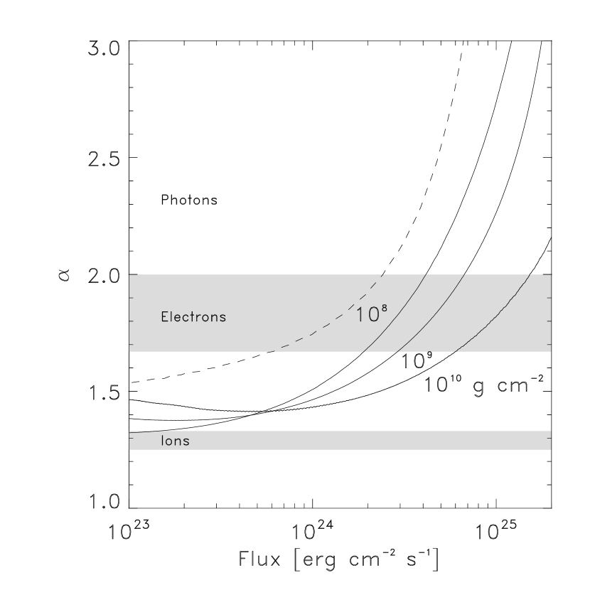
Figure 6: The light curve slope as a function of flux as calculated in multizone models of a cooling layer (solid curves) with column depths $y=10^{8}$, $10^{9}$, and $10^{10}\ {\rm g\ cm^{-2}}$. For comparison we show the one-zone model result for $y=10^{8}\ {\rm g\ cm^{-2}}$ as the dashed curve. The gray areas show the expected range of values of $\alpha$ when ions dominate the heat capacity or when electrons dominate the heat capacity, taking the cooling to lie between $L\propto T^{4}$ and $L\propto T^{5}$.

The dependence of the cooling luminosity on the layer temperature depends on the details of the temperature profile in the layer, connecting the temperature near the base of the layer to the temperature at the photosphere. For a constant flux, this relation is determined by integrating the radiative diffusion equation

$$F = -{4acT^{3}\over 3\kappa\rho}{dT\over dr}$$ (9)

where $\kappa$ is the opacity. For constant opacity, the integration gives $F\propto T^{4}$, but the scaling with temperature can be different when the opacity is temperature and depth dependent. For example, the relation between surface temperature $T_{\rm eff}$ and the temperature deep in the crust at densities of $\rho\gtrsim 10^{10}\ {\rm g\ cm^{-3}}$ is $T_{\rm eff}\propto T^{2.2}$ (Gudmundsson et al. 1982). We calculated a series of constant flux temperature profiles in the neutron star envelope to determine the scaling of luminosity with temperature at the base of the layer, $L\propto T^{\gamma}$. We find that for column depths typical of X-ray burst ignition, $10^{8}$–$10^{9}\ {\rm g\ cm^{-2}}$, $\gamma\approx 4$–$5$.

Following through the argument leading to Eq. 4 for $L\propto T^{\gamma}$ gives $\alpha=\gamma/(\gamma-1-\beta)$. Therefore for the range $\gamma=4$–$5$, we expect $\alpha=1.25$–$1.33$ when ions dominate the heat capacity ($\beta=0$), $\alpha=1.67$–$2.0$ when electrons dominate the heat capacity, and larger values of $\alpha$ when radiation makes a significant contribution. These values are shown as gray regions in the histogram of $\alpha$ in Figure 5. We see that there is a good match to the observed values of $\alpha$ when degenerate electrons or radiation is taken into account.

To further investigate the agreement between the predicted and observed values of $\alpha$, we calculated the expected values of $\alpha$ as a function of the flux from the star. We did this in two ways. The first is a one-zone model based on the argument leading to Eq. 4. For a given flux $F$ and layer column depth $y$, we first use our constant flux envelope models to find the temperature at the base of the layer. We calculate the heat capacity temperature scaling $\beta$ using the base temperature and base pressure $P=gy$, where $g$ is the gravitational acceleration (where we use the fact that the layer is in hydrostatic balance). To validate the one-zone approach, we also calculated a series of multizone cooling models following Cumming & Macbeth (2004) but extended to shallower layers. In these models, we heated a layer of a given depth by depositing the amount of energy expected from complete helium burning ($1.6\ {\rm MeV}$ per nucleon) and then followed the cooling of the layer by integrating the thermal diffusion equation. We then calculated the local slope of the light curve $\alpha=-d\ln L/d\ln t$ as a function of time and therefore as a function of flux.

The results of the multizone models are shown as solid curves in Fig. 6 for column depths $y=10^{8}$, $10^{9}$, and $10^{10}\ {\rm g\ cm^{-2}}$. The one-zone model results for $y=10^{8}\ {\rm g\ cm^{-2}}$ are shown as the dashed curve. The shape of the one-zone model curve matches the multizone model well, but the one-zone model decay is everywhere steeper than found in the multizone model. The reason for this is that in the multizone model, which follows the temperature profile of the envelope in detail, a significant amount of heat is conducted inwards as the layer cools, so the effective mass of the cooling layer changes. This is not taken into account in the one-zone model which assumes a fixed column depth $y$ and therefore cools faster (larger $\alpha$).

Fig. 6 shows that the expected behavior is that $\alpha$ will decrease with flux (light curve decay becomes shallower). The reason for this is that initially when the layer is hot, radiation pressure is significant, but later the heat capacity becomes dominated by the electrons and ions. At larger column depths, the influence of both radiation pressure and electrons is smaller, and a smaller range of values of $\alpha$ is explored. The decreasing influence of degenerate electrons towards larger ignition depths comes about because only a fraction $k_{\rm B}T/E_{\rm F}$ of the degenerate electrons near the Fermi surface participates in the thermal energy, and $E_{F}$ increases as the layer becomes thicker.

Contrary to the models, we do not detect a change in $\alpha$ in the data, because all data per burst are consistent with a single power law. For bursts for which the fitted data do not cover the upper decade in flux, this is not unexpected. Most of the change in $\alpha$ is in that range. However, around half the bursts do cover that upper range. Thus, the model appears insufficient. It may be that the base temperature is ill constrained due to insufficient knowledge about the total energy liberated. For example, if the energy per nucleon is 0.6 MeV instead of 1.6 MeV as assumed, which is the number for helium burning to carbon instead of iron, $\alpha$ will remain below 2.05 for $y=10^{8}$ g cm^-2 for a flux below 10²⁵ erg cn^-2s^-1. This compares to $\alpha<2.8$ for an energy release of 1.6 MeV per nucleon. Measuring this is difficult for PRE bursts, because a significant fraction of the energy is invisible. This may be a subject of future refined modeling.

The spread of $\alpha$ from burst to burst is in line with the above explanation with degenerate electrons and photons, because one expects a spread in ignition conditions from burst to burst. In principle, $\alpha$ may constrain the ignition conditions. For instance, a high $\alpha$ points to a low ignition depth. We tried to verify a dependence between $\alpha$ and ignition depth, by assuming that burst duration as measured with $\tau$ depends monotonically on ignition depth (see Cumming & Macbeth 2004). Figure 7 shows $\alpha$ versus $\tau$. There is no correlation between both parameters, except that the longest (super) burst has the lowest $\alpha$, which is consistent with $\alpha=4/3$. The absence of correlation for ordinary and intermediate duration bursts is probably due to the fact that $\tau$ is not an accurate enough proxy for ignition depth. More detailed light curve modeling that includes early times in intermediate duration bursts is necessary to make a more accurate verification.

Figure 7: Measurements of $\alpha$ versus $\tau$. Horizontal bars are simple markers (exponential function are bad fits to the data) and vertical bars $1\sigma$ errors of $\alpha$. There is no clear correlation between both parameters, except that the longest burst has the lowest value.

5 Conclusion

We have verified, for a representative set of 35 ordinary thermonuclear X-ray bursts from 14 neutron stars, that the radiative decay follows a power law rather than an exponential decay function, and find that the decay index of the power law is steeper than seen in long superbursts (1.8 versus 1.3). Also, it varies from burst to burst, even if from the same neutron star. We hypothesize that this is due to the influence of degenerate electrons and photons on the heat capacity of the ignited layer.

We are unable to confirm this hypothesis through independent measurements of ignition depths or through detection of a change in $\alpha$. That will only be possible through more complete modeling of burst light curves, particularly at early phases when the cooling wave is traveling from the photosphere to the ignition depth. That is not straightforward, because data from that phase suffer from the effects of photospheric expansion. Therefore, the model will have to include those effects. Currently, there are no such models. If it would become possible to confirm the relationship between ignition depth and $\alpha$ for a number of bursts, measurement of $\alpha$ might yield a valuable constraint on ignition depth.