A conjugate class of random probability measures based on tilting and with its posterior analysis

Abstract

This article constructs a class of random probability measures based on exponentially and polynomially tilting operated on the laws of completely random measures. The class is proved to be conjugate in that it covers both prior and posterior random probability measures in the Bayesian sense. Moreover, the class includes some common and widely used random probability measures, the normalized completely random measures (James (Poisson process partition calculus with applications to exchangeable models and Bayesian nonparametrics (2002) Preprint), Regazzini, Lijoi and Prünster (Ann. Statist. 31 (2003) 560–585), Lijoi, Mena and Prünster (J. Amer. Statist. Assoc. 100 (2005) 1278–1291)) and the Poisson–Dirichlet process (Pitman and Yor (Ann. Probab. 25 (1997) 855–900), Ishwaran and James (J. Amer. Statist. Assoc. 96 (2001) 161–173), Pitman (In Science and Statistics: A Festschrift for Terry Speed (2003) 1–34 IMS)), in a single construction. We describe an augmented version of the Blackwell–MacQueen Pólya urn sampling scheme (Blackwell and MacQueen (Ann. Statist. 1 (1973) 353–355)) that simplifies implementation and provide a simulation study for approximating the probabilities of partition sizes.

1 Introduction

Random probability measures derived from normalized independent increment processes have been studied for decades. Kingman [27] considers normalization over subordinators of Lévy processes with only positive jumps. Regazzini et al. [44] introduce the class of the normalized random measures with independent increments (normalized completely random measures) for studying the probabilistic properties of mean functionals of random probability measures. Investigations for statistical modeling are available in James [18], Lijoi et al. [32] and James et al. [22].

In Bayesian non-parametric statistics, the normalized random process is considered to be an unknown parameter and the posterior distribution of the process is usually of interest. The most popular class of such random processes for statistical modelling is the Dirichlet process (Ferguson [12]; Lo [36]). The Dirichlet process is appealing because it induces model flexibility and it is also conjugate in the sense that the posterior process, the process conditional on the data, is also a Dirichlet process. In fact, a surprising result shown in James et al. [21] states that only the Dirichlet process has the conjugacy property among the random probability measures in the class of normalized independent increment processes. In the present work, we are able to show that it is not the case for a richer class of normalized processes. The class of normalized processes considered in this article is derived based on tilting, in particular, exponentially and polynomially tilting operated on the laws of completely random measures and this yields the class of laws containing the prior random probability measures and their posteriors in the Bayesian sense. So, the random probabilities in this class is conjugate.

Tilting the laws of random processes provides a way to enrich the class of random processes through change of measure. For example, Pitman [41] constructs the Poisson–Kingman process by normalizing a random process that has a tilted law of completely random measures. Other well known special cases are the Poisson–Dirichlet process, whose law is constructed by polynomially tilting the laws of positive $\alpha$-stable processes (Pitman [41]), and the beta-gamma process (James [20]), whose law is obtained by polynomially tilting the laws of gamma processes. However, these studies give less attention to the statistical properties of the tilted processes. Our studies in fact focus on showing conjugate property of the random probability measure derived from tilted laws of the completely random measures and providing the posterior analysis of the class of random probability measures.

Applications of non-parametric models are becoming increasingly common in Bayesian statistics. However, implementing non-parametric models is rarely straightforward and often involves Markov chain Monte Carlo (MCMC) algorithms that might require evaluation of complicated functions. This article provides an augmented form of the sampling algorithm, namely the Blackwell–MacQueen Pólya urn sampling scheme, which avoids the necessity of evaluating those functions for some special cases and which we believe would be beneficial to the use of normalized random measures in statistical applications in future. We provide a simulation study concerned with estimating probabilities of partition sizes, a problem that arises in biological speciation (Lijoi et al. [33]). We show our algorithm yields similar results to three other sampling schemes based on the Blackwell–MacQueen Pólya urn distribution.

The article proceeds as follows. Section 2 describes the construction of a class of random probability measures obtained by tilting the laws of completely random measures. Materials presented here are in compact form; we refer the reader to Daley and Vere-Jones [8] for the complete treatment on these topics (see also Kingman [25, 27, 26]; Kallenberg [23, 24]). Section 3 considers a class of random probability measures constructed through polynomially and exponentially tilting the laws of completely random measures. Section 3 also provides details on the prior and posterior distributions, proves the conjugacy property and describes the augmented Blackwell–MacQueen sampling scheme. Section 4 describes two specific examples of the tilting strategy, tilting the laws of the generalized gamma process and the generalized Dirichlet process is demonstrated. Section 5 presents the simulation study. Section 6 concludes the articles and provides a future research perspective. Proofs of theorems and propositions are included in the Appendix.

In addition, as a referee pointed out that theorems in Section 3 are not entirely new and a version of them has appeared in an unpublished manuscript (James [18]), we would like to acknowledge that the class of random probability measures involving polynomially and exponentially tilting was first studied in the manuscript (James [18], Chapter 5), including a posterior analysis. We will further comments on these aspects and connections in Section 3.

2 Construction of the class of random probability measures

Let the triple $(\Omega,\mathfrak{F},\textsf{P})$ be the basic probability space. Assume $\mathbb{X}$ is a Polish space endowed with a metric $d_{\mathbb{X}}$ generating a Borel $\sigma$-field $\mathcal{B}(\mathbb{X})$. Let $\mathcal{M}_{\mathbb{X}}$ denote the space of boundedly finite measures on $(\mathbb{X},\mathcal{B}(\mathbb{X}))$. A measure is said to be boundedly finite if it is finite on bounded sets. The space $\mathcal{M}_{\mathbb{X}}$ is a Polish space equipped with the metric of weak convergence. This induces the Borel $\sigma$-field $\mathcal{B}(\mathcal{M}_{\mathbb{X}})$. A random measure, $\mu$ say, taking values from $\mathcal{M}_{\mathbb{X}}$, is a measureable mapping $\mu\mathchoice{\nobreak\,\colon}{\nobreak\,\colon}{\nobreak\,\colon\;}{\nobreak\,\colon\;}\Omega\times\mathbb{X}\rightarrow\mathbb{R}^{+}\cup\{0\}$ where $\mathbb{R}^{+}$ denotes the positive real line. For each $\omega\in\Omega$, $\mu(\omega,\cdot)$ is a boundedly finite measure on $(\mathbb{X},\mathcal{B}(\mathbb{X}))$ and $\mu(\omega,A)$ is a random variable for all bounded sets $A\in\mathcal{B}(\mathbb{X})$. For convenience of notation, we write $\mu(A)$ instead of $\mu(\omega,A)$ from now on. For further details, see Daley and Vere-Jones [8], Chapter 9.

A random measure $\mu$ is a completely random measure (crm) on the measure space $(\mathbb{X},\mathcal{B}(\mathbb{X}))$ if for all finite families of pairwise disjoint, bounded Borel sets $A_{1},A_{2},\ldots,A_{k}\in\mathcal{B}(\mathbb{X})$, the random variables $\mu(A_{1})$, $\mu(A_{2}),\ldots,\mu(A_{k})$ are mutually independent. For any crm, there is a representation theorem due to Kingman [25], Theorem 1 (see also Kingman [27] and Kingman [26], Chapter 8), and the theorem is nicely described in Daley and Vere-Jones [8], Theorem 10.1.III. The version in Daley and Vere-Jones [8], Theorem 10.1.III, says that a crm $\mu$ can be represented as a sum of an atomic measure with countably many fixed atoms, a deterministic non-atomic measure and a measure derived from a Poisson process. The representation is given by

$$\mu(A)=\sum_{k=1}^{\infty}U_{k}\delta_{x_{k}}(A)+\lambda(A)+\int_{\mathbb{R}^{+}}yN(A,\mathrm{d}y),\qquad A\in\mathcal{B}(\mathbb{X}),$$ (1)

where the sequence $\{x_{1},x_{2},\ldots\}$ is the countable set of fixed atoms of $\mu$, $\{U_{1},U_{2},\ldots\}$ is a sequence of mutually independent non-negative random variables, $\lambda$ is a fixed non-atomic boundedly finite measure on $\mathbb{X}$, and $N$ is a Poisson process on $\mathbb{X}\times\mathbb{R}^{+}$. This Poisson process $N$ is independent of $\{U_{1},U_{2},\ldots\}$ and has an intensity measure $\nu$ on $\mathbb{X}\times\mathbb{R}^{+}$. The intensity $\nu$ satisfies the following two conditions. For every bounded set $A\in\mathcal{B}(\mathbb{X})$,

$$\int_{\mathbb{R}^{+}}\min\{y,s\}\nu(A,\mathrm{d}y)<\infty,\qquad s\in\mathbb{R}^{+},$$ (2)

and

$$\nu\bigl{(}\{x\},\mathbb{R}^{+}\bigr{)}=0,\qquad x\in\mathbb{X}.$$ (3)

Notice that conditions (2) and (3) guarantee that the random measure $\int_{\mathbb{R}^{+}}yN(\cdot,\mathrm{d}y)$ is boundedly finite on $\mathbb{X}$ and has no fixed atoms respectively (see also Kallenberg [24], Chapter 12).

The Poisson process in (1) can be considered as a marked Poisson process on $\mathbb{X}$ having mark space $\mathbb{R}^{+}$. Again the product space $\mathbb{X}\times\mathbb{R}^{+}$ is a Polish space with a suitable metric $d_{\mathbb{X}\times\mathbb{R}^{+}}$ extended from $d_{\mathbb{X}}$. The Borel $\sigma$-field of the Polish space $\mathbb{X}\times\mathbb{R}^{+}$ is given by $\mathcal{B}(\mathbb{X}\times\mathbb{R}^{+})=\mathcal{B}(\mathbb{X})\otimes\mathcal{B}(\mathbb{R}^{+})$ where $\mathcal{B}(\mathbb{R}^{+})$ denotes the $\sigma$-field generated by the open subsets of $\mathbb{R}^{+}$. Then the Poisson process $N$ is a mapping $N\mathchoice{\nobreak\,\colon}{\nobreak\,\colon}{\nobreak\,\colon\;}{\nobreak\,\colon\;}\Omega\times\mathbb{X}\times\mathbb{R}^{+}\rightarrow\mathbb{Z}^{+}\cup\{0\}$ where $\mathbb{Z}^{+}$ denotes the positive integers. This Poisson process takes value from the space of boundedly finite measures $(\mathcal{M}_{\mathbb{X}\times\mathbb{R}^{+}},\mathcal{B}(\mathcal{M}_{\mathbb{X}\times\mathbb{R}^{+}}))$ defined analogous to the space $(\mathcal{M}_{\mathbb{X}},\mathcal{B}(\mathcal{M}_{\mathbb{X}}))$ discussed in the first paragraph. Here we write $N(A,B)$ to represent $N(\omega,A,B)$ for convenience of notation. The intensity measure $\nu$ of this Poisson process is a non-atomic $\sigma$-finite measure $\nu\mathchoice{\nobreak\,\colon}{\nobreak\,\colon}{\nobreak\,\colon\;}{\nobreak\,\colon\;}\mathbb{X}\times\mathbb{R}^{+}\rightarrow\mathbb{R}^{+}\cup\{0\}$. The intensity measure is particularly important since it is the only parameter of the random measure and also the first moment of the measure. It determines the nature of the process and further it also determines the nature of the random measures derived from the Poisson process. Here (3) also implies that $N(\cdot,\mathbb{R}^{+})$ is a simple point process on $\mathbb{X}$. This point process $N(\cdot,\mathbb{R}^{+})$ is called ground process in Daley and Vere-Jones [8], Chapter 9.

Initially, we restrict our attention to the crm on $\mathbb{X}$ without the first two components, the atomic component and the drift, in (1), that is the crm is in the form of

$$\widetilde{\mu}(A):=\int_{\mathbb{R}^{+}}yN(A,\mathrm{d}y),\qquad A\in\mathcal{B}(\mathbb{X}),$$ (4)

with respect to the Poisson process $N$ defined on $\mathbb{X}\times\mathbb{R}^{+}$ with intensity measure $\nu$ satisfying conditions (2) and (3). The law of the crm $\widetilde{\mu}$, denoted by $\mathcal{P}_{\widetilde{\mu}}$, which is derived from the law of the Poisson process. For the sake of simplicity, we say $\widetilde{\mu}$ has the parameter measure $\nu$. The measure $\nu$ can be decomposed into two measures, $\rho_{x}$ and $\eta$, written as $\nu(\mathrm{d}x,\mathrm{d}s)=\eta(\mathrm{d}x)\rho_{x}(\mathrm{d}s)$. Such a decomposition is guaranteed by Kallenberg [23], Appendix 15.3.3, in which the measure $\rho_{x}$ is uniquely determined outside any set of $\nu$ measure zero. Here $\rho_{x}$ is a mapping $\rho_{x}\mathchoice{\nobreak\,\colon}{\nobreak\,\colon}{\nobreak\,\colon\;}{\nobreak\,\colon\;}\mathbb{R}^{+}\rightarrow\mathbb{R}^{+}\cup\{0\}$ for any $x\in\mathbb{X}$ such that $\rho_{x}(A)$ is $\mathbb{X}$ measureable for every bounded set $A\in\mathcal{B}(\mathbb{R}^{+})$ and $\rho_{x}$ is a $\sigma$-finite measure. In particular, when $\rho_{x}$ is dependent on $x\in\mathbb{X}$, the crm $\widetilde{\mu}$ is non-homogeneous. Otherwise, when $\rho_{x}$ is not dependent on $x\in\mathbb{X}$, the crm $\widetilde{\mu}$ is homogeneous. The $\sigma$-finiteness of $\rho_{x}$ ensures the crm $\widetilde{\mu}$ has countably infinite jumps on any bounded set in $\mathcal{B}(\mathbb{X})$. Here $\eta$ is a finite non-atomic measure $\eta\mathchoice{\nobreak\,\colon}{\nobreak\,\colon}{\nobreak\,\colon\;}{\nobreak\,\colon\;}\mathbb{X}\rightarrow\mathbb{R}^{+}\cup\{0\}$. Without loss of generality, the measure $\eta$ is restricted to be a proper probability measure on $\mathbb{X}$. This implies that the total mass of the measure $\widetilde{\mu}$ is finite almost surely. Then a random probability measure could be defined according to the ratio of $\widetilde{\mu}(A)$ and the total mass $\widetilde{\mu}(\mathbb{X})$, that is $\widetilde{G}(A):=\widetilde{\mu}(A)/\widetilde{\mu}(\mathbb{X})$ for $A\in\mathcal{B}(\mathbb{X})$.

Let $h$ be a positive Borel measurable function $h\mathchoice{\nobreak\,\colon}{\nobreak\,\colon}{\nobreak\,\colon\;}{\nobreak\,\colon\;}\mathbb{R}^{+}\cup\{0\}\rightarrow\mathbb{R}^{+}$. Here $h(\widetilde{\mu}(\mathbb{X}))$ is a tilting factor transforming the total mass to a positive scalar. The law of the tilted completely random measure (tilted crm) is given by scaling the law of the crm by the tilting factor. To ensure that the law of the tilted crm is proper, the proportional constant of the law, $E[h(\widetilde{\mu}(\mathbb{X}))]$, is required to be finite, that is,

$$E\bigl{[}h\bigl{(}\widetilde{\mu}(\mathbb{X})\bigr{)}\bigr{]}<\infty.$$ (5)

Definition 2.1.

Let $\widetilde{\mu}$ be a crm defined on $(\mathbb{X},\mathcal{B}(\mathbb{X}))$ in (4). The crm $\widetilde{\mu}$ has a probability measure $\mathcal{P}_{\widetilde{\mu}}$ on $(\mathcal{M}_{\mathbb{X}},\mathcal{B}(\mathcal{M}_{\mathbb{X}}))$ and with the parameter measure $\nu$ that satisfies conditions (2) and (3). Let $h$ be a positive Borel measurable function on the non-negative real line, that satisfies condition (5). A tilted crm, $\widetilde{\mu}_{t}$, defined on $(\mathbb{X},\mathcal{B}(\mathbb{X}))$, has a probability measure $\mathcal{P}_{\widetilde{\mu}_{t}}$ on $(\mathcal{M}_{\mathbb{X}},\mathcal{B}(\mathcal{M}_{\mathbb{X}}))$ such that

$$\mathcal{P}_{\widetilde{\mu}_{t}}(A):=\frac{1}{E[h(\widetilde{\mu}(\mathbb{X}))]}\int_{A}h\bigl{(}\mu(\mathbb{X})\bigr{)}\mathcal{P}_{\widetilde{\mu}}(\mathrm{d}\mu),\qquad A\in\mathcal{B}(\mathcal{M}_{\mathbb{X}}),$$ (6)

with the parameter measures $\nu$ and $h$.

Definition 2.2.

Let $\widetilde{\mu}_{t}$ be a tilted crm with the parameter measures $\nu$ and $h$ defined from Definition 2.1, a normalized tilted crm $\widetilde{G}_{t}$ is given by

$$\widetilde{G}_{t}(A)=\widetilde{\mu}_{t}(A)/\widetilde{\mu}_{t}(\mathbb{X}),\qquad A\in\mathcal{B}(\mathbb{X}),$$ (7)

on $(\mathbb{X},\mathcal{B}(\mathbb{X}))$. This normalized tilted crm $\widetilde{G}_{t}$ is with the parameter measures $\nu$ and $h$.

Notice that when the function is a finite constant ($h(x)=\mathrm{constant}<\infty$), the normalized tilted crm $\widetilde{G}_{t}$ is simply a normalized crm, which has been extensively studied by James [18] and James et al. [22]. Some special cases with various choices of function $h$ and crms have been considered. James [20] considers polynomially tilting the law of gamma process with $h(\mu(\mathbb{X}))=\mu(\mathbb{X})^{-q}$. Pitman [41, 42] constructs the Poisson–Dirichlet process from polynomially tilting the law of positive stable process. These are all interesting special cases covered by the class of the normalized tilted crms which will be further discussed in Section 3.

The total mass is a key ingredient of both normalized crms and normalized tilted crms. We consider the connection between these two total masses and the general framework on a characterization of the masses through the Laplace transform. Let the total masses of crm and tilted crm be $\widetilde{T}:=\widetilde{\mu}(\mathbb{X})$ and $\widetilde{T}_{t}:=\widetilde{\mu}_{t}(\mathbb{X})$. Both $\widetilde{\mu}$ and $\widetilde{\mu}_{t}$ are the mappings to the positive line so that $\widetilde{T}>0$ and $\widetilde{T}_{t}>0$ and the laws of $\widetilde{T}$ and $\widetilde{T}_{t}$ are both absolutely continuous with respect to Lebesgue measure. Their densities, $f_{\widetilde{T}}(y)$ and $f_{\widetilde{T}_{t}}(y)$, are related through the equality

$$f_{\widetilde{T}_{t}}(y)=\frac{h(y)f_{\widetilde{T}}(y)}{\int_{\mathbb{R}^{+}}h(y)f_{\widetilde{T}}(y)\,\mathrm{d}y}.$$ (8)

The Laplace transform of the random variable $\widetilde{T}$ is given by

$$E\bigl{[}\mathrm{e}^{-\lambda\widetilde{T}}\bigr{]}=\int_{\mathbb{R}^{+}}\mathrm{e}^{-\lambda y}f_{\widetilde{T}}(y)\,\mathrm{d}y=\mathrm{e}^{-\psi_{0}(\lambda)},$$

where in general $\psi_{a}(b)$ is given by

$$\psi_{a}(b)=\int_{\mathbb{R}^{+}\times\mathbb{X}}\bigl{(}1-\mathrm{e}^{-bs}\bigr{)}\mathrm{e}^{-as}\rho_{x}(\mathrm{d}s)\eta(\mathrm{d}x),\qquad a\geq 0,b>0.$$ (9)

In terms of the density of $\widetilde{T}$, the Laplace transform of the random variable $\widetilde{T}_{t}$ could be seen as

$$E\bigl{[}\mathrm{e}^{-\lambda\widetilde{T}_{t}}\bigr{]}=\int_{\mathbb{R}^{+}}\mathrm{e}^{-\lambda y}f_{\widetilde{T}_{t}}(y)\,\mathrm{d}y=\int_{\mathbb{R}^{+}}\mathrm{e}^{-\lambda y}\frac{h(y)f_{\widetilde{T}}(y)}{\int_{\mathbb{R}^{+}}h(s)f_{\widetilde{T}}(s)\,\mathrm{d}s}\,\mathrm{d}y.$$ (10)

From (10), it requires to specify $h$ to derive an explicit form. In fact, it is clear that the total masses are connected through the equality (8) and this could be utilized to derive the distributional results of the masses. A further extension on characterizing the random measures may concern the Laplace transform of their functionals, specifically linear functionals, that play an important role in the studies of random measures. One could see it as a generalization from measuring a set (e.g., equation (4)) as an indicator function to measuring a class of functions. Let $BM^{+}(\mathbb{X})$ denote the class of positive Borel measurable functions mapping from $\mathbb{X}$ to $\mathbb{R}^{+}\cup\{0\}$ and all functions in this class vanish outside the bounded sets of $\mathbb{X}$. Let $g$ be a function in $BM^{+}(\mathbb{X})$ and let the functional defined as $\widetilde{\mu}(g):=\int_{\mathbb{X}}g(x)\widetilde{\mu}(\mathrm{d}x)$. This functional is also regarded as a Poisson functional since it has an expression with respect to the Poisson process on $\mathbb{X}\times\mathbb{R}^{+}$, that is $\widetilde{\mu}(g)=\int_{\mathbb{R}^{+}\times\mathbb{X}}g(x)yN(\mathrm{d}x,\mathrm{d}y)$. Then the properties of the crm $\widetilde{\mu}$ could be derived from the Poisson process $N$. For general discussion of functionals and Laplace functionals, see Daley and Vere-Jones [8], Chapters 9, 10. An early application to Bayesian non-parametric statistics would be found in [39] (see also Dykstra and Laud [11]).

3 The normalized random measure derived from the polynomially and exponentially tilted law

Here we aim at showing the conjugacy property of the normalized tilted crm $\widetilde{G}_{t}$ with a specific choice of $h$ (Definition 2.2). First, we take $h$ as follows

$$h(x)=h^{\prime}(x)x^{-q},\qquad q\geq 0,$$ (11)

where $h^{\prime}$ is a positive measurable function $h^{\prime}\mathchoice{\nobreak\,\colon}{\nobreak\,\colon}{\nobreak\,\colon\;}{\nobreak\,\colon\;}\mathbb{R}^{+}\cup\{0\}\rightarrow\mathbb{R}^{+}$ and satisfying condition (5), that is $E[h^{\prime}(\widetilde{\mu}(\mathbb{X}))\widetilde{\mu}(\mathbb{X})^{-q}]<\infty$, but it is not depending on the scalar $q$. Take the normalized tilted crm $\widetilde{G}_{t}$ be a prior random probability measure in the Bayesian non-parametric content, we can show that the posterior of $\widetilde{G}_{t}$ is belong to the same class of random probability measure (Definition 2.2). So the conjugacy property of $\widetilde{G}_{t}$ with the choice of $h$ (11) is immediately revealed. We then consider the polynomially and exponentially tilted law of the crm $\widetilde{\mu}_{t}$, specifically, we take

$$h^{\prime}(x)=\mathrm{e}^{-\gamma x},\qquad\gamma\geq 0,$$ (12)

in (11). This choice covers a rich class of random probability measures and the interest in this choice is desirable. The posterior analysis of this class of tilted crms is given after the conjugacy property has been shown.

In general, the law of the tilted crm $\widetilde{\mu}_{t}$ is given by

$$\mathcal{P}_{\widetilde{\mu}_{t}}(A)=\frac{1}{E[h^{\prime}(\widetilde{\mu}(\mathbb{X}))\widetilde{\mu}(\mathbb{X})^{-q}]}\int_{A}h^{\prime}\bigl{(}\mu(\mathbb{X})\bigr{)}\mu(\mathbb{X})^{-q}\mathcal{P}_{\widetilde{\mu}}(\mathrm{d}\mu),\qquad A\in\mathcal{B}(\mathcal{M}_{\mathbb{X}}).$$

The parameters of both the tilted crm $\widetilde{\mu}_{t}$ and normalized tilted crm $\widetilde{G}_{t}$ are now $q\geq 0$, $h^{\prime}$ and the intensity measure $\nu$ only. In particular, if $h^{\prime}$ is chosen to be $\mathrm{e}^{-\gamma x}$ in (11), the parameters are then $q\geq 0$, $\gamma\geq 0$ and the intensity measure $\nu$. The random probability measures in the class of normalized tilted crms are more general than those in the class of the normalized crms (Regazzini et al. [44]; James et al. [22]); one could easily realize that the tilted crm $\widetilde{\mu}_{t}$ (Definition 2.1) is not necessarily a crm and this could be seen as a generalization of the class.

Remark 3.1.

A referee pointed out that here the exponentially tilting, say $h(x)=\mathrm{e}^{-\gamma x}$, is redundant as the exponentially tilting operation on a crm leads to another crm. So taking $h^{\prime}$ as in (12), such that $h(x)=\mathrm{e}^{-\gamma x}x^{-q}$, operated with a crm is equivalent to taking $h^{\prime}$ as a fixed finite constant, such that $h(x)=x^{-q}$, operated with another crm.

Remark 3.2.

Scaling operation on the law of Poisson random measures and crms has been studied in James [18]. James [18], equation 70, has the same construction as in this work by taking $h^{\prime}$ to be a fixed finite constant in (11), or to be (12) from Definition 2.1.

3.1 The posterior law and structural conjugacy

Consider a sequence of exchangeable random elements taking values in $\mathbb{X}$. These random variables are assumed to be conditionally independent and identically distributed given the normalized tilted crm $\widetilde{G}_{t}$ (Definition 2.2) such that for every integer $n\geq 1$

$$\mathbb{P}(X_{1}\in B_{1},\ldots,X_{n}\in B_{n}|\widetilde{G}_{t})=\prod_{i=1}^{n}\widetilde{G}_{t}(B_{i})=\prod_{i=1}^{n}\frac{\widetilde{\mu}_{t}(B_{i})}{\widetilde{\mu}_{t}(\mathbb{X})},\qquad B_{1},\ldots,B_{n}\in\mathcal{B}(\mathbb{X}),\quad$$ (13)

where $\widetilde{G}_{t}$, or equivalently $\widetilde{\mu}_{t}$, is regarded as a parameter. Then, (13) is the “likelihood” with the parameter $\widetilde{\mu}_{t}$. Let $\mathcal{P}_{\widetilde{\mu}_{t}}^{(\mathbf{X}_{n})}$ indicate the posterior distribution of $\widetilde{\mu}_{t}$, namely the distribution of $\widetilde{\mu}_{t}$ conditional on $\mathbf{X}_{n}$, that is

$$\mathcal{P}_{\widetilde{\mu}_{t}}^{(\mathbf{X}_{n})}(A):=\frac{\mathcal{P}_{\widetilde{\mu}_{t},\mathbf{X}_{n}}(A,B_{1},\ldots,B_{n})}{\mathcal{P}_{\widetilde{\mu}_{t},\mathbf{X}_{n}}(\mathcal{M}_{\mathbb{X}},B_{1},\ldots,B_{n})},\qquad A\in\mathcal{B}(\mathcal{M}_{\mathbb{X}}),B_{1},\ldots,B_{n}\in\mathcal{B}(\mathbb{X}),$$

where $\mathcal{P}_{\widetilde{\mu}_{t},\mathbf{X}_{n}}$ represents the joint distribution of $(\widetilde{\mu}_{t},\mathbf{X}_{n})$ such that

$$\mathcal{P}_{\widetilde{\mu}_{t},\mathbf{X}_{n}}(A,B_{1},\ldots,B_{n})=\int_{A}\prod_{i=1}^{n}\frac{\mu(B_{i})}{\mu(\mathbb{X})}\mathcal{P}_{\widetilde{\mu}_{t}}(\mathrm{d}\mu),\qquad A\in\mathcal{B}(\mathcal{M}_{\mathbb{X}}),B_{1},\ldots,B_{n}\in\mathcal{B}(\mathbb{X}).\qquad$$ (14)

Taking into consideration of the above assumption of conditional independence (13), the joint distribution $\mathcal{P}_{\widetilde{\mu}_{t},\mathbf{X}_{n}}$of $(\widetilde{\mu}_{t},\mathbf{X}_{n})$ is defined on the space $(\mathcal{M}_{\mathbb{X}}\times\mathbb{X}^{n},\mathcal{B}(\mathcal{M}_{\mathbb{X}})\otimes\mathcal{B}(\mathbb{X})^{n})$ for $n=1,2,\ldots$ . Now, considering Definition 2.1 of $\mathcal{P}_{\widetilde{\mu}_{t}}$, one obtains

$$\int_{A}\prod_{i=1}^{n}\frac{\mu(B_{i})}{\mu(\mathbb{X})}\mathcal{P}_{\widetilde{\mu}_{t}}(\mathrm{d}\mu)=\frac{1}{E[h^{\prime}(\widetilde{\mu}(\mathbb{X}))\widetilde{\mu}(\mathbb{X})^{-q}]}\int_{A}\frac{h^{\prime}(\mu(\mathbb{X}))}{\mu(\mathbb{X})^{n+q}}\Biggl{(}\prod_{i=1}^{n}\mu(B_{i})\Biggr{)}\mathcal{P}_{\widetilde{\mu}}(\mathrm{d}\mu),\quad$$ (15)

$$\quad A\in\mathcal{B}(\mathcal{M}_{\mathbb{X}}),B_{1},\ldots,B_{n}\in\mathcal{B}(\mathbb{X}).$$

This shows the key element needed for deriving the posterior law of $\widetilde{\mu}_{t}$ is the law of the crm $\mathcal{P}_{\widetilde{\mu}}$ as seen in the right-hand side of (15). The usual technique to derive the posterior of $\widetilde{\mu}_{t}$ requires application of change of measure or disintegration. So, the major task is to apply change of measure updating the law $\mathcal{P}_{\widetilde{\mu}}$ with the information, namely $(\prod_{i=1}^{n}\mu(B_{i}))$, $h^{\prime}({\mu}(\mathbb{X}))$ and $\mu(\mathbb{X})^{-(n+q)}$, to a posterior law, $\mathcal{P}_{\widetilde{\mu}}^{(\mathbf{X}_{n})}$. Dealing with the term $(\prod_{i=1}^{n}\mu(B_{i}))$ could be simply adopted by the standard arguments (James [18, 19, 20]). The next term $h^{\prime}({\mu}(\mathbb{X}))$ should be chosen explicitly to proceed. When $h^{\prime}({\mu}(\mathbb{X}))=\mathrm{e}^{-\gamma{\mu}(\mathbb{X})}$, change of measure only involves the Laplace transform and doesn’t cost much effort. Eventually, dealing with the term $\mu(\mathbb{X})^{-(n+q)}$ could be somehow challenging. James [18] (see also James et al. [22]) introduces an augmentation approach that allows us to proceed further in particular for this polynomial term $\mu(\mathbb{X})^{-(n+q)}$. This leads to the analysis on the posteriors of the normalized tilted crms.

James [18]’s approach makes use of the gamma identity and introduces an augmented variable. We now address the role of the augmented variable. Here the well-known gamma identity is given by

$$\frac{1}{b^{a}}=\frac{1}{\Gamma(a)}\int_{\mathbb{R}^{+}}\mathrm{e}^{-bu}u^{a-1}\,\mathrm{d}u,\qquad a,b\in\mathbb{R}^{+}.$$ (16)

Then take the term $\mu(\mathbb{X})^{-(n+q)}$ in (15) as $b^{-a}$ in (16), term involving $\mu$ becomes tractable, positioned as an exponent. The integral (numerator) appearing in the right-hand side (15) can be rewritten as

$$\int_{A\times\mathbb{R}^{+}}h^{\prime}(y)\biggl{[}\int_{\mathbb{R}^{+}}\frac{u^{n+q-1}\mathrm{e}^{-uy}}{\Gamma(n+q)}\,\mathrm{d}u\biggr{]}\Biggl{(}\prod_{i=1}^{n}\mu(B_{i})\Biggr{)}\mathbb{P}(\widetilde{\mu}\in\mathrm{d}\mu|\widetilde{T}=y)f_{\widetilde{T}}(y)\,\mathrm{d}y,$$

$$\quad A\in\mathcal{B}(\mathcal{M}_{\mathbb{X}}),B_{1},\ldots,B_{n}\in\mathcal{B}(\mathbb{X}).$$

where $\mathbb{P}(\widetilde{\mu}\in d\mu|\widetilde{T}=y)$ denotes the conditional distribution of $\widetilde{\mu}$ given its’ total mass $\widetilde{T}=\widetilde{\mu}(\mathbb{X})$. Rewriting the last expression by replacing $f_{\widetilde{T}}$ with its expression in term $f_{\widetilde{T}_{t}}$ (8), from (15) and (3.1) one finally gets

$$\int_{A}\prod_{i=1}^{n}\frac{\mu(B_{i})}{\mu(\mathbb{X})}\mathcal{P}_{\widetilde{\mu}_{t}}(\mathrm{d}\mu)=\int_{A\times\mathbb{R}^{+}\times\mathbb{R}^{+}}\Biggl{(}\prod_{i=1}^{n}\frac{\mu(B_{i})}{y}\Biggr{)}\mathbb{P}(\widetilde{\mu}\in\mathrm{d}\mu|\widetilde{T}=y)\ell_{n}(y,u)\,\mathrm{d}y\,\mathrm{d}u,\quad$$ (18)

$$\quad A\in\mathcal{B}(\mathcal{M}_{\mathbb{X}}),B_{1},\ldots,B_{n}\in\mathcal{B}(\mathbb{X}).$$

where

$$\ell_{n}(y,u)=\frac{u^{n+q-1}\mathrm{e}^{-uy}y^{n+q}}{\Gamma(n+q)}f_{\widetilde{T}_{t}}(y),\qquad u>0,y>0.$$ (19)

Here $\ell_{n}$ is a joint probability density on $\mathbb{R}^{+}\times\mathbb{R}^{+}$. Without loss of generality, we assume that $(\Omega,\mathfrak{F},\textsf{P})$ is large enough to support a sequence $U_{n}$ of random numbers such that the distribution of $(U_{n},\widetilde{T}_{t})$ admits $\ell_{n}$ as density function. Then, it follows that

$$f_{U_{n}}(u)=\int_{\mathbb{R}^{+}}\ell_{n}(y,u)\,\mathrm{d}y=\frac{u^{n+q-1}}{\Gamma(n+q)}\int_{\mathbb{R}^{+}}y^{n+q}\mathrm{e}^{-uy}f_{\widetilde{T}_{t}}(y)\,\mathrm{d}y,\qquad u>0.$$ (20)

Here $f_{U_{n}}$ is a probability density for $U_{n}$. In view of these elementary developments, one can disintegrate the law of $(\widetilde{\mu}_{t},\mathbf{X}_{n})$ as follows

$$\int_{A}\prod_{i=1}^{n}\frac{\mu(B_{i})}{\mu(\mathbb{X})}\mathcal{P}_{\widetilde{\mu}_{t}}(\mathrm{d}\mu)=\int_{A\times\mathbb{R}^{+}\times\mathbb{R}^{+}}\Biggl{(}\prod_{i=1}^{n}\frac{\mu(B_{i})}{y}\Biggr{)}$$

$$\hskip 141.0pt{}\times\mathbb{P}(\widetilde{\mu}\in\mathrm{d}\mu|\widetilde{T}=y)f_{\widetilde{T}|U_{n}}(y|u)f_{U_{n}}(u)\,\mathrm{d}u\,\mathrm{d}y,\quad$$ (21)

$$\quad A\in\mathcal{B}(\mathcal{M}_{\mathbb{X}}),B_{1},\ldots,B_{n}\in\mathcal{B}(\mathbb{X}),$$

where

$$f_{\widetilde{T}|U_{n}}(y|u)=\frac{\ell_{n}(u,y)}{\int_{\mathbb{R}^{+}}\ell_{n}(u,y)\,\mathrm{d}y}=\frac{y^{n+q}\mathrm{e}^{-uy}}{E[\widetilde{T}_{t}^{n+q}\mathrm{e}^{-u\widetilde{T}_{t}}]}f_{\widetilde{T}_{t}}(y),\qquad y>0.$$

This disintegration (3.1) shows the role of $U_{n}$ as an augmented variable.

Remark 3.3.

The representation of the density (20) suggests that $U_{n}$ has the gamma distribution with a random scale $\widetilde{T}_{t}$ which has the density $f_{\widetilde{T}_{t}}$. Given $\widetilde{T}_{t}$, $U_{n}$ has the gamma distribution with parameters $(n+q,\widetilde{T}_{t})$. The product of the random variables, $U_{n}\widetilde{T}_{t}$, has the gamma distribution with parameters $(n+q,1)$ and independent of $\widetilde{T}_{t}$.

Before proceeding to the posterior distribution, additional notations are introduced. The normalized tilted crm $\widetilde{G}_{t}$ is almost surely discrete. A random sample $\mathbf{X}_{n}$ of $\widetilde{G}_{t}$ usually contains ties. We can always express $\mathbf{X}_{n}$ by two elements, namely a partition and distinct values. Here $\mathbf{p}_{n}$ is a partition of the integers $\{1,\ldots,n\}$ that are the indices of $\mathbf{X}_{n}$ and $\mathbf{Y}_{\aleph(\mathbf{p}_{n})}=\{Y_{1},\ldots,Y_{\aleph(\mathbf{p}_{n})}\}$ represents the distinct values of $\mathbf{X}_{n}$. The partition $\mathbf{p}_{n}$ locates the distinct values from $\mathbf{X}_{n}$ to $\mathbf{Y}_{\aleph(\mathbf{p}_{n})}$ or vice versa. As a result, we have the following equivalent representations

$$\mathbf{X}_{n}=\{X_{1},\ldots,X_{n}\}=\{Y_{1},\ldots,Y_{\aleph(\mathbf{p}_{n})},\mathbf{p}_{n}\}=\{\mathbf{Y}_{\aleph(\mathbf{p}_{n})},\mathbf{p}_{n}\}.$$ (22)

A partition $\mathbf{p}_{n}$ contains $\aleph(\mathbf{p}_{n})$ cells (known as clusters), that is $\mathbf{p}_{n}=\{C_{1},\ldots,C_{\aleph(\mathbf{p}_{n})}\}$. Each cell $C_{k}$ contains the indices of a subset of $\mathbf{X}_{n}$, namely the unique values $Y_{k}$ such that $C_{k}=\{i\mathchoice{\nobreak\,\colon}{\nobreak\,\colon}{\nobreak\,\colon\;}{\nobreak\,\colon\;}X_{i}=Y_{k},i=1,\ldots,n\}$ for $k=1,\ldots,\aleph(\mathbf{p}_{n})$. The number of elements in the cell $k$, $C_{k}$, of the partition is indicated by $n_{k}$, for $k=1,\ldots,\aleph(\mathbf{p}_{n})$, so that $\sum_{k=1}^{\aleph(\mathbf{p}_{n})}n_{k}=n$. Therefore, the union of all cells is the set of all $n$ integers, $\bigcup_{k=1}^{\aleph(\mathbf{p}_{n})}C_{k}=\{1,\ldots,n\}$ and all cells are pairwise mutually exclusive, that is $C_{k}\cap C_{k^{\prime}}=\varnothing$ where $k\neq k^{\prime}$ for $k,k^{\prime}=1,\ldots,\aleph(\mathbf{p}_{n})$. This partition representation is commonly used in Bayesian non-parametric literature (see Lo [36]; Lo and Weng [39]; James [18, 19, 20]) since it well describes the variates generated from those random probability measures and is also useful in expressing the marginal distribution of $\mathbf{X}_{n}$.

Lijoi and Prünster [35] describe the concept of structural conjugacy. A random probability measure, say $G$, is a structurally conjugate random probability measure if the resulting posterior law of $G$ given $\mathbf{X}_{n}=\{X_{1},\ldots,X_{n}\}$, has the same structure. Neutral to the right process (Doksum [10]) is one of the classes that has this property. In the present work, we show that the normalized tilted crms in Definition 2.1 are also structurally conjugate. Here we follow James et al. [22], write $\widetilde{G}_{t}^{(\mathbf{X}_{n})}$ as the posterior normalized tilted crm. Theorem 3.1 shows that the normalized tilted crms in Definition 2.2 have the conjugate property, that is, both $\widetilde{G}_{t}$ and $\widetilde{G}_{t}^{(\mathbf{X}_{n})}$ are in the same class.

Theorem 3.1.

Let $\widetilde{G}_{t}=\widetilde{\mu}_{t}/\widetilde{\mu}_{t}(\mathbb{X})$ be a normalized tilted crm (Definition 2.2) defined on $\mathbb{X}$ with $h$ as in (11), that is $h(x)=h^{\prime}(x)x^{-q}$. The parameters of this normalized tilted crm are given by the Borel measurable function $h^{\prime}$, the measure $\nu$, and the scalar $q\geq 0$. With the prior measure $\widetilde{G}_{t}$ and the likelihood (13), the posterior measure, namely $\widetilde{G}_{t}^{(\mathbf{X}_{n})}$, has the same distribution of a normalized tilted crm such that

$$\widetilde{G}_{t}^{(\mathbf{X}_{n})}\stackrel{{\scriptstyle d}}{{=}}\widetilde{\mu}_{t}^{(\mathbf{X}_{n})}/\widetilde{\mu}_{t}^{(\mathbf{X}_{n})}(\mathbb{X}),$$ (23)

where

1. $\widetilde{\mu}_{t}^{(\mathbf{X}_{n})}$ has the law

   $$\mathcal{P}_{\widetilde{\mu}_{t}}^{(\mathbf{X}_{n})}(A)=\frac{1}{E[h^{\prime}(\widetilde{\mu}^{(\mathbf{X}_{n})}(\mathbb{X}))\widetilde{\mu}^{(\mathbf{X}_{n})}(\mathbb{X})^{-(n+q)}]}\int_{A}h^{\prime}\bigl{(}\mu(\mathbb{X})\bigr{)}\mu(\mathbb{X})^{-(n+q)}\mathcal{P}_{\widetilde{\mu}}^{(\mathbf{X}_{n})}(\mathrm{d}\mu)$$

   for $A\in\mathcal{B}(\mathcal{M}_{\mathbb{X}})$.

2. $\widetilde{\mu}^{(\mathbf{X}_{n})}$ is a normalized tilted crm whose law $\mathcal{P}_{\widetilde{\mu}}^{(\mathbf{X}_{n})}$, has the same law as

   $$\widetilde{\mu}+\sum_{k=1}^{\aleph(\mathbf{p}_{n})}J_{k}^{(\mathbf{X}_{n})}\delta_{Y_{k}},$$ (24)

   where $\delta_{a}$ is the Dirac delta function evaluated at $a$, $\widetilde{\mu}$ is a crm with law $\mathcal{P}_{\widetilde{\mu}}$ and intensity measure $\nu$, $\{Y_{1},\ldots,Y_{\aleph(\mathbf{p}_{n})}\}$ is a sequence of fixed points of discontinuity, and $\{J_{1}^{(\mathbf{X}_{n})},\ldots,J_{\aleph(\mathbf{p}_{n})}^{(\mathbf{X}_{n})}\}$ are the corresponding jumps.

3. Conditional on $\mathbf{X}_{n}$, each jump $J_{k}^{(\mathbf{X}_{n})}$ has the conditional distribution

   $$\mathbb{P}\bigl{(}J_{k}^{(\mathbf{X}_{n})}\in\mathrm{d}s\bigr{)}=\frac{s^{n_{k}}\rho_{Y_{k}}(\mathrm{d}s)}{\int_{\mathbb{R}^{+}}s^{n_{k}}\rho_{Y_{k}}(\mathrm{d}s)},\qquad k=1,\ldots,\aleph(\mathbf{p}_{n}).$$

4. Conditional on $\mathbf{X}_{n}$, $\widetilde{\mu}$ and $\{J_{1}^{(\mathbf{X}_{n})},\ldots,J_{\aleph(\mathbf{p}_{n})}^{(\mathbf{X}_{n})}\}$ are independent.

Proof.

See Appendix .1. ∎

In Theorem 3.1, the posterior law of $\widetilde{\mu}_{t}$, namely $\widetilde{\mu}_{t}^{(\mathbf{X}_{n})}$, is shown to have the tilted law of the crm $\widetilde{\mu}^{(\mathbf{X}_{n})}$, which has the law $\mathcal{P}_{\widetilde{\mu}}^{(\mathbf{X}_{n})}$, where the tilting factor is updated to $h^{\prime}(\widetilde{\mu}^{(\mathbf{X}_{n})}(\mathbb{X}))\widetilde{\mu}^{(\mathbf{X}_{n})}(\mathbb{X})^{-(n+q)}$. Under the normalization of the process, the posterior of the random probability measure becomes $\widetilde{G}_{t}^{(\mathbf{X}_{n})}\stackrel{{\scriptstyle d}}{{=}}\widetilde{\mu}_{t}^{(\mathbf{X}_{n})}/\widetilde{\mu}_{t}^{(\mathbf{X}_{n})}(\mathbb{X})$. This confirms the conjugate property of the normalized tilted crm.

Remark 3.4.

Following Remark 3.2, the posterior distribution discussed in James [18], Chapter 5, over the scaling operation on crms has been established in James [18], Corollary 5.1. This result is a version of Theorem 3.1. Furthermore, James [18], Theorem 5.1, also supplies the posterior law of the corresponding Poisson random measure. In particular, putting statements i and ii of James [18], Corollary 5.1, and statements i and ii of James [18], Proposition 5.2, together is equivalent to Theorem 3.1.

A special case of the tilted crm (Definition 2.1) that takes $h(x)=\mathrm{e}^{-\gamma x}x^{-q}$ is of interest. The following theorem, Theorem 3.2, describes an augmented posterior law of $\widetilde{G}_{t}$ and $\widetilde{\mu}_{t}$, denoted by $\widetilde{G}_{t}^{(U_{n},\mathbf{X}_{n})}$ and $\widetilde{\mu}_{t}^{(U_{n},\mathbf{X}_{n})}$, that are the conditional laws of $\widetilde{G}_{t}$ and $\widetilde{\mu}_{t}$, respectively, given both $U_{n}$ and $\mathbf{X}_{n}$.

Theorem 3.2.

Let $\widetilde{G}_{t}=\widetilde{\mu}_{t}/\widetilde{\mu}_{t}(\mathbb{X})$ be a normalized tilted crm (Definition 2.2) on $\mathbb{X}$ with $h$ as in (11) and $h^{\prime}$ as in (12), that is $h(x)=\mathrm{e}^{-\gamma x}x^{-q}$. The parameters of this normalized tilted crm are given by the measure $\nu$, and the scalers $q\geq 0$ and $\gamma\geq 0$. With the prior measure $\widetilde{G}_{t}$ and the likelihood (13), the conditional posterior measure, namely $\widetilde{G}_{t}^{(U_{n},\mathbf{X}_{n})}$, given $U_{n}$ and $\mathbf{X}_{n}=\{X_{1},\ldots,X_{n}\}$ has the same distribution of a normalized crm such that

$$\widetilde{G}_{t}^{(U_{n},\mathbf{X}_{n})}\stackrel{{\scriptstyle d}}{{=}}\widetilde{\mu}^{(U_{n},\mathbf{X}_{n})}/\widetilde{\mu}^{(U_{n},\mathbf{X}_{n})}(\mathbb{X}),$$

where

1. $\widetilde{\mu}^{(U_{n},\mathbf{X}_{n})}$ is a crm with the same law as

   $$\widetilde{\mu}^{(U_{n})}+\sum_{k=1}^{\aleph(\mathbf{p}_{n})}J_{k}^{(U_{n},\mathbf{X}_{n})}\delta_{Y_{k}},$$ (25)

   where $\widetilde{\mu}^{(U_{n})}$ is a crm with intensity $\nu(\mathrm{d}x,\mathrm{d}s)=\eta(\mathrm{d}x)\times\mathrm{e}^{-s(\gamma+U_{n})}\rho_{x}(\mathrm{d}s)$, $\{Y_{1},\ldots,\break Y_{\aleph(\mathbf{p}_{n})}\}$ is a sequence of fixed points of discontinuity, and $\{J_{1}^{(U_{n},\mathbf{X}_{n})},\ldots,J_{\aleph(\mathbf{p}_{n})}^{(U_{n},\mathbf{X}_{n})}\}$ are the corresponding jumps.

2. Conditional on $U_{n}$ and $\mathbf{X}_{n}$, each jump $J_{k}^{(U_{n},\mathbf{X}_{n})}$ has the conditional density

   $$\mathbb{P}\bigl{(}J_{k}^{(U_{n},\mathbf{X}_{n})}\in\mathrm{d}s\bigr{)}=\frac{s^{n_{k}}\mathrm{e}^{-s(\gamma+U_{n})}\rho_{Y_{k}}(\mathrm{d}s)}{\int_{\mathbb{R}^{+}}s^{n_{k}}\mathrm{e}^{-s(\gamma+U_{n})}\rho_{Y_{k}}(\mathrm{d}s)},\qquad k=1,\ldots,\aleph(\mathbf{p}_{n}).$$

3. Conditional on $U_{n}$ and $\mathbf{X}_{n}$, $\mu^{(U_{n})}$ and $\{J_{1}^{(U_{n},\mathbf{X}_{n})},\ldots,J_{\aleph(\mathbf{p}_{n})}^{(U_{n},\mathbf{X}_{n})}\}$ are independent.

4. Conditional on $\mathbf{X}_{n}$, $U_{n}$ has the density

   $$f_{U_{n}|\mathbf{X}_{n}}(u)=\frac{\mathrm{e}^{-\psi_{0}(\gamma+u)}\prod_{k=1}^{\aleph(\mathbf{p}_{n})}\tau_{n_{k},Y_{k}}(\gamma+u)u^{n+q-1}}{\int_{\mathbb{R}^{+}}\mathrm{e}^{-\psi_{0}(\gamma+u)}\prod_{k^{\prime}=1}^{\aleph(\mathbf{p}_{n})}\tau_{n_{k^{\prime}},Y_{k^{\prime}}}(\gamma+u)u^{n+q-1}\,\mathrm{d}u},$$ (26)

   where

   $$\tau_{m,z}(a)=\int_{\mathbb{R}^{+}}s^{m}\mathrm{e}^{-sa}\rho_{z}(\mathrm{d}s),\qquad m>0,z\in\mathbb{X},a\geq 0,$$ (27)

   and $\psi_{a}(b)$ for $a\geq 0$ and $b\geq 0$ is defined in (9).

Proof.

See Appendix .2. ∎

Theorem 3.2 shows that the augmented posterior random probability measure $\widetilde{G}_{t}^{(U_{n},\mathbf{X}_{n})}$ has the same distribution of a normalized crm and further also provides the posterior distribution of the augmented variables $U_{n}$, $f_{U_{n}|\mathbf{X}_{n}}$. Combining these two yields the posterior random probability measure $\widetilde{G}_{t}^{(\mathbf{X}_{n})}$. This is certainly useful in applications of Bayesian non-parametric. For example, this theorem could be useful in simulating the posterior normalized tilted crm $\widetilde{G}_{t}^{(\mathbf{X}_{n})}$ that is desirable in some applications.

Remark 3.5.

The posterior distribution of the tilted crm, namely $\widetilde{\mu}^{(\mathbf{X}_{n})}_{t}$, can be achieved by mixing the law in (25) (Theorem 3.2, statement 1) over the distribution of $U_{n}$ given $\mathbf{X}_{n}$ in (26) (Theorem 3.2, statement 4). This is equivalent to the law of the tilted crm in statement i of James [18], Corollary 5.1.

3.2 Generalized Blackwell and MacQueen Pólya urn sampling scheme and marginal distribution of partitions

Blackwell and MacQueen [3] first introduce the Pólya urn sampling scheme for the Dirichlet process and this scheme can be utilized to generate random sequences from the Dirichlet process. This employs so called the Blackwell–MacQueen Pólya (bmp) urn formula, that is the predictive distribution of the Dirichlet process random sequences. Lo [37] also shows that this bmp urn formula can be used to characterize the Dirichlet process. James et al. [22] generalize the Blackwell–MacQueen Pólya (bmp) urn formula for the normalized crms, namely Generalized Blackwell–MacQueen Pólya (gbmp) urn formula. A further generalization will be considered for the normalized tilted crm in this section.

We consider a normalized tilted crm $\widetilde{G}_{t}$ with $h(x)=\mathrm{e}^{-\gamma x}x^{-q}$ in Definition 2.2. Here the gbmp urn formula for this normalized tilted crm will be presented under two formulations, namely the unconditional and the conditional gbmp urn formulas for the normalized tilted crm. The unconditional gbmp urn formula is simply the predictive distribution, $\mathbb{P}\{X_{n+1}\in\mathrm{d}x|\mathbf{X}_{n}\}$ where $\{X_{n+1},\mathbf{X}_{n}\}$ is the random sequence drawn from the normalized tilted crm $\widetilde{G}_{t}$. The conditional gbmp urn formula is the augmented version of gbmp urn formula derived from Theorem 3.2. An impression directly comes to the mind is that the conditional urn formula, namely $\mathbb{P}\{X_{n+1}\in\mathrm{d}x|\mathbf{X}_{n},U_{n}\}$ could be derived according to the predictive distribution $\mathbb{P}\{X_{n+1}\in\mathrm{d}x|\mathbf{X}_{n}\}=E[\mathbb{P}\{X_{n+1}\in\mathrm{d}x|\mathbf{X}_{n},U_{n}\}|\mathbf{X}_{n}]$ with respect to the distribution $U_{n}$ given $\mathbf{X}_{n}$, $f_{U_{n}|\mathbf{X}_{n}}$ (26). However, the term $\mathbb{P}\{X_{n+1}\in\mathrm{d}x|\mathbf{X}_{n},U_{n}\}$ is not necessarily a proper distribution. A rescaling over both $\mathbb{P}\{X_{n+1}\in\mathrm{d}x|\mathbf{X}_{n},U_{n}\}$ and $f_{U_{n}|\mathbf{X}_{n}}$ with a factor involving terms like $U_{n}$ seems to be needed. This leads to a new variable $\widetilde{U}_{n}$ introduced and this new variable has a tilted density of $U_{n}$. So, we obtain a proper distribution $\mathbb{P}\{X_{n+1}\in\mathrm{d}x|\mathbf{X}_{n},\widetilde{U}_{n}\}$ and also the conditional gbmp urn formula is established by mixing over $\widetilde{U}_{n}$.

Proposition 3.1.

Let $\widetilde{G}_{t}=\widetilde{\mu}_{t}/\widetilde{\mu}_{t}(\mathbb{X})$ be a normalized tilted crm (Definition 2.2) defined on $\mathbb{X}$ with $h$ as in (11) and $h^{\prime}$ as in (12), that is $h(x)=\mathrm{e}^{-\gamma x}x^{-q}$. The parameters of this normalized tilted crm are given by the measure $\nu$, and the scalers $q\geq 0$ and $\gamma\geq 0$. Then,

1. The predictive distribution for $X_{n+1}$ given $\mathbf{X}_{n}=\{X_{1},\ldots,X_{n}\}$ is given by

   $$\mathbb{P}\{X_{n+1}\in\mathrm{d}x|\mathbf{X}_{n}\}=\frac{\omega_{n,\aleph(\mathbf{p}_{n})+1}(x)}{\phi(\mathbf{X}_{n})}\eta(\mathrm{d}x)+\sum_{k=1}^{\aleph(\mathbf{p}_{n})}\frac{\omega_{n,k}(Y_{k})}{\phi(\mathbf{X}_{n})}\delta_{Y_{k}}(\mathrm{d}x),$$ (28)

   where

   $$\phi(\mathbf{X}_{n}) = \int_{\mathbb{X}}\omega_{n,\aleph(\mathbf{p}_{n})+1}(x)\eta(\mathrm{d}x)+\sum_{k=1}^{\aleph(\mathbf{p}_{n})}\omega_{n,k}(Y_{k}),$$

   $$\omega_{n,\aleph(\mathbf{p}_{n})+1}(x) = \int_{\mathbb{R}^{+}}u\tau_{1,x}(\gamma+u)f_{U_{n}|\mathbf{X}_{n}}(u)\,\mathrm{d}u\quad\mbox{and}$$

   $$\omega_{n,k}(Y_{k}) = \int_{\mathbb{R}^{+}}u\frac{\tau_{n_{k}+1,Y_{k}}(\gamma+u)}{\tau_{n_{k},Y_{k}}(\gamma+u)}f_{U_{n}|\mathbf{X}_{n}}(u)\,\mathrm{d}u,\qquad k=1,\ldots,\aleph(\mathbf{p}_{n}).$$

2. Conditional on $\widetilde{U}_{n}$, the predictive distribution for $X_{n+1}$ given $\mathbf{X}_{n}=\{X_{1},\ldots,X_{n}\}$ is given by

   $$\mathbb{P}\{X_{n+1}\in\mathrm{d}x|\mathbf{X}_{n},\widetilde{U}_{n}\}=\frac{\omega_{n,\aleph(\mathbf{p}_{n})+1}(\widetilde{U}_{n},x)}{\phi(\widetilde{U}_{n},\mathbf{X}_{n})}\eta(\mathrm{d}x)+\sum_{k=1}^{\aleph(\mathbf{p}_{n})}\frac{\omega_{n,k}(\widetilde{U}_{n},Y_{k})}{\phi(\widetilde{U}_{n},\mathbf{X}_{n})}\delta_{Y_{k}}(\mathrm{d}x),\qquad$$ (29)

   where

   $$\phi(u,\mathbf{X}_{n}) = \int_{\mathbb{X}}\omega_{n,\aleph(\mathbf{p}_{n})+1}(u,x)\eta(\mathrm{d}x)+\sum_{k=1}^{\aleph(\mathbf{p}_{n})}\omega_{n,k}(u,Y_{k}),$$

   $$\omega_{n,\aleph(\mathbf{p}_{n})+1}(u,x) = u\tau_{1,x}(\gamma+u),$$

   $$\omega_{n,k}(u,Y_{k}) = u\frac{\tau_{n_{k}+1,Y_{k}}(\gamma+u)}{\tau_{n_{k},Y_{k}}(\gamma+u)},\qquad k=1,\ldots,\aleph(\mathbf{p}_{n})\quad\mbox{and}$$

   $$f_{\widetilde{U}_{n}|\mathbf{X}_{n}}(u) = \frac{\phi(u,\mathbf{X}_{n})}{E[\phi(U_{n},\mathbf{X}_{n})|\mathbf{X}_{n}]}f_{U_{n}|\mathbf{X}_{n}}(u),\qquad u>0.$$

3. In addition,

   $$\phi(\mathbf{X}_{n}) = E\bigl{[}\phi(U_{n},\mathbf{X}_{n})|\mathbf{X}_{n}\bigr{]}=n+q,$$

   $$\omega_{n,\aleph(\mathbf{p}_{n})+1}(x) = E\bigl{[}\omega_{n,\aleph(\mathbf{p}_{n})+1}(U_{n},x)|\mathbf{X}_{n}\bigr{]}\quad\mbox{and}$$

   $$\omega_{n,k}(Y_{k}) = E\bigl{[}\omega_{n,k}(U_{n},Y_{k})|\mathbf{X}_{n}\bigr{]},\qquad k=1,\ldots,\aleph(\mathbf{p}_{n}),$$

where $\psi_{a}(b)$ for $a\geq 0$ and $b\geq 0$ defined in (9) and $\tau_{m,z}(a)$ for $m>0$, $z\in\mathbb{X}$ and $a\geq 0$ defined in (27).

Proof.

See Appendix .3. ∎

Proposition 3.1 gives the predictive distribution and the augmented predictive distribution for the sequence $\mathbf{X}_{n}=\{X_{1},\ldots,X_{n}\}$ as in Blackwell and MacQueen [3] and James et al. [22]. Statement 1 of Proposition 3.1 could be viewed as a direct sampling scheme and statement 2 as a conditional sampling scheme that involves iterative sampling with $\widetilde{U}_{n}$ given $\mathbf{X}_{n}$. From statement 1, conditional on $\mathbf{X}_{n}=\{\mathbf{Y}_{\aleph(\mathbf{p}_{n})},\mathbf{p}_{n}\}$, $X_{n+1}$ is sampled from $[\int_{\mathbb{X}}\omega_{n,\aleph(\mathbf{p}_{n})+1}(x)\eta(\mathrm{d}x)]^{-1}\omega_{n,\aleph(\mathbf{p}_{n})+1}(x)\eta(\mathrm{d}x)$ with probability $[\phi(\mathbf{X}_{n})]^{-1}\int_{\mathbb{X}}\omega_{n,\aleph(\mathbf{p}_{n})+1}(x)\*\eta(\mathrm{d}x)$ and the new sample is allocated a new index $\aleph(\mathbf{p}_{n})+1,$ becoming $Y_{\aleph(\mathbf{p}_{n})+1}$. Otherwise $X_{n+1}$ has probability $1-[\phi(\mathbf{X}_{n})]^{-1}\int_{\mathbb{X}}\omega_{n,\aleph(\mathbf{p}_{n})+1}(x)\eta(\mathrm{d}x)$ to be one of the existing sample $\mathbf{Y}_{\aleph(\mathbf{p}_{n})}$. This sequential scheme directly collects sample of size $n$ cumulatively. Statement 2 of Proposition 3.1 suggests an alternative sampling scheme that draws from $\{X_{i},\widetilde{U}_{i}\}$ sequentially for $i=1,\ldots,n$. To initialize the scheme, a sample of $\widetilde{U}_{0}$ from the marginal distribution $f_{\widetilde{U}_{0}}=f_{U_{0}}$ and a sample of $X_{1}$ from $[\int_{\mathbb{X}}\tau_{1,x}(\gamma+\widetilde{U}_{0})\eta(\mathrm{d}x)]^{-1}\tau_{1,x}(\gamma+\widetilde{U}_{0})\eta(\mathrm{d}x)$ are required, then a sample of $\{X_{2},\ldots,X_{n}\}$ can be achieved through iterating the following steps

• Step 1: conditional on $\mathbf{X}_{i}$, sample $\widetilde{U}_{i}$ from $f_{\widetilde{U}_{i}|\mathbf{X}_{i}}$,

• Step 2: conditional on $\mathbf{X}_{i}$ and $\widetilde{U}_{i}$, sample $X_{i+1}$ from $\mathbb{P}\{X_{i+1}\in\mathrm{d}x|\mathbf{X}_{i},\widetilde{U}_{i}\}$,

for $i=1,\ldots,n-1$, where $\mathbf{X}_{i}=\{\mathbf{Y}_{\aleph(\mathbf{p}_{i})},\mathbf{p}_{i}\}$. The scheme described here is more general than those in existing articles and provides alternatives to sample from some common processes, such as the normalized generalized gamma process and the generalized Dirichlet process (see James [18]; Lijoi et al. [31, 32] for a direct sampling scheme). These two cases will be discussed in Section 4.

Remark 3.6.

The joint distribution of $\mathbf{X}_{n}$ can be recovered according to (28) that can be also found in James [18], Theorem 5.2.

Proposition 3.2.

Let $\widetilde{G}_{t}=\widetilde{\mu}_{t}/\widetilde{\mu}_{t}(\mathbb{X})$ be a normalized tilted crm (Definition 2.2) defined on $\mathbb{X}$ with $h$ as in (11) and $h^{\prime}$ as in (12), that is $h(x)=\mathrm{e}^{-\gamma x}x^{-q}$. The parameters of this normalized tilted crm are given by the measure $\nu$, and the scalers $q\geq 0$ and $\gamma\geq 0$. Then,

1. The marginal distribution for $\mathbf{X}_{n}=\{\mathbf{Y}_{\aleph(\mathbf{p}_{n})},\mathbf{p}_{n}\}$ is given by

   $$\frac{\int_{\mathbb{R}^{+}}\mathrm{e}^{-\psi_{0}(\gamma+u)}\prod_{k=1}^{\aleph(\mathbf{p}_{n})}\tau_{n_{k},Y_{k}}(\gamma+u)u^{n+q-1}\,\mathrm{d}u}{\sum_{\mathbf{p}_{n}}\int_{\mathbb{R}^{+}}\mathrm{e}^{-\psi_{0}(\gamma+u)}\prod_{k=1}^{\aleph(\mathbf{p}_{n})}\kappa_{n_{k}}(\gamma+u)u^{n+q-1}\,\mathrm{d}u}\prod_{k=1}^{\aleph(\mathbf{p}_{n})}\eta(\mathrm{d}Y_{k}),$$

   where

   $$\kappa_{m}(a)=\int_{\mathbb{X}}\tau_{m,x}(a)\eta(\mathrm{d}x)=\int_{\mathbb{X}}\biggl{[}\int_{\mathbb{R}^{+}}s^{m}\mathrm{e}^{-sa}\rho_{x}(\mathrm{d}s)\biggr{]}\eta(\mathrm{d}x),\qquad m>0,a\geq 0.$$

2. The marginal distribution for $\mathbf{p}_{n}$ is given by

   $$\frac{\int_{\mathbb{R}^{+}}\mathrm{e}^{-\psi_{0}(\gamma+u)}\prod_{k=1}^{\aleph(\mathbf{p}_{n})}\kappa_{n_{k}}(\gamma+u)u^{n+q-1}\,\mathrm{d}u}{\sum_{\mathbf{p}_{n}}\int_{\mathbb{R}^{+}}\mathrm{e}^{-\psi_{0}(\gamma+u)}\prod_{k=1}^{\aleph(\mathbf{p}_{n})}\kappa_{n_{k}}(\gamma+u)u^{n+q-1}\,\mathrm{d}u}.$$

3. Conditional on $U_{n}$, the distribution for $\mathbf{X}_{n}=\{\mathbf{Y}_{\aleph(\mathbf{p}_{n})},\mathbf{p}_{n}\}$ is given by

   $$\frac{\prod_{k=1}^{\aleph(\mathbf{p}_{n})}\tau_{n_{k},Y_{k}}(\gamma+U_{n})}{\sum_{\mathbf{p}_{n}}\prod_{k=1}^{\aleph(\mathbf{p}_{n})}\kappa_{n_{k}}(\gamma+U_{n})}\prod_{k=1}^{\aleph(\mathbf{p}_{n})}\eta(\mathrm{d}Y_{k}).$$

4. Conditional on $U_{n}$, the distribution for $\mathbf{p}_{n}$ is given by

   $$\frac{\prod_{k=1}^{\aleph(\mathbf{p}_{n})}\kappa_{n_{k}}(\gamma+U_{n})}{\sum_{\mathbf{p}_{n}}\prod_{k=1}^{\aleph(\mathbf{p}_{n})}\kappa_{n_{k}}(\gamma+U_{n})}.$$

5. Conditional on $\mathbf{p}_{n}$, the distribution for $U_{n}$ is given by

   $$\frac{\mathrm{e}^{-\psi_{0}(\gamma+u)}\prod_{k=1}^{\aleph(\mathbf{p}_{n})}\kappa_{n_{k}}(\gamma+u)u^{n+q-1}}{\int_{\mathbb{R}^{+}}\mathrm{e}^{-\psi_{0}(\gamma+u)}\prod_{k=1}^{\aleph(\mathbf{p}_{n})}\kappa_{n_{k}}(\gamma+u)u^{n+q-1}\,\mathrm{d}u},$$

where $\psi_{a}(b)$ for $a\geq 0$ and $b\geq 0$ defined in (9) and $\tau_{m,z}(a)$ for $m>0$, $z\in\mathbb{X}$ and $a\geq 0$ defined in (27).

Proof.

See Appendix .4. ∎

Proposition 3.2 gives the marginal distributions of $\mathbf{X}_{n},$ both conditional and unconditional on $U_{n}$, in statements 1 and 3, respectively. In statements 2 and 4, the proposition gives the distributions of $\mathbf{p}_{n}$ of first $n$ integers $\{1,\ldots,n\}$ both conditional and unconditional on $U_{n}$. The distributions of the partitions are the exchangeable partition probability function (eppf) as they all are symmetric functions of $\{n_{1},\ldots,n_{\aleph(\mathbf{p}_{n})}\}$. A special structure of the eppf, called the Gibbs form, is also available in the conditional case. Specifically, the distribution of the partition, $\mathbf{p}_{n},$ conditional on $U_{n}$ (Statement 4 of Proposition 3.2) has the Gibbs form (Pitman [42], Theorem 4.6, page 86), that is, the eppf is of the form $V_{n,\aleph(\mathbf{p}_{n})}\prod_{k=1}^{\aleph(\mathbf{p}_{n})}W_{n_{k}}$ in which $V_{n,\aleph(\mathbf{p}_{n})}$ is a function of $n$ and $\aleph(\mathbf{p}_{n})$ and $W_{n_{k}}$ is a function of $n_{k}$. Such a partition is called the Gibbs partition and therefore $\mathbf{p}_{n}$ is a Gibbs partition conditional on $U_{n}$ (see Pitman [40] and Pitman [42] for the details of the eppf and the Gibbs form).

Remark 3.7.

The results appear in Proposition 3.2 can be derived from James [18], Theorem 5.2. Some special cases could be found in James [18], Sections 5.3 and 5.4.

4 The tilted version of generalized gamma process and generalized Dirichlet process

We consider the tilted version of two interesting and important classes of measures, namely the generalized gamma process and the generalized Dirichlet process. Tilting these two classes of measures yields the normalized beta-gamma process, the Poisson–Dirichlet process, the normalized generalized gamma process and the Dirichlet process. They all have been extensively studied and have wide applications in both statistics and probability. We now discuss the tilted version of these processes. Let $\widetilde{G}_{t}$ be a normalized tilted crm with $h(x)=\mathrm{e}^{-\gamma x}x^{-q}$ and with $\nu$ chosen in the following subsections.

4.1 Generalized gamma process

The generalized gamma process is considered a building block for random probability measures (James [18]) and has been widely investigated (Lijoi et al. [34]). Earlier studies on this process can be found in modeling survival functions (Hougaard [15]) and in spatial modeling (Wolpert and Ickstadt [45]; Brix [4]). The intensity of the generalized gamma process is given by

$$\nu(\mathrm{d}x,\mathrm{d}s)=\eta(\mathrm{d}x)\times\rho_{x}(\mathrm{d}s)=\eta(\mathrm{d}x)\times\frac{\theta}{\Gamma(1-\alpha)}s^{-1-\alpha}\mathrm{e}^{-b(x)s}\,\mathrm{d}s,$$

$$\quad 0\leq\alpha<1,\theta>0,b(x)\geq 0.$$

This process is an important class since it contains the following well known processes:

1. Taking $0\leq\alpha<1$, $\theta>0$, $b(x)=0$ yields the intensity of positive $\alpha$ stable process,

2. Taking $\alpha=0$, $\theta>0$, $b(x)=b\geq 0$ yields the intensity of gamma process, where $b$ is a known constant,

3. Taking $\alpha=0$, $\theta>0$, $b(x)\geq 0$ yields the intensity of extended gamma process and

4. Taking $\alpha=1/2$, $\theta>0$, $b(x)=b\geq 0$ yields the intensity of inverse Gaussian process, where $b$ is a known constant.

We now consider the normalized random measure derived from the polynomially and exponentially tilted law of the generalized gamma process. An application of Theorem 3.2 and Proposition 3.1 leads to the conditional gbmp urn formula

$$\mathbb{P}\{X_{n+1}\in\mathrm{d}x|\mathbf{X}_{n},\widetilde{U}_{n}\}$$

$$\quad=\biggl{(}{\frac{\theta}{(\gamma+\widetilde{U}_{n}+b(x))^{1-\alpha}}}$$

$$\hphantom{\quad=\biggl{(}}\bigg{/}\biggl{(}{\int_{\mathbb{X}}\frac{\theta}{(\gamma+\widetilde{U}_{n}+b(x))^{1-\alpha}}\eta(\mathrm{d}x)+\sum_{k^{\prime}=1}^{\aleph(\mathbf{p}_{n})}\frac{n_{k^{\prime}}-\alpha}{\gamma+\widetilde{U}_{n}+b(Y_{k^{\prime}})}}\biggr{)}\biggr{)}\eta(\mathrm{d}x)$$ (30)

$$\qquad{}+\sum_{k=1}^{\aleph(\mathbf{p}_{n})}\biggl{(}{\frac{n_{k}-\alpha}{\gamma+\widetilde{U}_{n}+b(Y_{k})}}$$

$$\hphantom{\qquad{}+\sum_{k=1}^{\aleph(\mathbf{p}_{n})}\biggl{(}}\bigg{/}\biggl{(}{\int_{\mathbb{X}}\frac{\theta}{(\gamma+\widetilde{U}_{n}+b(x))^{1-\alpha}}\eta(\mathrm{d}x)+\sum_{k^{\prime}=1}^{\aleph(\mathbf{p}_{n})}\frac{n_{k^{\prime}}-\alpha}{\gamma+\widetilde{U}_{n}+b(Y_{k^{\prime}})}}\biggr{)}\biggr{)}\delta_{Y_{k}}(\mathrm{d}x),$$

and the posterior distribution of $\widetilde{U}_{n}$ is given by

$$f_{\widetilde{U}_{n}|\mathbf{X}_{n}}(u)\propto\cases{\displaystyle\Biggl{[}\int_{\mathbb{X}}\frac{\theta}{(\gamma+u+b(x))^{1-\alpha}}\eta(\mathrm{d}x)+\sum_{k^{\prime}=1}^{\aleph(\mathbf{p}_{n})}\frac{n_{k^{\prime}}-\alpha}{\gamma+u+b(Y_{k^{\prime}})}\Biggr{]}\cr\quad{}\displaystyle\times\frac{\mathrm{e}^{-(\theta/\alpha)\int_{\mathbb{X}}(\gamma+u+b(x))^{\alpha}\eta(\mathrm{d}x)}u^{n+q}}{\prod_{k=1}^{\aleph(\mathbf{p}_{n})}\bigl{(}\gamma+u+b(Y_{k})\bigr{)}^{n_{k}-\alpha}},\qquad 0<\alpha<1,\cr\displaystyle\Biggl{[}\int_{\mathbb{X}}\frac{\theta}{\gamma+u+b(x)}\eta(\mathrm{d}x)+\sum_{k^{\prime}=1}^{\aleph(\mathbf{p}_{n})}\frac{n_{k^{\prime}}}{\gamma+u+b(Y_{k^{\prime}})}\Biggr{]}\cr\quad{}\displaystyle\times\frac{\mathrm{e}^{-\theta\int_{\mathbb{X}}\ln(\gamma+u+b(x))\eta(\mathrm{d}x)}u^{n+q}}{\prod_{k=1}^{\aleph(\mathbf{p}_{n})}\bigl{(}\gamma+u+b(Y_{k})\bigr{)}^{n_{k}}},\hskip 30.0pt\alpha=0.}$$

Notice that when $b(x)=b>0$ and $\alpha=0$, then the condition (5) is reduced to $\theta>q\geq 0$. In fact, when $b(x)=b>0$ and $0<\alpha<1$, then $\theta$ is not required to be greater than $q$ and the condition (5) holds with $q\geq 0$ and $\theta>0$. With a general $b(x)$, the condition (5) is required to be examined. By inspection of (4.1), one could find that when $\alpha=0$ and $b(x)=b$, $X_{n+1}$ is no longer dependent on $\widetilde{U}_{n}$ given the past $\{X_{1},\ldots,X_{n}\}$, that is $\mathbb{P}\{X_{n+1}\in\mathrm{d}x|\mathbf{X}_{n},\widetilde{U}_{n}\}=\mathbb{P}\{X_{n+1}\in\mathrm{d}x|\mathbf{X}_{n}\}$. This fact is also emphasized in Remark 2 of James et al. [22], page 86. This setting with $q=0$ is corresponding to the normalized gamma process or the Dirichlet process and the gbmp urn formula is given by

$$\mathbb{P}\{X_{n+1}\in\mathrm{d}x|\mathbf{X}_{n},\widetilde{U}_{n}\}=\frac{\theta}{\theta+n}\eta(\mathrm{d}x)+\sum_{k=1}^{\aleph(\mathbf{p}_{n})}\frac{n_{k}}{\theta+n}\delta_{Y_{k}}(\mathrm{d}x).$$ (31)

This (31) is the bmp urn formula (see also Blackwell and MacQueen [3]).

Normalized beta-gamma process

The law of the beta-gamma process can be derived from the polynomially tilting the law of the gamma process (James [20]). The beta-gamma process was first introduced for the proof of the Markov–Krein identity of the Dirichlet process mean functionals and since then it has become a useful analytical tool for studying the Dirichlet process (see James [20] and James et al. [22]). Here we mention that Cifarelli and Regazzini [5, 6, 7] were the first works in which this identity was explicitly demonstrated in relation to the research of the law of the Dirichlet process mean functionals. An important fact in James [20] states that a Dirichlet process can be expressed as a normalized beta-gamma process. This becomes an interesting alternative expression of the Dirichlet process that is usually expressed as the normalized gamma process. This expression is given by taking $q>0$, $\gamma=0$, $\alpha=0$, $\theta>q$, $b(x)=b\geq 0$. The condition $\theta>q$ (see also James [20], equation 5, page 649) is equivalent to the condition (5). With $\alpha=0$ and $b(x)=b$, as in the construction through the normalized gamma process, the variable $X_{n+1}$ is not dependent on $\widetilde{U}_{n}$ nor $U_{n}$ given the past $\{X_{1},\ldots,X_{n}\}$.

Poisson–Dirichlet process

The Poisson–Dirichlet process is a common and well known process used in both statistical and probabilistic modeling. This is also called Pitman–Yor process which is coined by Ishwaran and James [16]. This process has been shown to be useful in a variety of interesting applications in combinatorics (Arratia et al. [2]), population genetics (Griffiths and Lessard [14]) and Bayesian statistics (Ishwaran and James [16, 17]). This process was first introduced by Kingman [27] and Pitman and Yor [43] provided a detailed study of its properties. We consider the Poisson–Dirichlet process with parameters ($\alpha,q$) that is equivalent to take $\theta=1$, $\gamma=0$, $b(x)=0$, $q>0$, and $0<\alpha<1$. Special cases include the Dirichlet process and the normalized stable process with parameters ($0,q$) and ($\alpha,0$) respectively. These two processes could be seen as an two parameter extension of the Dirichlet process. Even thought there is an explicit expression of the unconditional gbmp urn formula (Pitman [41, 42]; Ishwaran and James [16, 17]), it is still worth examining the augmented version for the Poisson–Dirichlet process ($\alpha,q$) process. The conditional gbmp urn formula is given by

$$\mathbb{P}\{X_{n+1}\in\mathrm{d}x|\mathbf{X}_{n},\widetilde{U}_{n}\}=\frac{\widetilde{U}_{n}^{\alpha}}{\widetilde{U}_{n}^{\alpha}+n-\alpha\aleph(\mathbf{p}_{n})}\eta(\mathrm{d}x)+\sum_{k=1}^{\aleph(\mathbf{p}_{n})}\frac{n_{k}-\alpha}{\widetilde{U}_{n}^{\alpha}+n-\alpha\aleph(\mathbf{p}_{n})}\delta_{Y_{k}}(\mathrm{d}x),$$

where

$$f_{\widetilde{U}_{n}|\mathbf{X}_{n}}(u) = \frac{q+\alpha\aleph(\mathbf{p}_{n})}{n+q}\frac{\mathrm{e}^{-(1/\alpha)u^{\alpha}}u^{q+\alpha\aleph(\mathbf{p}_{n})+\alpha-1}}{\alpha^{q/\alpha+\aleph(\mathbf{p}_{n})}\Gamma(q/\alpha+\aleph(\mathbf{p}_{n})+1)}$$

$${}+\frac{n-\alpha\aleph(\mathbf{p}_{n})}{n+q}\frac{\mathrm{e}^{-(1/\alpha)u^{\alpha}}u^{q+\alpha\aleph(\mathbf{p}_{n})-1}}{\alpha^{q/\alpha+\aleph(\mathbf{p}_{n})-1}\Gamma(q/\alpha+\aleph(\mathbf{p}_{n}))}.$$

This is equivalent to $\widetilde{U}_{n}\stackrel{{\scriptstyle d}}{{=}}G_{1}^{1/\alpha}$ with probability $(q+\alpha\aleph(\mathbf{p}_{n}))/(n+q)$ and $\widetilde{U}_{n}\stackrel{{\scriptstyle d}}{{=}}G_{2}^{1/\alpha}$ with probability $(n-\alpha\aleph(\mathbf{p}_{n}))/(n+q)$ where $G_{1}$ is a Gamma($q/\alpha+\aleph(\mathbf{p}_{n})+1,1/\alpha$) random variable and $G_{2}$ is a Gamma($q/\alpha+\aleph(\mathbf{p}_{n}),1/\alpha$) random variable.

Normalized generalized gamma process

The normalized generalized gamma process with $\theta>0$, $\gamma=0$, $b(x)=b>0$, $q=0$, and $0<\alpha<1$ is considered in James [18] and Lijoi et al. [32, 34]. Specifically, the conditional gbmp urn formula is given by

$$\mathbb{P}\{X_{n+1}\in\mathrm{d}x|\mathbf{X}_{n},\widetilde{U}_{n}\} = \frac{\theta(\widetilde{U}_{n}+b)^{\alpha}}{\theta(\widetilde{U}_{n}+b)^{\alpha}+n-\alpha\aleph(\mathbf{p}_{n})}\eta(\mathrm{d}x)$$

$${}+\sum_{k=1}^{\aleph(\mathbf{p}_{n})}\frac{n_{k}-\alpha}{\theta(\widetilde{U}_{n}+b)^{\alpha}+n-\alpha\aleph(\mathbf{p}_{n})}\delta_{Y_{k}}(\mathrm{d}x),$$

where the density of the augmented variable $\widetilde{U}_{n}$ is given by

$$f_{\widetilde{U}_{n}|\mathbf{X}_{n}}(u)\propto\frac{[\theta(u+b)^{\alpha}+n-\alpha\aleph(\mathbf{p}_{n})]\mathrm{e}^{-(\theta/\alpha)(u+b)^{\alpha}}u^{n}}{(u+b)^{n-\alpha\aleph(\mathbf{p}_{n})+1}}.$$ (33)

A little effort might be required for sampling $\widetilde{U}_{n}$ from (33). One could follow Devroye [9], Section II.3.3, page 47, to derive a suitable rejection procedure. Here we give a simple illustration. A sample of $V_{n}$ could be drawn from

$$\frac{\alpha\aleph(\mathbf{p}_{n})}{n}\frac{\theta^{\aleph(\mathbf{p}_{n})+1}\mathrm{e}^{-(\theta/\alpha)v^{\alpha}}v^{\alpha\aleph(\mathbf{p}_{n})+\alpha-1}}{\alpha^{\aleph(\mathbf{p}_{n})}\Gamma(\aleph(\mathbf{p}_{n})+1)}+\frac{n-\alpha\aleph(\mathbf{p}_{n})}{n}\frac{\theta^{\aleph(\mathbf{p}_{n})}\mathrm{e}^{-(\theta/\alpha)v^{\alpha}}v^{\alpha\aleph(\mathbf{p}_{n})-1}}{\alpha^{\aleph(\mathbf{p}_{n})-1}\Gamma(\aleph(\mathbf{p}_{n}))},$$

and if $\zeta<\psi(V_{n})$, then $\widetilde{U}_{n}=V_{n}$, otherwise sample $V_{n}$ again until $\zeta<\psi(V_{n})$ where $\zeta$ is an uniform random variable which is independent of $V_{n}$ and $\psi(v)=\mathrm{e}^{-(\theta/\alpha)[(v+b)^{\alpha}-v^{\alpha}]}\times(\frac{v}{v+b})^{n-\alpha\aleph(\mathbf{p}_{n})+1}\times\frac{\theta(v+b)^{\alpha}+(n-\alpha\aleph(\mathbf{p}_{n}))}{\theta v^{\alpha}+(n-\alpha\aleph(\mathbf{p}_{n}))}$. Notice that $\widetilde{U}_{n}$ given $\mathbf{X}_{n}$ (33) and $V_{n}$ are identical in distribution when $b=0$. The random variable $V_{n}$ can be described as: $V_{n}\stackrel{{\scriptstyle d}}{{=}}G_{1}^{1/\alpha}$ with probability $\alpha\aleph(\mathbf{p}_{n})/n$ and $V_{n}\stackrel{{\scriptstyle d}}{{=}}G_{2}^{1/\alpha}$ with probability $(n-\alpha\aleph(\mathbf{p}_{n}))/n$ where $G_{1}$ is a Gamma($\aleph(\mathbf{p}_{n})+1,\theta/\alpha$) random variable and $G_{2}$ is a $\operatorname{Gamma}$($\aleph(\mathbf{p}_{n}),\theta/\alpha$) random variable.

4.2 Generalized Dirichlet process

Regazzini et al. [44] introduce the generalized Dirichlet process as an example for determining the mean of normalized random measures with independent increments. Apart from studying probabilistic properties of the generalized Dirichlet process, its use in Bayesian non-parametric statistics is developed in Lijoi et al. [31]. We state the intensity of the generalized Dirichlet process as

$$\nu(\mathrm{d}s,\mathrm{d}x)=\eta(\mathrm{d}x)\times\rho_{x}(\mathrm{d}s)=\eta(\mathrm{d}x)\times\theta\frac{1-\mathrm{e}^{-cs}}{1-\mathrm{e}^{-s}}s^{-1}\mathrm{e}^{-s}\,\mathrm{d}s,$$

and introduce the difference of two Hurwitz Zeta functions as,

$$\varphi_{n_{k}}(\gamma+u,c)=\sum_{\ell=0}^{\infty}\biggl{[}\frac{1}{(\gamma+u+1+\ell)^{n_{k}}}-\frac{1}{(\gamma+u+c+1+\ell)^{n_{k}}}\biggr{]}.$$

When $c$ is a positive integer (which is considered by Regazzini et al. [44] and Lijoi et al. [31]), the function can be simplified to a finite sum,

$$\varphi_{n_{k}}(\gamma+u,c)=\sum_{\ell=0}^{c-1}\frac{1}{(\gamma+u+1+\ell)^{n_{k}}},\qquad c=1,2,\ldots.$$

The conditional gbmp urn is given by

$$\mathbb{P}\{X_{n+1}\in\mathrm{d}x|\mathbf{X}_{n},\widetilde{U}_{n}\} = \biggl{(}{\theta\varphi_{1}(\gamma+\widetilde{U}_{n},c)}$$

$$\hskip 5.0pt\bigg{/}\biggl{(}{\theta\varphi_{1}(\gamma+\widetilde{U}_{n},c)+\sum_{k^{\prime}=1}^{\aleph(\mathbf{p}_{n})}n_{k^{\prime}}\frac{\varphi_{n_{k^{\prime}}+1}(\gamma+\widetilde{U}_{n},c)}{\varphi_{n_{k^{\prime}}}(\gamma+\widetilde{U}_{n},c)}}\biggr{)}\!\biggr{)}\eta(\mathrm{d}x)$$

$${}+\sum_{k=1}^{\aleph(\mathbf{p}_{n})}\biggl{(}{n_{k}\frac{\varphi_{n_{k}+1}(\gamma+\widetilde{U}_{n},c)}{\varphi_{n_{k}}(\gamma+\widetilde{U}_{n},c)}}$$

$$\hskip 35.0pt\bigg{/}\biggl{(}{\theta\varphi_{1}(\gamma+\widetilde{U}_{n},c)+\sum_{k^{\prime}=1}^{\aleph(\mathbf{p}_{n})}n_{k^{\prime}}\frac{\varphi_{n_{k^{\prime}}+1}(\gamma+\widetilde{U}_{n},c)}{\varphi_{n_{k^{\prime}}}(\gamma+\widetilde{U}_{n},c)}}\biggr{)}\!\biggr{)}\delta_{Y_{k}}(\mathrm{d}x),$$

where the density of the augmented variable is given by

$$f_{\widetilde{U}_{n}|\mathbf{X}_{n}}(u) \propto \chi(u)$$

$$= \Biggl{[}\theta\varphi_{1}(\gamma+u,c)+\sum_{k^{\prime}=1}^{\aleph(\mathbf{p}_{n})}n_{k^{\prime}}\frac{\varphi_{n_{k^{\prime}}+1}(\gamma+u,c)}{\varphi_{n_{k^{\prime}}}(\gamma+u,c)}\Biggr{]}$$

$$\times\biggl{[}\frac{\Gamma(\gamma+u+1)}{\Gamma(\gamma+u+c+1)}\biggr{]}^{\theta}u^{n+q}\times\theta^{\aleph(\mathbf{p}_{n})}\prod_{k=1}^{\aleph(\mathbf{p}_{n})}\varphi_{n_{k}}(\gamma+u,c).$$

Again, the condition (5) stated in the construction that $E[h(\mu(\mathbb{X}))]<\infty$ is equivalent to $\theta>q$. In particular, when $c=1$ this is corresponding to the Dirichlet process, $\varphi_{1}(\gamma+u,1)=\varphi_{n_{k}+1}(\gamma+u,1)/\varphi_{n_{k}}(\gamma+u,1)$ and it can be shown that $X_{n+1}$ given $\{X_{1},\ldots,X_{n}\}$ is not dependent on $U_{n}$. Similar to the normalized generalized gamma process, the rejection method can also be proposed due to Devroye [9], Section II.3.3, page 47. That is, sample $W_{n}$ from $\operatorname{Beta}(n+q+1,\theta-q)$, and if $\zeta<\psi((\gamma+1)W_{n}/(1-W_{n}))$, then $\widetilde{U}_{n}=(\gamma+1)W_{n}/(1-W_{n})$, otherwise sample $W_{n}$ again until $\zeta<\psi((\gamma+1)W_{n}/(1-W_{n}))$ where $\zeta$ is an uniform random variable which is independent of $W_{n}$ and $\psi(v)=\chi(v)\times(\gamma+v+1)^{\theta+n+1}/(c^{\aleph(\mathbf{p}_{n})}(c\theta+n))$.

5 Simulation study on approximating distribution of partition size via the augmented Blackwell–MacQueen Pólya urn formula

We conduct a simulation study on approximating the posterior probabilities of partition sizes, $\mathbb{P}\{\aleph(\mathbf{p}_{n})=i\}$ for $i=1,\ldots,n$, using the conditional gbmp urn formula discussed in last section. We consider two popular random probability measures, the Poisson–Dirichlet process and the normalized generalized gamma process. For the Poisson–Dirichlet process, we simulate data according to $\alpha=0.5$, $\theta=1$, $q=1$, $\gamma=0$, $b(x)=0.$ For the normalized generalised gamma process, we simulate data according to $\alpha=0.5$, $\theta=1$, $q=0$, $\gamma=0$, $b(x)=1.$ In both cases, we set $n=50.$ We examine two exact sequential sampling schemes and two MCMC schemes. Specifically:

1. [A.2.]

2. Sample $X_{i}$ sequentially for $i=1,\ldots,n$ according to the unconditional gbmp urn formula, $\mathbb{P}\{X_{i+1}\in\mathrm{d}x|\mathbf{X}_{i}\}$ for $i=1,\ldots,n-1$.

3. Sample $\{X_{i},\widetilde{U}_{i}\}$ sequentially for $i=1,\ldots,n$ according to the conditional gbmp urn formula, $\mathbb{P}\{X_{i+1}\in\mathrm{d}x|\mathbf{X}_{i},\widetilde{U}_{i}\}$ and $f_{\widetilde{U}_{i}|\mathbf{X}_{i}}(u)$ for $i=1,\ldots,n-1$.

4. Re-sample $X_{i}$ iteratively for $i=1,\ldots,n$ according to the unconditional gbmp urn formula, $\mathbb{P}\{X_{i}\in\mathrm{d}x|\mathbf{X}_{n}\backslash\{X_{i}\}\}$ for $i=1,\ldots,n$.

5. Re-sample $\{X_{i},U_{n}\}$ iteratively for $i=1,\ldots,n$ according to the conditional gbmp urn formula, $\mathbb{P}\{X_{i}\in\mathrm{d}x|\mathbf{X}_{n}\backslash\{X_{i}\},U_{n}\}$ and $f_{U_{n}|\mathbf{X}_{n}}(u)$ for $i=1,\ldots,n$.

Algorithms A.1 and A.2 are exact and are identical in distribution. Algorithm A.1 has been frequently used in the literature and for the normalized generalized gamma process requires the evaluation of the complicated functions. Algorithm A.2 is the conditional gbmp urn formula derived from the tilted measure proposed in this article. This method is straightforward to implement without much complication in evaluations. We also include two MCMC Gibbs sampling algorithms described in A.3 and A.4 for comparison. These are not exact sampling algorithms and an initial sampling period is necessary to converge to the stationary distribution. The stationary distribution itself is identical to that of A.1 and A.2.

In each replication, we sample $10\mbox{,}000$ independent samples from A.1 and A.2 to approximate $\mathbb{P}\{\aleph(\mathbf{p}_{n})=i\}$ for $i=1,\ldots,n$. Starting with a partition $\mathbf{p}_{n}=\{\{1\},\ldots,\{n\}\}$ with all singleton clusters, we draw $20\mbox{,}000$ samples from algorithms A.3 and A.4. We ignore the first $10\mbox{,}000$ warmup samples and use the last $10\mbox{,}000$ samples to approximate $\mathbb{P}\{\aleph(\mathbf{p}_{n})=i\}$ for $i=1,\ldots,n$. So, each algorithm produces $10\mbox{,}000$ approximates of probabilities of partition sizes, $\mathbb{P}\{\aleph(\mathbf{p}_{n})=1\},\ldots,\mathbb{P}\{\aleph(\mathbf{p}_{n})=n\}$. To summarize the results, Figures 1 and 2 show the range and 95% confidence levels of $10\mbox{,}000$ approximates of probabilities of partition sizes for the Poisson–Dirichlet process and the normalized generalized gamma process respectively for algorithms A.1–A.4. Similarly, Tables 6 and 6 shows the true probabilities and the means and standard errors of the approximates given by algorithms A.1–A.4.

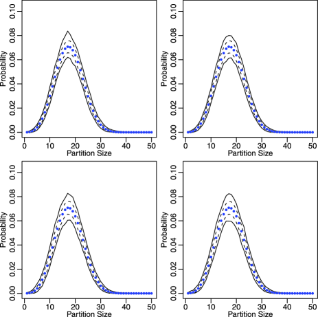
Figure 1: Approximate probabilities of partition sizes of the Poisson Dirichlet process ($\alpha=0.5$, $\theta=1$, $q=1$, $\gamma=0$, $b(x)=0$), $\mathbb{P}\{\aleph(\mathbf{p}_{50})=i\}$ for $i=1,\ldots,50$. Top Left: A.1 algorithm; Top Right: A.2 algorithm; Bottom Left: A.3 algorithm; Bottom Right: A.4 algorithm. The solid bound lines indicate the range of all 10,000 approximates of the probabilities; The dash bound lines indicate the 95% confidence level (2.5% and 97.5% quantiles) of all 10,000 approximates of the probabilities. The dots indicate the true probabilities.

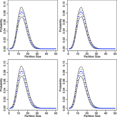
Figure 2: Approximate probabilities of partition sizes of the normalized generalized Gamma process ($\alpha=0.5$, $\theta=1$, $q=0$, $\gamma=0$, $b(x)=1$), $\mathbb{P}\{\aleph(\mathbf{p}_{50})=i\}$ for $i=1,\ldots,50$. Top Left: A.1 algorithm; Top Right: A.2 algorithm; Bottom Left: A.3 algorithm; Bottom Right: A.4 algorithm. The solid bound lines indicate the range of all 10,000 approximates of the probabilities; The dash bound lines indicate the 95% confidence level (2.5% and 97.5% quantiles) of all 10,000 approximates of the probabilities. The dots indicate the true probabilities.

Figure 1 and Table 6 show that for the Poisson–Dirichlet process algorithms A.1 and A.2 result in samples from identical distributions, as the theory would suggest. The MCMC algorithms, A.3 and A.4 also produce similar results to A.1 and A.2 except for the standard errors in Table 6. The standard errors indicate the variability of the MCMC generated samples is generally greater than the exact sequential sampling algorithms, as we would expect. The results for the normalized generalized gamma process shown in Figure 2 and Table 6 point to a similar story as in the Poisson–Dirichlet process.

Finally, we note that it is not necessary to sample $\mathbf{X}_{n}$ to conduct the simulation. It could be done by simply simulating partitions $\mathbf{p}_{n}$ directly instead. It is possible to integrate out all $\mathbf{Y}_{\aleph(\mathbf{p}_{n})}$ from the conditional gbmp urn formula and obtain the weights for partition sampling using the Chinese restaurant process (see Aldous [1], Lo et al. [38] and Pitman [42]).

6 Conclusion and further research

This article has introduced a class of random probability measures based on polynomially and exponentially tilting. We have provided a complete Bayesian analysis of this class of measures with details on the prior and posterior laws and shown that the class is structurally conjugate. We described a conditional Blackwell–MacQueen Pólya urn sampling scheme that simplifies the computational requirements to implement such sampling schemes. The new sampling scheme yields similar answers to more complicated schemes described in the literature.

We also note a general tilting treatment could be considered for any measurable function $h$ on $\mathbb{R}^{+}$ evaluated at the total mass of the corresponding crm in (6). This general class of random probability measures with homogeneous intensity, $\nu(\mathrm{d}x,\mathrm{d}s)=\eta(\mathrm{d}x)\rho(\mathrm{d}s)$, can be shown to be the Poisson–Kingman process (Pitman [41, 42]) by showing that the normalized random probability measure (6) has a Poisson–Kingman partition ($\rho,\gamma$), where $\gamma$ denotes the tilted density of total mass such that $\gamma=f_{\widetilde{T}_{t}}$ (8) and $\rho$ represents the $\sigma$-finite non-atomic intensity measure $\rho(\mathrm{d}s)$. Then, the conditional partition distribution is given by

$$\mathbb{P}(\mathbf{p}_{n}|t)=\int_{(\mathbb{R}^{+})^{\aleph(\mathbf{p}_{n})}}\mathbb{I}_{\{{t}-\sum_{k=1}^{\aleph(\mathbf{p}_{n})}s_{k}>0\}}\frac{f_{\widetilde{T}}({t}-\sum_{k=1}^{\aleph(\mathbf{p}_{n})}s_{k})}{{t}^{n}f_{\widetilde{T}}({t})}\prod_{k=1}^{\aleph(\mathbf{p}_{n})}s_{k}^{n_{k}}\rho(\mathrm{d}s_{k}).$$ (34)

The proof is given in Appendix .5; See also Pitman [41], Lemma 5, page 8, for the related joint distribution of partitions and jumps. Investigation of the properties of this general class of random probably measures and even special cases of (6) is interesting for further research.

==0pt Approximate probabilities of partition sizes of the Poisson Dirichlet process ($\alpha=0.5$, $\theta=1$, $q=1$, $\gamma=0$, $b(x)=0$), $\mathbb{P}\{\aleph(\mathbf{p}_{50})=i\}$ for $i=1,\ldots,50$. First Column: Partition sizes; Second Column: True probability of partition sizes; Third Column: Mean of 10,000 approximates of the probabilities according to algorithm A.1; Fourth Column: Standard error of 10,000 approximates of the probabilities according to algorithm A.1; Fifth Column: Mean of 10,000 approximates of the probabilities according to algorithm A.2; Sixth Column: Standard error of 10,000 approximates of the probabilities according to algorithm A.2; Seventh Column: Mean of 10,000 approximates of the probabilities according to algorithm A.3; Eighth Column: Standard error of 10,000 approximates of the probabilities according to algorithm A.3; Ninth Column: Mean of 10,000 approximates of the probabilities according to algorithm A.4; Tenth Column: Standard error of 10,000 approximates of the probabilities according to algorithm A.4 $\mathbb{P}\{\aleph(\mathbf{p}_{n})=i\}$ A.1 algorithm A.2 algorithm A.3 algorithm A.4 algorithm True Mean of the SE of the Mean of the SE of the Mean of the SE of the Mean of the SE of the $i$ probability approximates approximates approximates approximates approximates approximates approximates approximates 1 0.000063 0.000062 0.000080 0.000063 0.000079 0.000063 0.000088 0.000064 0.000088 2 0.000315 0.000316 0.000179 0.000318 0.000179 0.000313 0.000207 0.000311 0.000207 3 0.000936 0.000933 0.000306 0.000934 0.000308 0.000934 0.000369 0.000936 0.000371 4 0.002139 0.002138 0.000462 0.002133 0.000460 0.002138 0.000567 0.002141 0.000575 5 0.004142 0.004146 0.000639 0.004140 0.000641 0.004147 0.000806 0.004135 0.000807 6 0.007139 0.007129 0.000837 0.007143 0.000836 0.007139 0.001071 0.007131 0.001068 7 0.011258 0.011256 0.001060 0.011242 0.001066 0.011257 0.001351 0.011258 0.001333 8 0.016537 0.016519 0.001274 0.016563 0.001277 0.016536 0.001613 0.016526 0.001610 9 0.022898 0.022916 0.001510 0.022901 0.001502 0.022883 0.001868 0.022890 0.001849 10 0.030135 0.030133 0.001705 0.030123 0.001716 0.030089 0.002075 0.030119 0.002101 11 0.037923 0.037944 0.001923 0.037937 0.001905 0.037893 0.002248 0.037910 0.002311 12 0.045836 0.045829 0.002081 0.045820 0.002121 0.045812 0.002430 0.045901 0.002421 13 0.053388 0.053358 0.002248 0.053434 0.002243 0.053396 0.002515 0.053364 0.002539 14 0.060073 0.060076 0.002407 0.060042 0.002371 0.060038 0.002572 0.060061 0.002600 15 0.065424 0.065423 0.002486 0.065396 0.002497 0.065402 0.002638 0.065415 0.002683 16 0.069059 0.069067 0.002527 0.069071 0.002554 0.069094 0.002677 0.069051 0.002689 17 0.070723 0.070738 0.002575 0.070720 0.002555 0.070754 0.002673 0.070746 0.002684 18 0.070317 0.070311 0.002544 0.070328 0.002558 0.070302 0.002729 0.070290 0.002691 19 0.067906 0.067983 0.002499 0.067911 0.002480 0.067937 0.002692 0.067889 0.002688 20 0.063706 0.063723 0.002443 0.063674 0.002479 0.063756 0.002640 0.063700 0.002636 21 0.058061 0.058033 0.002325 0.058056 0.002349 0.058063 0.002585 0.058066 0.002583

==0pt (Continued) $\mathbb{P}\{\aleph(\mathbf{p}_{n})=i\}$ A.1 algorithm A.2 algorithm A.3 algorithm A.4 algorithm True Mean of the SE of the Mean of the SE of the Mean of the SE of the Mean of the SE of the $i$ probability approximates approximates approximates approximates approximates approximates approximates approximates 22 0.051397 0.051395 0.002197 0.051413 0.002207 0.051427 0.002442 0.051390 0.002478 23 0.044176 0.044171 0.002073 0.044176 0.002040 0.044161 0.002278 0.044206 0.002309 24 0.036847 0.036842 0.001887 0.036834 0.001885 0.036833 0.002103 0.036846 0.002140 25 0.029805 0.029810 0.001705 0.029819 0.001708 0.029830 0.001912 0.029824 0.001945 26 0.023361 0.023352 0.001510 0.023346 0.001515 0.023366 0.001707 0.023369 0.001712 27 0.017724 0.017689 0.001306 0.017739 0.001320 0.017739 0.001477 0.017737 0.001493 28 0.013001 0.012989 0.001127 0.013005 0.001131 0.013004 0.001266 0.013002 0.001259 29 0.009208 0.009204 0.000958 0.009221 0.000963 0.009200 0.001042 0.009208 0.001072 30 0.006287 0.006294 0.000783 0.006280 0.000801 0.006282 0.000859 0.006291 0.000858 31 0.004130 0.004141 0.000645 0.004137 0.000639 0.004129 0.000688 0.004138 0.000690 32 0.002606 0.002606 0.000513 0.002608 0.000514 0.002606 0.000537 0.002603 0.000539 33 0.001575 0.001574 0.000395 0.001571 0.000398 0.001579 0.000423 0.001576 0.000409 34 0.000910 0.000906 0.000302 0.000908 0.000299 0.000911 0.000308 0.000913 0.000312 35 0.000501 0.000502 0.000225 0.000499 0.000223 0.000498 0.000227 0.000502 0.000228 36 0.000261 0.000261 0.000162 0.000261 0.000160 0.000258 0.000163 0.000263 0.000164 37 0.000129 0.000129 0.000113 0.000130 0.000113 0.000128 0.000113 0.000129 0.000114 38 0.000060 0.000061 0.000078 0.000061 0.000079 0.000060 0.000078 0.000059 0.000078 39 0.000026 0.000026 0.000051 0.000027 0.000052 0.000027 0.000052 0.000027 0.000051 40 0.000011 0.000011 0.000032 0.000010 0.000032 0.000011 0.000033 0.000010 0.000032 41 0.000004 0.000004 0.000020 0.000004 0.000020 0.000003 0.000019 0.000004 0.000021 42 0.000001 0.000001 0.000012 0.000001 0.000012 0.000001 0.000012 0.000001 0.000012 43 0.000000 0.000000 0.000006 0.000000 0.000006 0.000000 0.000006 0.000000 0.000006 44 0.000000 0.000000 0.000004 0.000000 0.000004 0.000000 0.000003 0.000000 0.000003 45 0.000000 0.000000 0.000002 0.000000 0.000002 0.000000 0.000002 0.000000 0.000002 46 0.000000 0.000000 0.000000 0.000000 0.000000 0.000000 0.000000 0.000000 0.000000 47 0.000000 0.000000 0.000000 0.000000 0.000000 0.000000 0.000000 0.000000 0.000000 48 0.000000 0.000000 0.000000 0.000000 0.000000 0.000000 0.000000 0.000000 0.000000 49 0.000000 0.000000 0.000000 0.000000 0.000000 0.000000 0.000000 0.000000 0.000000 50 0.000000 0.000000 0.000000 0.000000 0.000000 0.000000 0.000000 0.000000 0.000000

==0pt Approximate of probabilities of partition sizes of the normalized generalized Gamma process ($\alpha=0.5$, $\theta=1$, $q=0$, $\gamma=0$, $b(x)=1$), $\mathbb{P}\{\aleph(\mathbf{p}_{50})=i\}$ for $i=1,\ldots,50$. First Column: Partition sizes; Second Column: True probability of partition sizes; Third Column: Mean of 10,000 approximates of the probabilities according to algorithm A.1; Fourth Column: Standard error of 10,000 approximates of the probabilities according to algorithm A.1; Fifth Column: Mean of 10,000 approximates of the probabilities according to algorithm A.2; Sixth Column: Standard error of 10,000 approximates of the probabilities according to algorithm A.2; Seventh Column: Mean of 10,000 approximates of the probabilities according to algorithm A.3; Eighth Column: Standard error of 10,000 approximates of the probabilities according to algorithm A.3; Ninth Column: Mean of 10,000 approximates of the probabilities according to algorithm A.4; Tenth Column: Standard error of 10,000 approximates of the probabilities according to algorithm A.4 $\mathbb{P}\{\aleph(\mathbf{p}_{n})=i\}$ A.1 algorithm A.2 algorithm A.3 algorithm A.4 algorithm True Mean of the SE of the Mean of the SE of the Mean of the SE of the Mean of the SE of the $i$ probability approximates approximates approximates approximates approximates approximates approximates approximates 1 0.000035 0.000036 0.000059 0.000035 0.000060 0.000035 0.000061 0.000035 0.000061 2 0.000291 0.000294 0.000170 0.000290 0.000170 0.000288 0.000178 0.000293 0.000183 3 0.001234 0.001227 0.000353 0.001238 0.000356 0.001229 0.000389 0.001241 0.000396 4 0.003621 0.003621 0.000599 0.003624 0.000604 0.003620 0.000701 0.003622 0.000703 5 0.008265 0.008274 0.000916 0.008266 0.000909 0.008249 0.001101 0.008262 0.001083 6 0.015684 0.015709 0.001237 0.015683 0.001250 0.015647 0.001554 0.015666 0.001551 7 0.025793 0.025807 0.001598 0.025753 0.001594 0.025786 0.001989 0.025825 0.001997 8 0.037832 0.037827 0.001887 0.037807 0.001896 0.037806 0.002365 0.037843 0.002367 9 0.050538 0.050540 0.002207 0.050498 0.002233 0.050500 0.002645 0.050583 0.002657 10 0.062458 0.062450 0.002393 0.062502 0.002396 0.062445 0.002807 0.062497 0.002823 11 0.072282 0.072260 0.002591 0.072270 0.002557 0.072238 0.002921 0.072246 0.002880 12 0.079070 0.079074 0.002674 0.079123 0.002698 0.079058 0.002932 0.079112 0.002914 13 0.082360 0.082371 0.002745 0.082353 0.002724 0.082412 0.002945 0.082404 0.002924 14 0.082159 0.082126 0.002758 0.082176 0.002764 0.082174 0.002894 0.082143 0.002915 15 0.078842 0.078821 0.002708 0.078836 0.002675 0.078878 0.002847 0.078786 0.002846 16 0.073037 0.072990 0.002618 0.073001 0.002614 0.073106 0.002783 0.073063 0.002804 17 0.065486 0.065510 0.002469 0.065512 0.002465 0.065489 0.002706 0.065455 0.002707 18 0.056942 0.056976 0.002343 0.056984 0.002316 0.056960 0.002585 0.056956 0.002560 19 0.048085 0.048085 0.002165 0.048092 0.002160 0.048113 0.002429 0.048047 0.002398 20 0.039472 0.039478 0.001975 0.039484 0.001980 0.039473 0.002225 0.039428 0.002223 21 0.031516 0.031532 0.001743 0.031496 0.001741 0.031529 0.002037 0.031498 0.002037

==0pt (Continued) $\mathbb{P}\{\aleph(\mathbf{p}_{n})=i\}$ A.1 algorithm A.2 algorithm A.3 algorithm A.4 algorithm True Mean of the SE of the Mean of the SE of the Mean of the SE of the Mean of the SE of the $i$ probability approximates approximates approximates approximates approximates approximates approximates approximates 22 0.024480 0.024454 0.001541 0.024485 0.001554 0.024485 0.001765 0.024466 0.001769 23 0.018499 0.018503 0.001338 0.018488 0.001361 0.018484 0.001535 0.018502 0.001544 24 0.013595 0.013589 0.001155 0.013583 0.001166 0.013584 0.001308 0.013604 0.001307 25 0.009711 0.009716 0.000978 0.009696 0.000982 0.009703 0.001091 0.009714 0.001110 26 0.006738 0.006750 0.000824 0.006743 0.000819 0.006738 0.000907 0.006725 0.000910 27 0.004537 0.004544 0.000670 0.004547 0.000676 0.004544 0.000738 0.004538 0.000732 28 0.002960 0.002961 0.000545 0.002959 0.000547 0.002958 0.000593 0.002960 0.000585 29 0.001870 0.001866 0.000434 0.001867 0.000432 0.001870 0.000460 0.001872 0.000463 30 0.001141 0.001144 0.000337 0.001144 0.000338 0.001136 0.000354 0.001146 0.000359 31 0.000672 0.000672 0.000260 0.000674 0.000257 0.000667 0.000269 0.000673 0.000273 32 0.000381 0.000379 0.000195 0.000380 0.000195 0.000381 0.000203 0.000384 0.000203 33 0.000207 0.000207 0.000144 0.000206 0.000143 0.000208 0.000148 0.000205 0.000147 34 0.000108 0.000108 0.000105 0.000108 0.000104 0.000107 0.000105 0.000107 0.000105 35 0.000054 0.000053 0.000073 0.000053 0.000072 0.000054 0.000075 0.000053 0.000073 36 0.000025 0.000025 0.000050 0.000025 0.000051 0.000026 0.000052 0.000025 0.000050 37 0.000011 0.000011 0.000033 0.000012 0.000034 0.000011 0.000033 0.000012 0.000034 38 0.000005 0.000005 0.000023 0.000005 0.000022 0.000005 0.000022 0.000005 0.000022 39 0.000002 0.000002 0.000014 0.000002 0.000014 0.000002 0.000013 0.000002 0.000014 40 0.000001 0.000001 0.000008 0.000001 0.000009 0.000001 0.000009 0.000001 0.000008 41 0.000000 0.000000 0.000006 0.000000 0.000005 0.000000 0.000005 0.000000 0.000005 42 0.000000 0.000000 0.000003 0.000000 0.000002 0.000000 0.000002 0.000000 0.000002 43 0.000000 0.000000 0.000001 0.000000 0.000001 0.000000 0.000001 0.000000 0.000001 44 0.000000 0.000000 0.000000 0.000000 0.000000 0.000000 0.000000 0.000000 0.000000 45 0.000000 0.000000 0.000000 0.000000 0.000000 0.000000 0.000000 0.000000 0.000000 46 0.000000 0.000000 0.000000 0.000000 0.000000 0.000000 0.000000 0.000000 0.000000 47 0.000000 0.000000 0.000000 0.000000 0.000000 0.000000 0.000000 0.000000 0.000000 48 0.000000 0.000000 0.000000 0.000000 0.000000 0.000000 0.000000 0.000000 0.000000 49 0.000000 0.000000 0.000000 0.000000 0.000000 0.000000 0.000000 0.000000 0.000000 50 0.000000 0.000000 0.000000 0.000000 0.000000 0.000000 0.000000 0.000000 0.000000

Finally, we note that the applications of Bayesian non-parametric mixture models in Bayesian statistics is steadily increasing (see Lo [36]; James [18]; Ishwaran and James [16, 17]; James et al. [22]; Lijoi et al. [31, 32, 34]). In particular, time series model mixing over random probability measures has been considered recently in Griffin and Steel [13], Lau and So [29, 30] and Lau and Cripps [28]. Often in mixture models over the normalized tilted crm, it is necessary to consider a collection of latent variables, which is a sample of the normalized tilted crm but these latent variables are not observed directly. In fact, sampling latent variables is essential for approximating estimates of parameters of interest that are functions of the latent variables, $\mathbf{X}_{n}$ because of the high cardinality of the posterior distribution due to combinatorial property of the latent variables. As a result, sampling schemes for $\mathbf{X}_{n}$ are required for estimation based on the conditional Blackwell–MacQueen Pólya urn formula and the distributions of $\mathbf{X}_{n}$ and partitions $\mathbf{p}_{n}$. In this article, we have provided the marginal distributions of $\mathbf{X}_{n}$ and $\mathbf{p}_{n}$, both conditional and unconditional on $U_{n}$, that are essential elements in implementing mixture models over the normalized tilted crm.

Appendix

.1 Proof of Theorem 3.1

Consider the joint distribution of $(\widetilde{\mu}_{t},\mathbf{X}_{n})$, which is given by (14) and (15), that is

$$\mathcal{P}_{\widetilde{\mu}_{t},\mathbf{X}_{n}}(A,B_{1},\ldots,B_{n})=\frac{1}{E[h^{\prime}(\widetilde{\mu}(\mathbb{X}))\widetilde{\mu}(\mathbb{X})^{-q}]}\int_{A}\frac{h^{\prime}(\mu(\mathbb{X}))}{\mu(\mathbb{X})^{n+q}}\Biggl{(}\prod_{i=1}^{n}\mu(B_{i})\Biggr{)}\mathcal{P}_{\widetilde{\mu}}(\mathrm{d}\mu).$$ (1)

In (1), the crm $\widetilde{\mu}(\cdot)$ is now replaced by the linear functional of the Poisson process $\int_{\mathbb{R}^{+}}sN(\cdot,\mathrm{d}s)$ on $\mathbb{X}$ (4). Following by writing the right hand side of (1) without the integrals, that is given by

$$\frac{h^{\prime}(\int_{\mathbb{X}\times\mathbb{R}^{+}}sN(\mathrm{d}x,\mathrm{d}s))}{(\int_{\mathbb{X}\times\mathbb{R}^{+}}sN(\mathrm{d}x,\mathrm{d}s))^{n+q}}\Biggl{(}\prod_{i=1}^{n}s_{i}N(\mathrm{d}x_{i},\mathrm{d}s_{i})\Biggr{)}\mathcal{P}_{N}(\mathrm{d}N),$$ (2)

where this Poisson process $N$ has distribution denoted by $\mathcal{P}_{N}$, has the intensity measure $\nu$ same as that of $\widetilde{\mu}$ (4), and belong to the set in $\mathcal{B}(\mathcal{M}_{\mathbb{X}\times\mathbb{R}^{+}})$ corresponding to the set $A$ that $\mu\in A\in\mathcal{B}(\mathcal{M}_{\mathbb{X}})$. Here $(x_{i},s_{i})$ for $i=1,\ldots,n$ represent the points generated from the Poisson process $N$. For $k=1,\ldots,\aleph(\mathbf{p}_{n})$, $(Y_{k},J_{k})$ denotes the distinct points of the $(x_{i},s_{i})$’s and $\aleph(\mathbf{p}_{n})$ denotes the number of the distinct points. In addition, we take $\{J_{1},\ldots,J_{\aleph(\mathbf{p}_{n})}\}$ to be the augmented variables. We then apply the Fubini theorem following from an application of Lemma 2.2 of James [18], page 8 (see also James [18] for some detail discussions), to yield the joint distribution of $N$, $\mathbf{p}_{n}$ and $(Y_{k},J_{k})$ for $k=1,\ldots,\aleph(\mathbf{p}_{n})$, which is given by (2) without the proportional constant,

$$\frac{h^{\prime}(\int_{\mathbb{X}\times\mathbb{R}^{+}}sN^{(\mathbf{X}_{n})}(\mathrm{d}x,\mathrm{d}s))}{(\int_{\mathbb{X}\times\mathbb{R}^{+}}sN^{(\mathbf{X}_{n})}(\mathrm{d}x,\mathrm{d}s))^{n+q}}\mathcal{P}_{N}(\mathrm{d}N)\prod_{k=1}^{\aleph(\mathbf{p}_{n})}\eta(\mathrm{d}Y_{k})s_{k}^{n_{k}}\rho_{Y_{k}}(\mathrm{d}s_{k}),$$ (3)

where $N^{(\mathbf{X}_{n})}\stackrel{{\scriptstyle d}}{{=}}N+\sum_{k=1}^{\aleph(\mathbf{p}_{n})}\delta_{(Y_{k},J_{k}^{(\mathbf{X}_{n})})}$. Here the distribution of $N^{(\mathbf{X}_{n})}$ is identical to the distribution of the sum over a Poisson process $N$ and the fixed points of discontinuity at $(Y_{k},J_{k}^{(\mathbf{X}_{n})})$. The Poisson process $N$ has the intensity measure $\nu$ and be independent of $(Y_{k},J_{k}^{(\mathbf{X}_{n})})$ for $k=1,\ldots,\aleph(\mathbf{p}_{n})$. The pairs $(Y_{k},J_{k}^{(\mathbf{X}_{n})})$ for $k=1,\ldots,\aleph(\mathbf{p}_{n})$ and $\mathbf{p}_{n}$ has the joint distribution $\prod_{k=1}^{\aleph(\mathbf{p}_{n})}[\eta(\mathrm{d}Y_{k})\times\mathbb{P}(J_{k}^{(\mathbf{X}_{n})}\in\mathrm{d}s_{k})\times\tau_{n_{k},Y_{k}}(0)]$ where $\mathbb{P}(J_{k}^{(\mathbf{X}_{n})}\in\mathrm{d}s_{k})=s_{k}^{n_{k}}\rho_{Y_{k}}(\mathrm{d}s_{k})/\int_{\mathbb{R}^{+}}s_{k}^{n_{k}}\rho_{Y_{k}}(\mathrm{d}s_{k})$ and $\tau_{n_{k},Y_{k}}(0)$ defined in (27). The distribution of $N^{(\mathbf{X}_{n})}$ now is denoted by $\mathcal{P}_{N}^{(\mathbf{X}_{n})}$, so (3) could be reduced to

$$\frac{h^{\prime}(\int_{\mathbb{X}\times\mathbb{R}^{+}}sN(\mathrm{d}x,\mathrm{d}s))}{(\int_{\mathbb{X}\times\mathbb{R}^{+}}sN(\mathrm{d}x,\mathrm{d}s))^{n+q}}\mathcal{P}_{N}^{(\mathbf{X}_{n})}(\mathrm{d}N).$$ (4)

The Poisson linear functional appears in (4), $\int_{\mathbb{R}^{+}}sN^{(\mathbf{X}_{n})}(\mathrm{d}x,\mathrm{d}s)$ ($=:\widetilde{\mu}^{(\mathbf{X}_{n})}(\mathrm{d}x)$), is a completely random measure according to (1) (see also Daley and Vere-Jones [8], Theorem 10.1.III, page 79), such that

$$\widetilde{\mu}^{(\mathbf{X}_{n})}(\mathrm{d}x)\stackrel{{\scriptstyle d}}{{=}}\int_{\mathbb{R}^{+}}sN(\mathrm{d}x,\mathrm{d}s)+\sum_{k=1}^{\aleph(\mathbf{p}_{n})}J_{k}^{(\mathbf{X}_{n})}\delta_{Y_{k}}(\mathrm{d}x)\stackrel{{\scriptstyle d}}{{=}}\widetilde{\mu}(\mathrm{d}x)+\sum_{k=1}^{\aleph(\mathbf{p}_{n})}J_{k}^{(\mathbf{X}_{n})}\delta_{Y_{k}}(\mathrm{d}x),$$ (5)

where $\widetilde{\mu}$ denote a crm (4) derived from the Poisson process $N$. So, the total mass $\widetilde{\mu}^{(\mathbf{X}_{n})}(\mathbb{X})$ in (4) is given by

$$\widetilde{\mu}^{(\mathbf{X}_{n})}(\mathbb{X})\stackrel{{\scriptstyle d}}{{=}}\widetilde{\mu}(\mathbb{X})+\sum_{k=1}^{\aleph(\mathbf{p}_{n})}J_{k}^{(\mathbf{X}_{n})}.$$ (6)

This immediately reveals the distribution of the tilted completely random measure, $\widetilde{\mu}^{(\mathbf{X}_{n})}_{t}$ (Definition 2.1), that is $\mathcal{P}_{\widetilde{\mu}_{t}}^{(\mathbf{X}_{n})}(\mathrm{d}\mu)\propto\frac{h^{\prime}(\mu^{(\mathbf{X}_{n})}(\mathbb{X}))}{(\mu^{(\mathbf{X}_{n})}(\mathbb{X}))^{n+q}}\mathcal{P}_{\widetilde{\mu}}^{(\mathbf{X}_{n})}(\mathrm{d}\mu)$. Lastly, the distributional identity derived from the a sample $\widetilde{\mu}^{(\mathbf{X}_{n})}_{t}$ from $\mathcal{P}_{\widetilde{\mu}_{t}}^{(\mathbf{X}_{n})}$, $G^{(\mathbf{X}_{n})}(\cdot)\stackrel{{\scriptstyle d}}{{=}}\widetilde{\mu}^{(\mathbf{X}_{n})}_{t}(\cdot)/\widetilde{\mu}^{(\mathbf{X}_{n})}_{t}(\mathbb{X})$ on $\mathbb{X}$ is obtained by the same arguments in the proof of Theorem 2 of James et al. [22], page 96. Thus, the proof is complete.

.2 Proof of Theorem 3.2

Following the proof of Theorem 3.1 from the beginning to (3) with chosen $h^{\prime}(x)=\mathrm{e}^{-\gamma x}$. Using the facts from (5) and (6), the distribution (3) becomes

$$\frac{\mathrm{e}^{-\gamma(\mu(\mathbb{X})+\sum_{k=1}^{\aleph(\mathbf{p}_{n})}s_{k})}}{(\mu(\mathbb{X})+\sum_{k=1}^{\aleph(\mathbf{p}_{n})}s_{k})^{n+q}}\mathcal{P}_{\widetilde{\mu}}(\mathrm{d}\mu)\prod_{k=1}^{\aleph(\mathbf{p}_{n})}\eta(\mathrm{d}Y_{k})s_{k}^{n_{k}}\rho_{Y_{k}}(\mathrm{d}s_{k}).$$ (7)

This is the joint distribution of $\widetilde{\mu}$, $\mathbf{p}_{n}$ and $Y_{k}$ for $k=1,\ldots,\aleph(\mathbf{p}_{n})$. Then we apply the gamma identity (16) on the term $(\mu(\mathbb{X})+\sum_{k=1}^{\aleph(\mathbf{p}_{n})}s_{k})^{-(n+q)}$ in (7)

$$\frac{1}{(\mu(\mathbb{X})+\sum_{k=1}^{\aleph(\mathbf{p}_{n})}s_{k})^{n+q}}=\frac{1}{\Gamma(n+q)}\int_{\mathbb{R}^{+}}\mathrm{e}^{-(\mu(\mathbb{X})+\sum_{k=1}^{\aleph(\mathbf{p}_{n})}s_{k})u}u^{n+q-1}\,\mathrm{d}u,$$ (8)

Here the augmented variable $U_{n}$ is introduced due to the gamma identity. Incorporating (7) with (8) and omiting the integrals, it turns out that the following is the joint distribution of $U_{n}$, $\widetilde{\mu}$, $\mathbf{p}_{n}$ and $Y_{k}$ for $k=1,\ldots,\aleph(\mathbf{p}_{n})$,

$$\mathrm{e}^{-(\gamma+u)\mu(\mathbb{X})}\mathcal{P}_{\widetilde{\mu}}(\mathrm{d}\mu)\frac{u^{n+q-1}}{\Gamma(n+q)}\prod_{k=1}^{\aleph(\mathbf{p}_{n})}\eta(\mathrm{d}Y_{k})s_{k}^{n_{k}}\mathrm{e}^{-s_{k}(\gamma+u)}\rho_{Y_{k}}(\mathrm{d}s_{k})\,\mathrm{d}u.$$ (9)

The disintegration between terms in $\mathrm{e}^{-(\gamma+u)\mu(\mathbb{X})}$ and $\mathcal{P}_{\widetilde{\mu}}(\mathrm{d}\mu)$ in (9) yields $\mathrm{e}^{-\psi_{0}(\gamma+u)}$ and $\mathcal{P}_{\widetilde{\mu}^{(u)}}(\mathrm{d}\mu)$ where $\psi_{0}$ is defined in (9) and the completely random measure $\widetilde{\mu}^{(u)}$ has the intensity measure $\nu^{(u)}(\mathrm{d}x,\mathrm{d}s)=\eta(\mathrm{d}x)\mathrm{e}^{-(\gamma+u)s}\rho_{x}(\mathrm{d}s)$. Then, (9) turns out to be

$$\mathcal{P}_{\widetilde{\mu}^{(u)}}(\mathrm{d}\mu)\mathrm{e}^{-\psi_{0}(\gamma+u)}\frac{u^{n+q-1}}{\Gamma(n+q)}\prod_{k=1}^{\aleph(\mathbf{p}_{n})}\eta(\mathrm{d}Y_{k})s_{k}^{n_{k}}\mathrm{e}^{-s_{k}(\gamma+u)}\rho_{Y_{k}}(\mathrm{d}s_{k})\,\mathrm{d}u.$$ (10)

So, conditional on $U_{n}$ and $\mathbf{X}_{n}$, the process $\widetilde{\mu}^{(U_{n})}+\sum_{k=1}^{\aleph(\mathbf{p}_{n})}J_{k}^{(U_{n},\mathbf{X}_{n})}\delta_{Y_{k}}$ is a completely random measure (1) (see also Daley and Vere-Jones [8], page 79, Theorem 10.1.III) such that

$$\widetilde{\mu}^{(U_{n},\mathbf{X}_{n})}(\mathrm{d}x)\stackrel{{\scriptstyle d}}{{=}}\widetilde{\mu}^{(U_{n})}(\mathrm{d}x)+\sum_{k=1}^{\aleph(\mathbf{p}_{n})}J_{k}^{(U_{n},\mathbf{X}_{n})}\delta_{Y_{k}}(\mathrm{d}x),$$ (11)

where each $J_{k}^{(U_{n},\mathbf{X}_{n})}$ has the density $\mathbb{P}(J_{k}^{(U_{n},\mathbf{X}_{n})}\in\mathrm{d}s)=\frac{s^{n_{k}}\mathrm{e}^{-s(\gamma+U_{n})}\rho_{Y_{k}}(\mathrm{d}s)}{\int_{\mathbb{R}^{+}}s^{n_{k}}\mathrm{e}^{-s(\gamma+U_{n})}\rho_{Y_{k}}(\mathrm{d}s)}$ for $k=1,\ldots,\allowbreak\aleph(\mathbf{p}_{n})$ and $\{J_{1}^{(U_{n},\mathbf{X}_{n})},\ldots,J_{\aleph(\mathbf{p}_{n})}^{(U_{n},\mathbf{X}_{n})}\}$ are conditionally independent. Furthermore, conditional on $U_{n}$, $\widetilde{\mu}^{(U_{n})}$ and $\{J_{1}^{(U_{n},\mathbf{X}_{n})},\ldots,J_{\aleph(\mathbf{p}_{n})}^{(U_{n},\mathbf{X}_{n})}\}$ are independent. Lastly the distributional identity $\widetilde{G}^{(U_{n},\mathbf{X}_{n})}(\cdot)\stackrel{{\scriptstyle d}}{{=}}\widetilde{\mu}^{(U_{n},\mathbf{X}_{n})}(\cdot)/\widetilde{\mu}^{(U_{n},\mathbf{X}_{n})}(\mathbb{X})$ is obtained by the same arguments in the proof of Theorem 2 of James et al. [22], page 96, and $\widetilde{G}^{(U_{n},\mathbf{X}_{n})}$ is a normalized completely random measure. Thus, the proof is complete.

.3 Proof of Proposition 3.1

Following the definition of the predictive distribution,

$$\mathbb{P}\{X_{n+1}\in\mathrm{d}x|\mathbf{X}_{n}\}=\int_{\mathbb{R}^{+}}E\bigl{[}\widetilde{G}^{(U_{n},\mathbf{X}_{n})}(\mathrm{d}x)|\mathbf{X}_{n},U_{n}=u\bigr{]}f_{U_{n}|\mathbf{X}_{n}}(u)\,\mathrm{d}u,$$ (12)

and using the result from Theorem 3.2, the expectation (12) inside the integral is given by

$$E\bigl{[}\widetilde{G}^{(U_{n},\mathbf{X}_{n})}(\mathrm{d}x)|\mathbf{X}_{n},U_{n}\bigr{]}$$

$$\quad=E\biggl{[}\frac{\widetilde{\mu}^{(U_{n})}(\mathrm{d}x)}{\widetilde{\mu}^{(U_{n})}(\mathbb{X})+\sum_{k^{\prime}=1}^{\aleph(\mathbf{p}_{n})}J_{k^{\prime}}^{(U_{n},\mathbf{X}_{n})}}\Big{|}\mathbf{X}_{n},U_{n}\biggr{]}$$ (13)

$$\qquad{}+\sum_{k=1}^{\aleph(\mathbf{p}_{n})}E\biggl{[}\frac{J_{k}^{(U_{n},\mathbf{X}_{n})}}{\widetilde{\mu}^{(U_{n})}(\mathbb{X})+\sum_{k^{\prime}=1}^{\aleph(\mathbf{p}_{n})}J_{k^{\prime}}^{(U_{n},\mathbf{X}_{n})}}\Big{|}\mathbf{X}_{n},U_{n}\biggr{]}\delta_{Y_{k}}(\mathrm{d}x).$$

We use Theorem 3.2 to obtain the explicit results of the expectations (.3) according to the conditional distributions of $\widetilde{\mu}^{(U_{n})}$ and $J_{k}^{(U_{n},\mathbf{X}_{n})}$ for $k=1,\ldots,\aleph(\mathbf{p}_{n})$. There are two expected values (.3) considered in the following. Firstly, an exponential identity in the first integral of (.3) yields,

$$E\biggl{[}\frac{\widetilde{\mu}^{(U_{n})}(\mathrm{d}x)}{\mu^{(U_{n})}(\mathbb{X})+\sum_{k^{\prime}=1}^{\aleph(\mathbf{p}_{n})}J_{k^{\prime}}^{(U_{n},\mathbf{X}_{n})}}\Big{|}\mathbf{X}_{n},U_{n}\biggr{]}$$

$$\quad=\int_{\mathbb{R}^{+}}E\Biggl{[}\widetilde{\mu}^{(U_{n})}(\mathrm{d}x)\mathrm{e}^{-z\widetilde{\mu}^{(U_{n})}(\mathbb{X})}\prod_{k^{\prime}=1}^{\aleph(\mathbf{p}_{n})}\mathrm{e}^{-zJ_{k^{\prime}}^{(U_{n},\mathbf{X}_{n})}}\Big{|}\mathbf{X}_{n},U_{n}\Biggr{]}\mathrm{d}z.$$

We apply a change of measure on $\widetilde{\mu}^{(U_{n})}$ and compute directly on the expectation with respect to $J_{k}^{(U_{n},\mathbf{X}_{n})}$ for $k=1,\ldots,\aleph(\mathbf{p}_{n})$, (.3) turns out to be

$$\eta(\mathrm{d}x)\times\int_{\mathbb{R}^{+}}\mathrm{e}^{-\psi_{\gamma+U_{n}}(z)}\tau_{1,x}(\gamma+z+U_{n})\prod_{k=1}^{\aleph(\mathbf{p}_{n})}\frac{\tau_{n_{k},Y_{k}}(\gamma+z+U_{n})}{\tau_{n_{k},Y_{k}}(\gamma+U_{n})}\,\mathrm{d}z.$$ (15)

Marginalizing over $U_{n}$ on (15) is given by

$$\int_{\mathbb{R}^{+}}E\biggl{[}\frac{\widetilde{\mu}^{(U_{n})}(\mathrm{d}x)}{\widetilde{\mu}^{(U_{n})}(\mathbb{X})+\sum_{k^{\prime}=1}^{\aleph(\mathbf{p}_{n})}J_{k^{\prime}}^{(U_{n},\mathbf{X}_{n})}}|\mathbf{X}_{n},U_{n}\biggr{]}f_{U_{n}|\mathbf{X}_{n}}(u)\,\mathrm{d}u$$

$$\quad=\eta(\mathrm{d}x)\times\int_{\mathbb{R}^{+}\times\mathbb{R}^{+}}\mathrm{e}^{-\psi_{\gamma+u}(z)}\tau_{1,x}(\gamma+z+u)$$ (16)

$$\hskip 86.0pt{}\times\frac{\mathrm{e}^{-\psi_{0}(\gamma+u)}\prod_{k=1}^{\aleph(\mathbf{p}_{n})}\tau_{n_{k},Y_{k}}(\gamma+z+u)u^{n+q-1}}{\int_{\mathbb{R}^{+}}\mathrm{e}^{-\psi_{0}(\gamma+u)}\prod_{k=1}^{\aleph(\mathbf{p}_{n})}\tau_{n_{k},Y_{k}}(\gamma+u)u^{n+q-1}\,\mathrm{d}u}\,\mathrm{d}u\,\mathrm{d}z.$$

Taking the equality $\psi_{0}(\gamma+z+u)=\psi_{\gamma+u}(z)+\psi_{0}(\gamma+u)$ and transforming the upper integral with $(w,v)=(u+z,u)$, (.3) becomes

$$\eta(\mathrm{d}x)\times\frac{\int_{\mathbb{R}^{+}}\mathrm{e}^{-\psi_{0}(\gamma+w)}\tau_{1,x}(\gamma+w)\prod_{k=1}^{\aleph(\mathbf{p}_{n})}\tau_{n_{k},Y_{k}}(\gamma+w){w^{n+q}}/({n+q})\,\mathrm{d}w}{\int_{\mathbb{R}^{+}}\mathrm{e}^{-\psi_{0}(\gamma+u)}\prod_{k=1}^{\aleph(\mathbf{p}_{n})}\tau_{n_{k},Y_{k}}(\gamma+u)u^{n+q-1}\,\mathrm{d}u}$$

$$\quad=\eta(\mathrm{d}x)\times\frac{1}{n+q}\int_{\mathbb{R}^{+}}\tau_{1,x}(\gamma+u)uf_{U_{n}|\mathbf{X}_{n}}(u)\,\mathrm{d}u.$$

Now consider the second expectation of (.3). As before, an exponential identity in the second integral yields,

$$E\biggl{[}\frac{J_{k}^{(U_{n},\mathbf{X}_{n})}}{\mu^{(U_{n})}(\mathbb{X})+\sum_{k^{\prime}=1}^{\aleph(\mathbf{p}_{n})}J_{k^{\prime}}^{(U_{n},\mathbf{X}_{n})}}\Big{|}\mathbf{X}_{n},U_{n}\biggr{]}$$

(17)

$$\quad=\int_{\mathbb{R}^{+}}E\Biggl{[}J_{k}^{(U_{n},\mathbf{X}_{n})}\mathrm{e}^{-z\mu^{(U_{n})}(\mathbb{X})}\prod_{k^{\prime}=1}^{\aleph(\mathbf{p}_{n})}\mathrm{e}^{-zJ_{k^{\prime}}^{(U_{n},\mathbf{X}_{n})}}\Big{|}\mathbf{X}_{n},U_{n}\Biggr{]}\,\mathrm{d}z.$$

By direct computation, (.3) turns out to be

$$\int_{\mathbb{R}^{+}}\mathrm{e}^{-\psi_{\gamma+U_{n}}(z)}\frac{\tau_{n_{k}+1,Y_{k}}(\gamma+z+U_{n})}{\tau_{n_{k},Y_{k}}(\gamma+U_{n})}\prod_{k^{\prime}=1,k^{\prime}\neq k}^{\aleph(\mathbf{p}_{n})}\frac{\tau_{n_{k^{\prime}},Y_{k^{\prime}}}(\gamma+z+U_{n})}{\tau_{n_{k^{\prime}},Y_{k^{\prime}}}(\gamma+U_{n})}\,\mathrm{d}z.$$ (18)

Marginalizing over $U_{n}$ on (18) is given by

$$\int_{\mathbb{R}^{+}}E\biggl{[}\frac{J_{k}^{(U_{n},\mathbf{X}_{n})}}{\widetilde{\mu}^{(U_{n})}(\mathbb{X})+\sum_{k^{\prime}=1}^{\aleph(\mathbf{p}_{n})}J_{k^{\prime}}^{(U_{n},\mathbf{X}_{n})}}\Big{|}\mathbf{X}_{n},U_{n}\biggr{]}f_{U_{n}|\mathbf{X}_{n}}(u)\,\mathrm{d}u$$

$$\quad=\int_{\mathbb{R}^{+}\times\mathbb{R}^{+}}\mathrm{e}^{-\psi_{\gamma+u}(z)}\tau_{n_{k}+1,Y_{k}}(\gamma+z+u)$$ (19)

$$\hskip 51.0pt{}\times\frac{\mathrm{e}^{-\psi_{0}(\gamma+u)}\prod_{k^{\prime}=1,k^{\prime}\neq k}^{\aleph(\mathbf{p}_{n})}\tau_{n_{k^{\prime}},Y_{k^{\prime}}}(\gamma+z+u)u^{n+q-1}}{\int_{\mathbb{R}^{+}}\mathrm{e}^{-\psi_{0}(\gamma+u)}\prod_{k^{\prime}=1}^{\aleph(\mathbf{p}_{n})}\tau_{n_{k^{\prime}},Y_{k^{\prime}}}(\gamma+u)u^{n+q-1}\,\mathrm{d}u}\,\mathrm{d}u\,\mathrm{d}z.$$

Taking the equality $\psi_{0}(\gamma+z+u)=\psi_{\gamma+u}(z)+\psi_{0}(\gamma+u)$ and transforming the upper integral with $(w,v)=(u+z,u)$, (.3) becomes

$$\frac{\int_{\mathbb{R}^{+}}\mathrm{e}^{-\psi_{0}(\gamma+w)}\tau_{n_{k}+1,Y_{k}}(\gamma+w)\prod_{k^{\prime}=1,k^{\prime}\neq k}^{\aleph(\mathbf{p}_{n})}\tau_{n_{k^{\prime}},Y_{k^{\prime}}}(\gamma+w){w^{n+q}}/({n+q})\,\mathrm{d}w}{\int_{\mathbb{R}^{+}}\mathrm{e}^{-\psi_{0}(\gamma+u)}\prod_{k^{\prime}=1}^{\aleph(\mathbf{p}_{n})}\tau_{n_{k^{\prime}},Y_{k^{\prime}}}(\gamma+u)u^{n+q-1}\,\mathrm{d}u}$$

(20)

$$\quad=\frac{1}{n+q}\int_{\mathbb{R}^{+}}\frac{\tau_{n_{k}+1,Y_{k}}(\gamma+u)}{\tau_{n_{k},Y_{k}}(\gamma+u)}uf_{U_{n}|\mathbf{X}_{n}}(u)\,\mathrm{d}u.$$

We conclude that the predictive distribution for $X_{n+1}$ given $\mathbf{X}_{n}=\{X_{1},\ldots,X_{n}\}$ is given by

$$\mathbb{P}\{X_{n+1}\in\mathrm{d}x|\mathbf{X}_{n}\} = \frac{1}{n+q}\int_{\mathbb{R}^{+}}u\tau_{1,x}(\gamma+u)f_{U_{n}|\mathbf{X}_{n}}(u)\,\mathrm{d}u\times\eta(\mathrm{d}x)$$

$${}+\sum_{k=1}^{\aleph(\mathbf{p}_{n})}\frac{1}{n+q}\int_{\mathbb{R}^{+}}u\frac{\tau_{n_{k}+1,Y_{k}}(\gamma+u)}{\tau_{n_{k},Y_{k}}(\gamma+u)}f_{U_{n}|\mathbf{X}_{n}}(u)\,\mathrm{d}u\times\delta_{Y_{k}}(\mathrm{d}x).\quad$$

This representation is analogous to James et al. [22]. In fact, we prefer an intuitive representation for this predictive distribution for the next proof of the conditional case. A representation of the predictive distribution is given by

$$\mathbb{P}\{X_{n+1}\in\mathrm{d}x|\mathbf{X}_{n}\}=\frac{\omega_{n,\aleph(\mathbf{p}_{n})+1}(x)}{\phi(\mathbf{X}_{n})}\eta(\mathrm{d}x)+\sum_{k=1}^{\aleph(\mathbf{p}_{n})}\frac{\omega_{n,k}(Y_{k})}{\phi(\mathbf{X}_{n})}\delta_{Y_{k}}(\mathrm{d}x),$$ (22)

where

$$\omega_{n,\aleph(\mathbf{p}_{n})+1}(x) = \int_{\mathbb{R}^{+}}u\tau_{1,x}(\gamma+u)f_{U_{n}|\mathbf{X}_{n}}(u)\,\mathrm{d}u,$$

$$\omega_{n,k}(Y_{k}) = \int_{\mathbb{R}^{+}}u\frac{\tau_{n_{k}+1,Y_{k}}(\gamma+u)}{\tau_{n_{k},Y_{k}}(\gamma+u)}f_{U_{n}|\mathbf{X}_{n}}(u)\,\mathrm{d}u,$$

$$\phi(\mathbf{X}_{n}) = \int_{\mathbb{X}}\omega_{n,\aleph(\mathbf{p}_{n})+1}(x)\eta(\mathrm{d}x)+\sum_{k=1}^{\aleph(\mathbf{p}_{n})}\omega_{n,k}(Y_{k})=n+q.$$

Clearly, we could write (.3) or (22) as an expectation with respect to the distribution $U_{n}$ given $\mathbf{X}_{n}$, $\mathbb{P}\{X_{n+1}\in\mathrm{d}x|\mathbf{X}_{n}\}=E[\mathbb{P}\{X_{n+1}\in\mathrm{d}x|\mathbf{X}_{n},U_{n}\}|\mathbf{X}_{n}]$. However, the term $\mathbb{P}\{X_{n+1}\in\mathrm{d}x|\mathbf{X}_{n},U_{n}\}$ might not be a proper distribution. We suggest the following expectation instead with respect to the distribution $\widetilde{U}_{n}$ given $\mathbf{X}_{n}$, $\mathbb{P}\{X_{n+1}\in\mathrm{d}x|\mathbf{X}_{n}\}=E[\mathbb{P}\{X_{n+1}\in\mathrm{d}x|\mathbf{X}_{n},\widetilde{U}_{n}\}|\mathbf{X}_{n}]$. So conditional on $\widetilde{U}_{n}$, the predictive distribution is given by

$$\mathbb{P}\{X_{n+1}\in\mathrm{d}x|\mathbf{X}_{n},\widetilde{U}_{n}\} = \frac{\omega_{n,\aleph(\mathbf{p}_{n})+1}(\widetilde{U}_{n},x)}{\phi(\widetilde{U}_{n},\mathbf{X}_{n})}\eta(\mathrm{d}x)+\sum_{k=1}^{\aleph(\mathbf{p}_{n})}\frac{\omega_{n,k}(\widetilde{U}_{n},Y_{k})}{\phi(\widetilde{U}_{n},\mathbf{X}_{n})}\delta_{Y_{k}}(\mathrm{d}x),$$

$$\phi(u,\mathbf{X}_{n}) = \int_{\mathbb{X}}\omega_{n,\aleph(\mathbf{p}_{n})+1}(u,x)\eta(\mathrm{d}x)+\sum_{k=1}^{\aleph(\mathbf{p}_{n})}\omega_{n,k}(u,Y_{k}),$$

$$\omega_{n,\aleph(\mathbf{p}_{n})+1}(u,x) = u\tau_{1,x}(\gamma+u),$$

$$\omega_{n,k}(u,Y_{k}) = u\frac{\tau_{n_{k}+1,Y_{k}}(\gamma+u)}{\tau_{n_{k},Y_{k}}(\gamma+u)},\qquad k=1,\ldots,\aleph(\mathbf{p}_{n})\quad\mbox{and}$$

$$f_{\widetilde{U}_{n}|\mathbf{X}_{n}}(u) = \frac{\phi(u,\mathbf{X}_{n})}{E[\phi(U_{n},\mathbf{X}_{n})|\mathbf{X}_{n}]}f_{U_{n}|\mathbf{X}_{n}}(u).$$

Lastly, the following equality can be achieved by inspection of (.3) and (22), $\phi(\mathbf{X}_{n})=E[\phi(U_{n}|\mathbf{X}_{n})|\mathbf{X}_{n}]=n+q$ and the following equalities can be obtained according to the definitions, $\omega_{n,\aleph(\mathbf{p}_{n})+1}(x)=E[\omega_{n,\aleph(\mathbf{p}_{n})+1}(U_{n},x)|\mathbf{X}_{n}]$ and $\omega_{n,k}(Y_{k})=E[\omega_{n,k}(U_{n},Y_{k})|\mathbf{X}_{n}]$ for $k=1,\ldots,\aleph(\mathbf{p}_{n})$.

.4 Proof of Proposition 3.2

The joint distribution of $\{\mathbf{Y}_{\aleph(\mathbf{p}_{n})},\mathbf{p}_{n},U_{n}\}$ could be simply derived from (10) of Theorem 3.2, which is proportional to

$$\mathrm{e}^{-\psi_{0}(\gamma+u)}\frac{u^{n+q-1}}{\Gamma(n+q)}\prod_{k=1}^{\aleph(\mathbf{p}_{n})}\eta(\mathrm{d}Y_{k})\tau_{n_{k},Y_{k}}(\gamma+u)\,\mathrm{d}u,$$

where $\tau_{m,z}(a)$ is defined in (27). Distributional results around these random variables $\{\mathbf{Y}_{\aleph(\mathbf{p}_{n})},\mathbf{p}_{n},U_{n}\}$ are achieved immediately with some simple algebra.

.5 Proof of equation (34)

Starting from the marginal distribution of $\mathbf{X}_{n}$ which is given by

$$\int_{\mathcal{M}_{\mathbb{X}}}\prod_{i=1}^{n}\frac{\mu(\mathrm{d}x_{i})}{\mu(\mathbb{X})}\mathcal{P}_{\widetilde{\mu}_{t}}(\mathrm{d}\mu)=\int_{\mathcal{M}_{\mathbb{X}}}\prod_{i=1}^{n}\mu(\mathrm{d}x_{i})\frac{h(\mu(\mathbb{X}))\mu(\mathbb{X})^{-n}}{E[h(\mu(\mathbb{X}))]}\mathcal{P}_{\widetilde{\mu}}(\mathrm{d}\mu).$$ (23)

One could apply the Fubini theorem following from an application of Lemma 2.2 of James [18], page 8, on (23) to yield the joint distribution of $\{\mathbf{Y}_{\aleph(\mathbf{p}_{n})},\mathbf{p}_{n}\}$,

$$\frac{1}{E[h(\mu(\mathbb{X}))]}\int_{\mathcal{M}_{\mathbb{X}}\times(\mathbb{R}^{+})^{\aleph(\mathbf{p}_{n})}}\frac{h(\mu(\mathbb{X})+\sum_{k=1}^{\aleph(\mathbf{p}_{n})}s_{k})}{(\mu(\mathbb{X})+\sum_{k=1}^{\aleph(\mathbf{p}_{n})}s_{k})^{n}}\mathcal{P}_{\widetilde{\mu}}(\mathrm{d}\mu)\prod_{k=1}^{\aleph(\mathbf{p}_{n})}\eta(\mathrm{d}Y_{k})s_{k}^{n_{k}}\rho(\mathrm{d}s_{k}).\qquad$$ (24)

Then, in (24), marginalizing $\mathbf{Y}_{\aleph(\mathbf{p}_{n})}$ and replacing the distribution of the total $\widetilde{T}=\widetilde{\mu}(\mathbb{X})$ by $f_{\widetilde{T}}(t)$, the distribution of $\mathbf{p}_{n}$ is given by the following without the proportional constant,

$$\int_{(\mathbb{R}^{+})^{\aleph(\mathbf{p}_{n})}\times\mathbb{R}^{+}}\frac{h(t+\sum_{k=1}^{\aleph(\mathbf{p}_{n})}s_{k})}{(t+\sum_{k=1}^{\aleph(\mathbf{p}_{n})}s_{k})^{n}}\frac{1}{E[h(\widetilde{T})]}f_{\widetilde{T}}(t)\prod_{k=1}^{\aleph(\mathbf{p}_{n})}s_{k}^{n_{k}}\rho(\mathrm{d}s_{k})\,\mathrm{d}t.$$ (25)

Considering the transformation $t^{*}=t+\sum_{k=1}^{\aleph(\mathbf{p}_{n})}s_{k}$ and (25) becomes

$$\int_{(\mathbb{R}^{+})^{\aleph(\mathbf{p}_{n})}\times\mathbb{R}^{+}}\mathbb{I}_{\{t^{*}-\sum_{k=1}^{\aleph(\mathbf{p}_{n})}s_{k}>0\}}\frac{h(t^{*})}{(t^{*})^{n}}\frac{f_{\widetilde{T}}(t^{*}-\sum_{k=1}^{\aleph(\mathbf{p}_{n})}s_{k})}{E[h(\widetilde{T})]}\prod_{k=1}^{\aleph(\mathbf{p}_{n})}s_{k}^{n_{k}}\rho(\mathrm{d}s_{k})\,\mathrm{d}t^{*}.$$ (26)

Rearranging terms in (26) yields

$$\int_{(\mathbb{R}^{+})^{\aleph(\mathbf{p}_{n})}\times\mathbb{R}^{+}}\mathbb{I}_{\{t^{*}-\sum_{k=1}^{\aleph(\mathbf{p}_{n})}s_{k}>0\}}\frac{f_{\widetilde{T}}(t^{*}-\sum_{k=1}^{\aleph(\mathbf{p}_{n})}s_{k})}{(t^{*})^{n}f_{\widetilde{T}}(t^{*})}\prod_{k=1}^{\aleph(\mathbf{p}_{n})}s_{k}^{n_{k}}\rho(\mathrm{d}s_{k})\frac{h(t^{*})f_{\widetilde{T}}(t^{*})}{E[h(\widetilde{T})]}\,\mathrm{d}t^{*}.$$

Thus, the proof is complete.

References

- [1] {bincollection}[mr] \bauthor\bsnmAldous, \bfnmDavid J.\binitsD.J. (\byear1985). \btitleExchangeability and related topics. In \bbooktitleÉcole d’Été de Probabilités de Saint-Flour, XIII—1983. \bseriesLecture Notes in Math. \bvolume1117 \bpages1–198. \baddressBerlin: \bpublisherSpringer. \biddoi=10.1007/BFb0099421, mr=0883646 \bptokimsref \endbibitem
- [2] {bbook}[mr] \bauthor\bsnmArratia, \bfnmRichard\binitsR., \bauthor\bsnmBarbour, \bfnmA. D.\binitsA.D. &\bauthor\bsnmTavaré, \bfnmSimon\binitsS. (\byear2003). \btitleLogarithmic Combinatorial Structures: A Probabilistic Approach. \bseriesEMS Monographs in Mathematics. \baddressZürich: \bpublisherEuropean Mathematical Society (EMS). \biddoi=10.4171/000, mr=2032426 \bptokimsref \endbibitem
- [3] {barticle}[mr] \bauthor\bsnmBlackwell, \bfnmDavid\binitsD. &\bauthor\bsnmMacQueen, \bfnmJames B.\binitsJ.B. (\byear1973). \btitleFerguson distributions via Pólya urn schemes. \bjournalAnn. Statist. \bvolume1 \bpages353–355. \bidissn=0090-5364, mr=0362614 \bptokimsref \endbibitem
- [4] {barticle}[mr] \bauthor\bsnmBrix, \bfnmAnders\binitsA. (\byear1999). \btitleGeneralized gamma measures and shot-noise Cox processes. \bjournalAdv. in Appl. Probab. \bvolume31 \bpages929–953. \biddoi=10.1239/aap/1029955251, issn=0001-8678, mr=1747450 \bptokimsref \endbibitem
- [5] {barticle}[mr] \bauthor\bsnmCifarelli, \bfnmDonato Michele\binitsD.M. &\bauthor\bsnmRegazzini, \bfnmEugenio\binitsE. (\byear1979). \btitleConsiderazioni generali sull’impostazione bayesiana di problemi non parametrici. Le medie associative nel contesto del processo aleatorio di Dirichlet. Parte I. \bjournalRiv. Mat. Sci. Econom. Social. \bvolume2 \bpages39–52. \bptokimsref \endbibitem
- [6] {barticle}[mr] \bauthor\bsnmCifarelli, \bfnmDonato Michele\binitsD.M. &\bauthor\bsnmRegazzini, \bfnmEugenio\binitsE. (\byear1979). \btitleConsiderazioni generali sull’impostazione bayesiana di problemi non parametrici. Le medie associative nel contesto del processo aleatorio di Dirichlet. Parte II. \bjournalRiv. Mat. Sci. Econom. Social. \bvolume2 \bpages95–111. \bptokimsref \endbibitem
- [7] {barticle}[mr] \bauthor\bsnmCifarelli, \bfnmDonato Michele\binitsD.M. &\bauthor\bsnmRegazzini, \bfnmEugenio\binitsE. (\byear1990). \btitleDistribution functions of means of a Dirichlet process. \bjournalAnn. Statist. \bvolume18 \bpages429–442. \bnote[Correction Ann. Statist. 22 (1994) 1633–1634]. \biddoi=10.1214/aos/1176347509, issn=0090-5364, mr=1041402 \bptnotecheck related \bptokimsref \endbibitem
- [8] {bbook}[mr] \bauthor\bsnmDaley, \bfnmD. J.\binitsD.J. &\bauthor\bsnmVere-Jones, \bfnmD.\binitsD. (\byear2008). \btitleAn Introduction to the Theory of Point Processes. Vol. II: General Theory and Structure, \bedition2nd ed. \bseriesProbability and Its Applications (New York). \baddressNew York: \bpublisherSpringer. \biddoi=10.1007/978-0-387-49835-5, mr=2371524 \bptokimsref \endbibitem
- [9] {bbook}[mr] \bauthor\bsnmDevroye, \bfnmLuc\binitsL. (\byear1986). \btitleNonuniform Random Variate Generation. \baddressNew York: \bpublisherSpringer. \bidmr=0836973 \bptokimsref \endbibitem
- [10] {barticle}[mr] \bauthor\bsnmDoksum, \bfnmKjell\binitsK. (\byear1974). \btitleTailfree and neutral random probabilities and their posterior distributions. \bjournalAnn. Probab. \bvolume2 \bpages183–201. \bidmr=0373081 \bptokimsref \endbibitem
- [11] {barticle}[mr] \bauthor\bsnmDykstra, \bfnmR. L.\binitsR.L. &\bauthor\bsnmLaud, \bfnmPurushottam\binitsP. (\byear1981). \btitleA Bayesian nonparametric approach to reliability. \bjournalAnn. Statist. \bvolume9 \bpages356–367. \bidissn=0090-5364, mr=0606619 \bptokimsref \endbibitem
- [12] {barticle}[mr] \bauthor\bsnmFerguson, \bfnmThomas S.\binitsT.S. (\byear1973). \btitleA Bayesian analysis of some nonparametric problems. \bjournalAnn. Statist. \bvolume1 \bpages209–230. \bidissn=0090-5364, mr=0350949 \bptokimsref \endbibitem
- [13] {barticle}[mr] \bauthor\bsnmGriffin, \bfnmJ. E.\binitsJ.E. &\bauthor\bsnmSteel, \bfnmM. F. J.\binitsM.F.J. (\byear2006). \btitleOrder-based dependent Dirichlet processes. \bjournalJ. Amer. Statist. Assoc. \bvolume101 \bpages179–194. \biddoi=10.1198/016214505000000727, issn=0162-1459, mr=2268037 \bptokimsref \endbibitem
- [14] {barticle}[pbm] \bauthor\bsnmGriffiths, \bfnmRobert C.\binitsR.C. &\bauthor\bsnmLessard, \bfnmSabin\binitsS. (\byear2005). \btitleEwens’ sampling formula and related formulae: Combinatorial proofs, extensions to variable population size and applications to ages of alleles. \bjournalTheor. Popul. Biol. \bvolume68 \bpages167–177. \biddoi=10.1016/j.tpb.2005.02.004, issn=0040-5809, pii=S0040-5809(05)00048-1, pmid=15913688 \bptokimsref \endbibitem
- [15] {barticle}[mr] \bauthor\bsnmHougaard, \bfnmPhilip\binitsP. (\byear1986). \btitleSurvival models for heterogeneous populations derived from stable distributions. \bjournalBiometrika \bvolume73 \bpages387–396. \biddoi=10.1093/biomet/73.2.387, issn=0006-3444, mr=0855898 \bptokimsref \endbibitem
- [16] {barticle}[mr] \bauthor\bsnmIshwaran, \bfnmHemant\binitsH. &\bauthor\bsnmJames, \bfnmLancelot F.\binitsL.F. (\byear2001). \btitleGibbs sampling methods for stick-breaking priors. \bjournalJ. Amer. Statist. Assoc. \bvolume96 \bpages161–173. \biddoi=10.1198/016214501750332758, issn=0162-1459, mr=1952729 \bptokimsref \endbibitem
- [17] {barticle}[mr] \bauthor\bsnmIshwaran, \bfnmHemant\binitsH. &\bauthor\bsnmJames, \bfnmLancelot F.\binitsL.F. (\byear2003). \btitleGeneralized weighted Chinese restaurant processes for species sampling mixture models. \bjournalStatist. Sinica \bvolume13 \bpages1211–1235. \bidissn=1017-0405, mr=2026070 \bptokimsref \endbibitem
- [18] {bmisc}[auto:STB—2012/09/06—07:18:59] \bauthor\bsnmJames, \bfnmL. F.\binitsL.F. (\byear2002). \bhowpublishedPoisson process partition calculus with applications to exchangeable models and Bayesian nonparametrics. Preprint. Available at http://arxiv.org/abs/ math/0205093. \bptokimsref \endbibitem
- [19] {barticle}[mr] \bauthor\bsnmJames, \bfnmLancelot F.\binitsL.F. (\byear2005). \btitleBayesian Poisson process partition calculus with an application to Bayesian Lévy moving averages. \bjournalAnn. Statist. \bvolume33 \bpages1771–1799. \biddoi=10.1214/009053605000000336, issn=0090-5364, mr=2166562 \bptokimsref \endbibitem
- [20] {barticle}[mr] \bauthor\bsnmJames, \bfnmLancelot F.\binitsL.F. (\byear2005). \btitleFunctionals of Dirichlet processes, the Cifarelli–Regazzini identity and beta-gamma processes. \bjournalAnn. Statist. \bvolume33 \bpages647–660. \biddoi=10.1214/009053604000001237, issn=0090-5364, mr=2163155 \bptokimsref \endbibitem
- [21] {barticle}[mr] \bauthor\bsnmJames, \bfnmLancelot F.\binitsL.F., \bauthor\bsnmLijoi, \bfnmAntonio\binitsA. &\bauthor\bsnmPrünster, \bfnmIgor\binitsI. (\byear2006). \btitleConjugacy as a distinctive feature of the Dirichlet process. \bjournalScand. J. Statist. \bvolume33 \bpages105–120. \biddoi=10.1111/j.1467-9469.2005.00486.x, issn=0303-6898, mr=2255112 \bptokimsref \endbibitem
- [22] {barticle}[mr] \bauthor\bsnmJames, \bfnmLancelot F.\binitsL.F., \bauthor\bsnmLijoi, \bfnmAntonio\binitsA. &\bauthor\bsnmPrünster, \bfnmIgor\binitsI. (\byear2009). \btitlePosterior analysis for normalized random measures with independent increments. \bjournalScand. J. Stat. \bvolume36 \bpages76–97. \biddoi=10.1111/j.1467-9469.2008.00609.x, issn=0303-6898, mr=2508332 \bptnotecheck year \bptokimsref \endbibitem
- [23] {bbook}[mr] \bauthor\bsnmKallenberg, \bfnmOlav\binitsO. (\byear1983). \btitleRandom Measures, \bedition3rd ed. \baddressBerlin: \bpublisherAkademie-Verlag. \bidmr=0818219 \bptokimsref \endbibitem
- [24] {bbook}[mr] \bauthor\bsnmKallenberg, \bfnmOlav\binitsO. (\byear2001). \btitleFoundations of Modern Probability, \bedition2nd ed. \baddressNew York: \bpublisherSpringer. \bptnotecheck year \bptokimsref \endbibitem
- [25] {barticle}[mr] \bauthor\bsnmKingman, \bfnmJ. F. C.\binitsJ.F.C. (\byear1967). \btitleCompletely random measures. \bjournalPacific J. Math. \bvolume21 \bpages59–78. \bidissn=0030-8730, mr=0210185 \bptokimsref \endbibitem
- [26] {bbook}[mr] \bauthor\bsnmKingman, \bfnmJ. F. C.\binitsJ.F.C. (\byear1993). \btitlePoisson Processes. \bseriesOxford Studies in Probability \bvolume3. \baddressNew York: \bpublisherOxford Univ. Press. \bidmr=1207584 \bptokimsref \endbibitem
- [27] {barticle}[mr] \bauthor\bsnmKingman, \bfnmJ. F. C.\binitsJ.F.C., \bauthor\bsnmTaylor, \bfnmS. J.\binitsS.J., \bauthor\bsnmHawkes, \bfnmA. G.\binitsA.G., \bauthor\bsnmWalker, \bfnmA. M.\binitsA.M., \bauthor\bsnmCox, \bfnmDavid Roxbee\binitsD.R., \bauthor\bsnmSmith, \bfnmA. F. M.\binitsA.F.M., \bauthor\bsnmHill, \bfnmB. M.\binitsB.M., \bauthor\bsnmBurville, \bfnmP. J.\binitsP.J. &\bauthor\bsnmLeonard, \bfnmT.\binitsT. (\byear1975). \btitleRandom discrete distribution. \bjournalJ. Roy. Statist. Soc. Ser. B \bvolume37 \bpages1–22. \bnoteWith a discussion by S. J. Taylor, A. G. Hawkes, A. M. Walker, D. R. Cox, A. F. M. Smith, B. M. Hill, P. J. Burville, T. Leonard and a reply by the author. \bidissn=0035-9246, mr=0368264 \bptnotecheck related \bptokimsref \endbibitem
- [28] {barticle}[auto:STB—2012/09/06—07:18:59] \bauthor\bsnmLau, \bfnmJ. W.\binitsJ.W. &\bauthor\bsnmCripps, \bfnmE.\binitsE. (\byear2012). \btitleBayesian non-parametric mixtures of models. \bjournalJ. Probab. Stat. \bvolume2012 \bpagesArt. ID 167431. \bidmr=2949443 \bptokimsref \endbibitem
- [29] {barticle}[mr] \bauthor\bsnmLau, \bfnmJohn W.\binitsJ.W. &\bauthor\bsnmSo, \bfnmMike K. P.\binitsM.K.P. (\byear2008). \btitleBayesian mixture of autoregressive models. \bjournalComput. Statist. Data Anal. \bvolume53 \bpages38–60. \biddoi=10.1016/j.csda.2008.06.001, issn=0167-9473, mr=2528591 \bptokimsref \endbibitem
- [30] {barticle}[mr] \bauthor\bsnmLau, \bfnmJohn W.\binitsJ.W. &\bauthor\bsnmSo, \bfnmMike K. P.\binitsM.K.P. (\byear2011). \btitleA Monte Carlo Markov chain algorithm for a class of mixture time series models. \bjournalStat. Comput. \bvolume21 \bpages69–81. \biddoi=10.1007/s11222-009-9147-6, issn=0960-3174, mr=2746604 \bptokimsref \endbibitem
- [31] {barticle}[mr] \bauthor\bsnmLijoi, \bfnmAntonio\binitsA., \bauthor\bsnmMena, \bfnmRamsés H.\binitsR.H. &\bauthor\bsnmPrünster, \bfnmIgor\binitsI. (\byear2005). \btitleBayesian nonparametric analysis for a generalized Dirichlet process prior. \bjournalStat. Inference Stoch. Process. \bvolume8 \bpages283–309. \biddoi=10.1007/s11203-005-6071-z, issn=1387-0874, mr=2177315 \bptokimsref \endbibitem
- [32] {barticle}[mr] \bauthor\bsnmLijoi, \bfnmAntonio\binitsA., \bauthor\bsnmMena, \bfnmRamsés H.\binitsR.H. &\bauthor\bsnmPrünster, \bfnmIgor\binitsI. (\byear2005). \btitleHierarchical mixture modeling with normalized inverse-Gaussian priors. \bjournalJ. Amer. Statist. Assoc. \bvolume100 \bpages1278–1291. \biddoi=10.1198/016214505000000132, issn=0162-1459, mr=2236441 \bptokimsref \endbibitem
- [33] {barticle}[mr] \bauthor\bsnmLijoi, \bfnmAntonio\binitsA., \bauthor\bsnmMena, \bfnmRamsés H.\binitsR.H. &\bauthor\bsnmPrünster, \bfnmIgor\binitsI. (\byear2007). \btitleBayesian nonparametric estimation of the probability of discovering new species. \bjournalBiometrika \bvolume94 \bpages769–786. \biddoi=10.1093/biomet/asm061, issn=0006-3444, mr=2416792 \bptokimsref \endbibitem
- [34] {barticle}[mr] \bauthor\bsnmLijoi, \bfnmAntonio\binitsA., \bauthor\bsnmMena, \bfnmRamsés H.\binitsR.H. &\bauthor\bsnmPrünster, \bfnmIgor\binitsI. (\byear2007). \btitleControlling the reinforcement in Bayesian non-parametric mixture models. \bjournalJ. R. Stat. Soc. Ser. B Stat. Methodol. \bvolume69 \bpages715–740. \biddoi=10.1111/j.1467-9868.2007.00609.x, issn=1369-7412, mr=2370077 \bptokimsref \endbibitem
- [35] {bincollection}[mr] \bauthor\bsnmLijoi, \bfnmAntonio\binitsA. &\bauthor\bsnmPrünster, \bfnmIgor\binitsI. (\byear2010). \btitleModels beyond the Dirichlet process. In \bbooktitleBayesian Nonparametrics (\beditor\bfnmN.L.\binitsN.L. \bsnmHjort, \beditor\bfnmC.\binitsC. \bsnmHolmes, \beditor\bfnmP.\binitsP. \bsnmMüller &\beditor\bfnmS.G.\binitsS.G. \bsnmWalker, eds.). \bseriesCamb. Ser. Stat. Probab. Math. \bpages80–136. \baddressCambridge: \bpublisherCambridge Univ. Press. \bidmr=2730661 \bptokimsref \endbibitem
- [36] {barticle}[mr] \bauthor\bsnmLo, \bfnmAlbert Y.\binitsA.Y. (\byear1984). \btitleOn a class of Bayesian nonparametric estimates. I. Density estimates. \bjournalAnn. Statist. \bvolume12 \bpages351–357. \biddoi=10.1214/aos/1176346412, issn=0090-5364, mr=0733519 \bptokimsref \endbibitem
- [37] {barticle}[mr] \bauthor\bsnmLo, \bfnmAlbert Y.\binitsA.Y. (\byear1991). \btitleA characterization of the Dirichlet process. \bjournalStatist. Probab. Lett. \bvolume12 \bpages185–187. \biddoi=10.1016/0167-7152(91)90075-3, issn=0167-7152, mr=1130354 \bptokimsref \endbibitem
- [38] {bmisc}[auto:STB—2012/09/06—07:18:59] \bauthor\bsnmLo, \bfnmA. Y.\binitsA.Y., \bauthor\bsnmBrunner, \bfnmL. J.\binitsL.J. &\bauthor\bsnmChan, \bfnmA. T.\binitsA.T. (\byear1996). \bhowpublishedWeighted Chinese restaurant processes and Bayesian mixture models. Research report, Hong Kong Univ. Science and Technology. Available at \surlhttp://www.utstat.utoronto.ca/~brunner/papers/wcr96.pdf. \bptokimsref \endbibitem
- [39] {barticle}[mr] \bauthor\bsnmLo, \bfnmAlbert Y.\binitsA.Y. &\bauthor\bsnmWeng, \bfnmChung-Sing\binitsC.S. (\byear1989). \btitleOn a class of Bayesian nonparametric estimates. II. Hazard rate estimates. \bjournalAnn. Inst. Statist. Math. \bvolume41 \bpages227–245. \biddoi=10.1007/BF00049393, issn=0020-3157, mr=1006487 \bptokimsref \endbibitem
- [40] {barticle}[mr] \bauthor\bsnmPitman, \bfnmJim\binitsJ. (\byear1995). \btitleExchangeable and partially exchangeable random partitions. \bjournalProbab. Theory Related Fields \bvolume102 \bpages145–158. \biddoi=10.1007/BF01213386, issn=0178-8051, mr=1337249 \bptokimsref \endbibitem
- [41] {bincollection}[mr] \bauthor\bsnmPitman, \bfnmJim\binitsJ. (\byear2003). \btitlePoisson–Kingman partitions. In \bbooktitleStatistics and Science: A Festschrift for Terry Speed. \bseriesInstitute of Mathematical Statistics Lecture Notes—Monograph Series \bvolume40 \bpages1–34. \baddressBeachwood, OH: \bpublisherIMS. \biddoi=10.1214/lnms/1215091133, mr=2004330 \bptokimsref \endbibitem
- [42] {bbook}[mr] \bauthor\bsnmPitman, \bfnmJ.\binitsJ. (\byear2006). \btitleCombinatorial Stochastic Processes. \bseriesLecture Notes in Math. \bvolume1875. \baddressBerlin: \bpublisherSpringer. \bnoteLectures from the 32nd Summer School on Probability Theory held in Saint-Flour, July 7–24, 2002, With a foreword by Jean Picard. \bidmr=2245368 \bptokimsref \endbibitem
- [43] {barticle}[mr] \bauthor\bsnmPitman, \bfnmJim\binitsJ. &\bauthor\bsnmYor, \bfnmMarc\binitsM. (\byear1997). \btitleThe two-parameter Poisson–Dirichlet distribution derived from a stable subordinator. \bjournalAnn. Probab. \bvolume25 \bpages855–900. \biddoi=10.1214/aop/1024404422, issn=0091-1798, mr=1434129 \bptokimsref \endbibitem
- [44] {barticle}[mr] \bauthor\bsnmRegazzini, \bfnmEugenio\binitsE., \bauthor\bsnmLijoi, \bfnmAntonio\binitsA. &\bauthor\bsnmPrünster, \bfnmIgor\binitsI. (\byear2003). \btitleDistributional results for means of normalized random measures with independent increments. \bjournalAnn. Statist. \bvolume31 \bpages560–585. \bnoteDedicated to the memory of Herbert E. Robbins. \biddoi=10.1214/aos/1051027881, issn=0090-5364, mr=1983542 \bptokimsref \endbibitem
- [45] {barticle}[mr] \bauthor\bsnmWolpert, \bfnmRobert L.\binitsR.L. &\bauthor\bsnmIckstadt, \bfnmKatja\binitsK. (\byear1998). \btitlePoisson/gamma random field models for spatial statistics. \bjournalBiometrika \bvolume85 \bpages251–267. \biddoi=10.1093/biomet/85.2.251, issn=0006-3444, mr=1649114 \bptokimsref \endbibitem