The magnetic configuration of a $\delta$-spot

Abstract

Sunspots, which harbor both magnetic polarities within one penumbra, are called $\delta$-spots. They are often associated with flares. Nevertheless, there are only very few detailed observations of the spatially resolved magnetic field configuration. We present an investigation performed with the Tenerife Infrared Polarimeter at the Vacuum Tower Telescope in Tenerife. We observed a sunspot with a main umbra and several additional umbral cores, one of them with opposite magnetic polarity (the $\delta$-umbra). The $\delta$-spot is divided into two parts by a line along which central emissions of the spectral line Ca ii 854.2 nm appear. The Evershed flow comming from the main umbra ends at this line. In deep photospheric layers, we find an almost vertical magnetic field for the $\delta$-umbra, and the magnetic field decreases rapidly with height, faster than in the main umbra. The horizontal magnetic field in the direction connecting main and $\delta$-umbra is rather smooth, but in one location next to a bright penumbral feature at some distance to the $\delta$-umbra, we encounter a change of the magnetic azimuth by 90^∘ from one pixel to the next. Near the $\delta$-umbra, but just outside, we encounter a blue-shift of the spectral line profiles which we interpret as Evershed flow away from the $\delta$-umbra. Significant electric current densities are observed at the dividing line of the spot and inside the $\delta$-umbra.

¹Leibniz-Institut für Astrophysik Potsdam, An der Sternwarte 16, 14482 Potsdam, Germany

²National Solar Observatory, Sacramento Peak, 3010 Coronal Loop, Sunspot New Mexico 88349, U.S.A.

³Max-Planck-Institut für Sonnensystemforschung, Max-Planck-Straße 2, 37191 Katlenburg-Lindau, Germany

1 Introduction

Normally, the two magnetic polarities appear in two or more separated sunspots. Künzel (1960) described cases where both polarities appear within a single penumbra, and he named them $\delta$-sunspot groups. They are frequently associated with flares (see Sammis et al. 2000). Künzel (1964) later suggested to extend the Hale classification of sunspots to include $\delta$-spots.

Flares can be ignited when shear flows along the Polarity Inversion Line (PIL) build up magnetic shear or twist. Therefore, velocities in and around $\delta$-spots have been investigated frequently. Tan et al. (2009) observed a shear flow of 0.6 km s^-1 between two umbrae of opposite polarity before an X3.4 flare. After the flare, the flow was reduced to 0.3 km s^-1. Denker et al. (2007) investigated a case where a shear flow did not change the magnetic shear sufficiently and concluded that a shear flow might even reduce magnetic shear. Lites et al. (2002) found flows converging at the PIL. Remarkable downflows near the PIL have been reported by Martínez Pillet et al. (1994), who found 14 km s^-1, while Takizawa et al. (2012) detected values between 1.5 and 1.7 km s^-1. Doppler velocities of $\pm$10 km s^-1 were detected by Fischer et al. (2012) during flaring activity. Min & Chae (2009) observed that the opposite polarity part of a sunspot rotated around its center by 540^∘ within five days. Such rotation can cause coronal mass ejections as demonstrated by Török et al. (2013). Wang et al. (2013) reported a formation of a penumbra between dark features of opposite polarity associated with a C7.4 flare. After the flare, a new $\delta$-spot was created. Jennings et al. (2002) used the Mg i line at 12.32 $\mu$m to observe a large sunspot group just prior to the occurrance of an M2-flare. The flare was initialized by flux cancellation at a location where opposite polarities were close together.

In this work, we observed a $\delta$-sunspot to investigate its detailed magnetic structure and to search for special magnetic configurations that might lead to flares. Parts of the results are published in Balthasar et al. (2013b).

2 Observations and data reduction

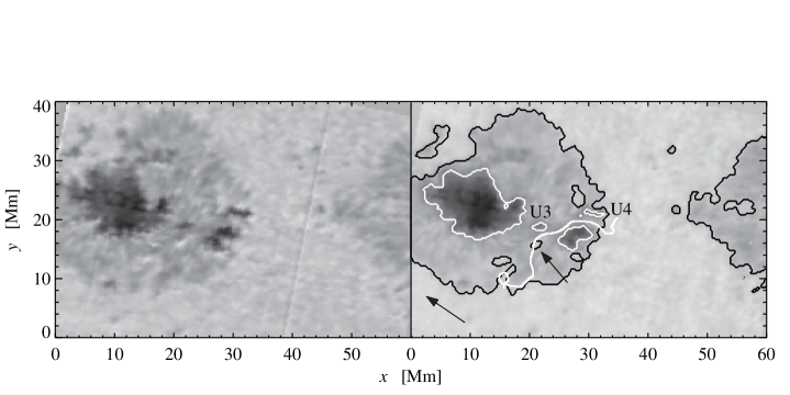
Figure 1.: Slit reconstructed continuum images of the spot near Fe i 1078.3 nm (left), and near Ca ii 854.2 nm (right). The arrow in the lower left corner points to disk center. Contours mark the boundaries of umbra and penumbra. Small umbrae are marked as U3 and U4, and another arrow points to a bright feature close to the PIL (thick white line). The axis orientation corresponds to the solar North and West directions.

The sunspot group NOAA 11504 consisted on 2012, June 17 of three major spots, and one of them harbored smaller umbrae other than the main umbra. Close to the outer boundary but still inside the complex penumbra was an extended dark feature with opposite magnetic polarity with respect to the main umbra. In the following, we call this feature the $\delta$-umbra. The group was located 35^∘ from disk center at 18^∘S/29^∘W (cos $\vartheta$ = 0.82). We observed this sunspot with the Vacuum Tower Telescope (VTT) in Tenerife. The full Stokes vector in two different spectral lines, Fe i 1078.3 nm and Si i 1078.6 nm, was recorded with the Tenerife Infrared Polarimeter (TIP; Collados et al. 2007). As Balthasar & Gömöry (2008) pointed out, these two lines originate from different atmospheric layers except for the cool cores of umbrae. Both lines form a normal Zeeman triplet with a splitting factor $g_{\mathrm{eff}}=1.5$. The spectral dispersion was 2.19 pm, and along the slit, two pixel were binned resulting in an image scale of 0$.\!\!^{\prime\prime}$35 per pixel. During the time period 10:00 – 10:38 UT we scanned the sunspot with 180 steps of 0$.\!\!^{\prime\prime}$36 width corresponding to the slit width. Both spatial step widths correspond roughly to the theoretical resolution of the telescope of 0$.\!\!^{\prime\prime}$39. For each scan position we accumulated ten exposures of 250 ms in each modulation state of TIP. Seeing influences were compensated by the Kiepenheuer Adaptive Optics System (KAOS; von der Lühe et al. 2003; Berkefeld et al. 2010). The same data set was also used by Balthasar et al. (2013b).

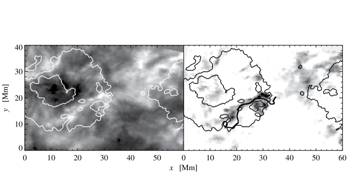
Figure 2.: Line core intensity of the line Ca ii 854.2 nm (left) and negative image of the central emission in this line (right). Contours mark the boundaries of umbra and penumbra as well as the PIL.

The magnetic vector field and the Doppler velocities of these two lines were derived with the Stokes Inversion based on Response functions (SIR). This code was developed by Ruiz Cobo & del Toro Iniesta (1992). We set three nodes for the temperature and kept magnetic field strength $B$, inclination $\gamma$, and azimuth $\psi$ constant with height, as well as the Doppler velocity $v_{\mathrm{D}}$. We obtained the height dependence of these parameters by inverting the two lines separately. We used a single-component model atmosphere. The SIR code provided also error estimates for the calculated quantities, and we processed these errors by error propagation to get the errors of the final physical parameters. The next issue was to solve the magnetic azimuth ambiguity. In the first step, we assumed a single azimuth center in the main umbra and chose that direction which had the smaller difference to the radial orientation. It had to be considered that this orientation is inward because of the negative polarity on the main umbra. This way we obtained a roughly correct start azimuth (although the $\delta$-umbra had its own azimuth center) for the minimum energy method provided by Leka et al. (2009). With this method, the term $|\nabla\cdot\vec{B}|+w|J_{\mathrm{z}}|$ is minimized. $J_{\mathrm{z}}$ is the vertical component of the electric current density and $w$ is a weighting factor. The output delivers a reliable magnetic azimuth. Finally we rotated all images to the local reference frame.

Next to TIP, we mounted a CCD-camera to record spectra of the line Ca ii 854.2 nm and another photospheric line Si i 853.6 nm with a high excitation potential of 6.15 eV, which probes the deep layers of the solar atmosphere (see Beck & Rezai 2012). With this setup, we had a dispersion of 0.82 pm per pixel. This CCD-camera could not be synchronized with TIP. Therefore we integrated over 9 s and used these data only as intensity spectra to determine Doppler velocities and line core intensities of the Ca line. Doppler velocities of the Si line were determined from the minimum position of a parabola fit. Because this line becomes very weak in the cool parts of the umbra, velocities are rather noisy there. For the Ca line, we distinguish between three different cases. If there was no central emission, as usual, we determined the minimum of a polynomial fit of fourth degree. If we detected central emission with a single peak, we applied a parabola fit to this central emission and calculated its maximum position. In some cases, we encountered a central reversal in the emission. In these cases, we fit a polynomial of fourth degree, and its central minimum was used to determine the Doppler velocity. Central emission occurs in the $\delta$-spot along a line dividing the lower right part of the penumbra in Fig. 1. In the following, we call this line the ‘Central Emission Line’ (CEL). The CEL is partly co-spatial with the PIL, but not everywhere. Fig. 2 shows the line core intensities of the infrared Ca line and the maximum intensity of the central emission after subtraction of a parabel fit through the wings of the line.

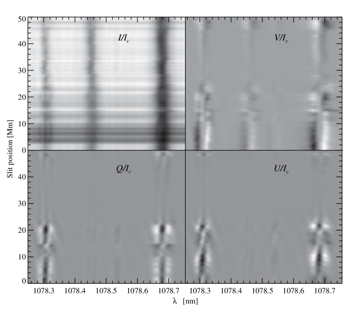
Figure 3.: Maps of the Stokes-profiles $I/I_{c}$, $Q/I_{c}$, $U/I_{c}$, and $V/I_{c}$, normalized to the continuum intensity at disk center $I_{c}$ for a selected slit position. Scalings are: $I/I_{c}$ 0.35–1.0, $V/I_{c}\pm-0.1$, and $Q/I_{c}$ and $U/I_{c}\pm 0.08$. Note the weak multi-lobe $Q/I_{c}$-profiles at 12 Mm along the slit.

All maps were destretched with the method described by Verma et al. (2012) to get quadratic pixels with a side length of 260 km on the Sun.

3 Results

Slit reconstructed intensity maps are shown in Fig. 1. The spot exhibited a complex structure of the penumbra, which harbored several dark features beside the main umbra. Most of them had the same polarity as the main umbra, but the bow-shaped feature in the South-West part of the penumbra was the $\delta$-umbra, i.e., it had the opposite polarity. The $\delta$-umbra had the same polarity as the leading spot of the group, which is partly seen on the right side of Fig. 1. We also see some bright inclusions in the penumbra, and one of them, marked by an arrow in Fig. 1, seems to play a special role in the magnetic configuration. Between main and $\delta$-umbra there was a another small umbra U3, which had the same polarity as the main umbra. Another small umbra U4 close to the $\delta$-umbra also had the polarity of the main umbra.

Maps of the Stokes-profiles at a selected slit position are shown in Fig. 3. Weak multi-lobe $Q$-profiles appear at 12 Mm along the slit.

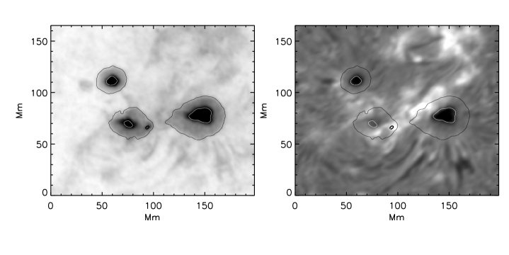
Figure 4.: Images obtained with ChroTel in the core of the He i line at 1083.03 nm (left) and in H$\alpha$ (right). Black and white contours mark penumbra and umbrae, respectively.

Context images in the line cores of H$\alpha$ and the He i line at 1083.03 nm were obtained with the Chromospheric Telescope (ChroTel; Bethge et al. 2011, 2012). On this day, the ChroTel observations started at 10:45 UT, and we used the first images of the series shown in Fig. 4. In the helium image, we see mainly photospheric structures because this line is normally weak compared to H$\alpha$. In H$\alpha$, the umbrae of the two neighboring spots ($x,y\sim$ 60 Mm, 110 Mm and 150 Mm, 75 Mm) are well visible, while it is very hard to identify the umbrae of the $\delta$-spot ($x,y\sim$ 75 Mm, 70 Mm). Here, the photospheric structures were completely covered by chromospheric features indicating that the magnetic field in the chromosphere plays an important role in $\delta$-spots. Especially, we detected a brightening in H$\alpha$ along the CEL. An even stronger brightening occured in the prolongation of the CEL along the outer penumbral boundary of the leading spot of this group.

3.1 Magnetic field

The total magnetic field strength is shown in Fig. 5. In the main umbra we found 2600 G in the Fe i 1078.3 nm line and 2570 G in the Si i 1078.6 nm line, typical for medium sized sunspots. The values in the $\delta$-umbra were 2250 G and 2030 G, respectively. The field strength dropped to 1500 G from the iron line and and 1400 G from the silicon line in the area between main and $\delta$-umbra. Umbral core U3 exhibited 2000 G in the iron line, but only 1500 G in the silicon line.

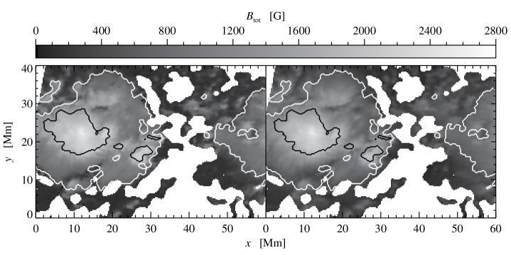
Figure 5.: Total magnetic field strength from Fe i 1078.3 nm (left), and from Si i 1078.6 nm (right). Areas with insignificant polarization outside the spot are white.

The magnetic inclination in Fig. 6 was close to 180^∘ in the main umbra indicating the negative polarity. In and around the $\delta$-umbra, we encountered small inclinations because of the positive polarity here. Between the two umbrae the inclination changed rapidly from about 150^∘ to about 60^∘, and only at the PIL it was horizontal (90^∘). Inside U3 and U4, the field was less inclined than in its surroundings. The magnetic field was also more vertical at the CEL, where it was not cospatial with the PIL.

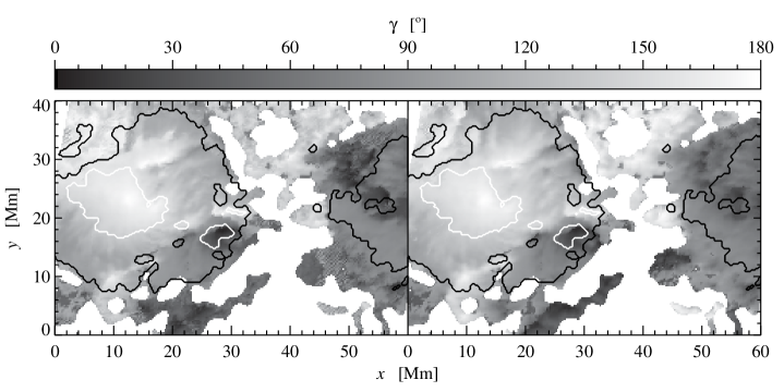
Figure 6.: Inclination of the magnetic field.

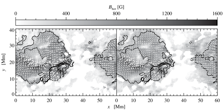
Figure 7.: Horizontal component of the magnetic field. The strength is given by the gray-scale and the azimuth by the white arrows.

The horizontal component of the magnetic field is shown in Fig. 7. We see a smooth transition from the main umbra to the $\delta$-umbra. The strongest horizontal field surrounded the $\delta$-umbra. At some distance to the $\delta$-umbra, close to a small bright feature in the intensity maps, the field lines were almost perpendicular to each other. At this location, the Stokes profiles were anomalous (see Fig. 3), and a single-component inversion was not able to reproduce these profiles. Lites et al. (2002) interpreted such a configuration by an interleaved system of magnetic field lines.

3.2 Height dependence of the magnetic field

Within the framework of our data we have two possibilities to determine the height dependence of the magnetic field. The first option is to take the difference of the magnetic quantities derived from the two lines and divide it by the height difference for the two lines. The height differences were determined in the same way as by Balthasar & Gömöry (2008), who used the depression contribution functions for two different model atmospheres and interpolated according to the local temperature. The results are shown in Fig. 8.

In the main umbra, we found a mean decrease of the total magnetic field strength by 1.9 G km^-1, which is comparable to values published for other spots. The decrease was much steeper in the $\delta$-umbra, here we encountered 5.6 G km^-1. Along the common part of PIL and CEL and in U3 the magnetic field decreased by 3–4 G km^-1, but along the CEL where it was separated from the PIL, the magnetic field strength was increasing by 1 G km^-1. A fast decrease was also observed in U4. Outside the spot, the magnetic field is increasing with height because of the canopy effect. The gradient of the absolute vertical component exhibited a similar behavior. In the $\delta$-umbra, U3, and U4, the decrease was even slightly faster than for the total field strength indicating that the magnetic field became more horizontal above these features. Along the whole CEL, $B_{\mathrm{z}}$ was increasing with height, while the total field strength was decreasing in the common range of CEL and PIL. This discrepancy is explained by a fast decrease of the horizontal magnetic field here. In the mid penumbra, we observed that the vertical component increased with height because the magnetic field was more vertical in higher layers.

The second option is applicable only for the vertical component of the magnetic field and starts from the condition that $\nabla\cdot\vec{B}$ is zero, and vertical partial derivatives must be compensated by the horizontal ones:

$${\partial B_{\mathrm{z}}\over\partial z}=-\left({\partial B_{\mathrm{x}}\over\partial x}+{\partial B_{\mathrm{y}}\over\partial y}\right)$$ (1)

The horizontal derivatives were derived from differences of the values from neighboring pixels, as described by Balthasar (2006).

Qualitatively, the results were similar to those of the difference method, but as Balthasar & Gömöry (2008) and Balthasar et al. (2013a) found, the values were smaller by a factor of about two as shown in Fig 9. The vertical component of the magnetic field decreased faster with height in the $\delta$-umbra, U3 and U4 than in the main umbra. Along the CEL, there was a tendency for an increasing $B_{\mathrm{z}}$ with height.

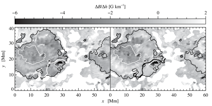
Figure 8.: Height gradients of the total magnetic field $B$ (left) and the absolute value of the vertical component $B_{\mathrm{z}}$ (right) derived from the formation-height difference of the two lines Fe i 1078.3 nm and Si i 1078.6 nm.

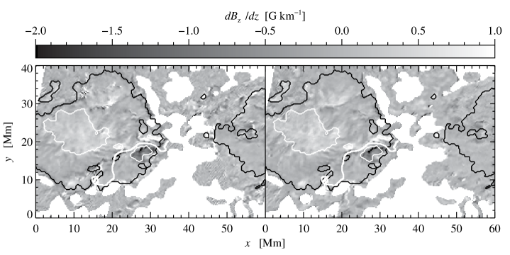
Figure 9.: Height gradients of the vertical component of the the magnetic field derived via $\nabla\cdot\vec{B}=0$ from Fe i 1078.3 nm (left) and from Si i 1078.6 nm (right).

3.3 Electric current densities

The horizontal partial derivatives of the magnetic field also allow us to determine the vertical component of electric current densities $J_{\mathrm{z}}$ according to

$$J_{\mathrm{z}}={1\over\mu}(\nabla\times\vec{B})_{\mathrm{z}}={1\over\mu}\left({\partial B_{\mathrm{y}}\over\partial x}-{\partial B_{\mathrm{x}}\over\partial y}\right),$$ (2)

where $\mu$ is the magnetic permeability. Partial derivatives were estimated from differences between neighboring pixels. This procedure was used before by Balthasar (2006). The results are shown in Fig. 10. Positive current densities of more than 200 mA m^-2 occurred near the outer boundary inside the $\delta$-umbra along a line parallel to the PIL. The maximum value from the iron line is 273 $\pm$ 76 mA m^-2. Along the CEL, we detected negative current densities. Close to the $\delta$-umbra the negative current densities might be a counterpart to the positive values inside the $\delta$-umbra. Negative current densities were still found in the part of the CEL, where it was separated from the PIL. Strong current densities are much more pronounced in the Fe i 1078.3 nm line than in the Si i 1078.6 nm line, i.e., the currents occurred mainly in deep atmospheric layers.

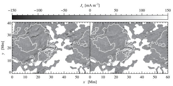
Figure 10.: Vertical component of electric current densities from Fe i 1078.3 nm (left) and Si i 1078.6 nm (right). Values are clipped at $\pm$150 mA m^-2.

3.4 Doppler velocities and proper motions

The Doppler velocities were investigated by Balthasar et al. (2013b). The dominant feature in the photosphere was the Evershed-effect which was interrupted at the CEL. A special feature is a blueshift at the PIL which Balthasar et al. (2013b) interpreted as Evershed-effect related to the $\delta$-umbra. In the chromosphere above the CEL, small locations exhibited downflows up to 8 km s^-1, derived from the line Ca ii 854.2 nm. One of these downflow patches was very close to the bright feature marked in Fig. 1. Another downflow patch is located just outside the penumbra, similar as a patch observed by Balthasar et al. (2013a) near a single sunspot. Other locations along the CEL exhibited upflows of the same order of magnitude as the downflows.

Proper motions also were investigated by Balthasar et al. (2013b). They used a time series of magnetograms from the Helioseismic and Magnetic Imager (HMI, Schou et al. 2012) on board of the Solar Dynamic Observatory (SDO, Pesnell et al. 2012) and applied the Differential Affine Velocity Estimator (DAVE) developed by Schuck (2005, 2006). This method delivered ‘magnetic flux transfer velocities’ (Schuck 2006), that do not necessarily represent plasma flows. The flux transfer velocities pointed towards the $\delta$-umbra, where its Evershed effect was visible as blue-shift. A flow of 0.25 km s^-1 away from the $\delta$-umbra parallel to the CEL was detected, which crossed the PIL, where it was separated from the CEL. On the other side of the CEL, towards the main umbra, only 0.05 km s^-1 were found, resulting in a shear imbalance of 0.2 km s^-1. A counterclockwise spiral motion covered a part of the $\delta$-umbra and U4, but we did not detect that the whole $\delta$-umbra was rotating.

4 Discussion

The discrepancy between different methods to derive the height gradient of the vertical component of the magnetic field strength is a long-lasting problem in solar physics and has been discussed by Leka & Metcalf (2003), Balthasar & Gömöry (2008), and Balthasar et al. (2013a). Determining geometrical heights from contribution or response functions has uncertainties, and one has to keep in mind that such functions cover an extended height range. Height gradients determined by this method but from different lines have similar values around 2 G km^-1 (see Wittmann 1974; Balthasar & Schmidt 1993; Moran et al. 2000; Leka & Metcalf 2003). To solve the problem with larger differences of the line formation, one would need to extend the solar atmosphere to much more than a few hundred kilometers. Similar gradients were also derived from height-dependent inversions as carried out by Westendorp Plaza et al. (2001), Mathew et al. (2003), and Sánchez Cuberes et al. (2005). However, comparing with a coronal C iv line at 154.8 nm, Hagyard et al. (1983) obtained gradients of 0.1–0.2 G km^-1. Using $\nabla\cdot\vec{B}$, Hofmann & Rendtel (1989) obtained 0.32 G km^-1 from data with low spatial resolution. Many solar structures are rather small, i.e., at the spatial resolution limit of present instruments or even below. Thus, features that do not belong to the same magnetic structure enter the determination of the horizontal gradients and affect the vertical gradients. Indications where found by Balthasar et al. (2013a) that higher spatial resolution decreases this discrepancy. So far, the problem is not solved, but independent from the solution of this problem, we can state that the magnetic field decreases much faster with height above the $\delta$-umbra than above the main umbra.

The CEL might be the dividing line between the original spot and new emerging flux forming the $\delta$-umbra. The penumbral area between PIL and CEL then would be the following part of the new bipolar flux. Penumbrae merged between main and $\delta$-umbra, i.e., between opposite polarities, similar as observed by Wang et al. (2013), but not for the parts with the same polarity. This scenario explains that the Evershed flow belonging to the main umbra ended at the CEL. The horizontal flux transfer velocities were parallel to the CEL and did not cross it, in contrast to the PIL. Strong changes of the magnetic field with height in this area are not surprising, and there were electric currents at the CEL. Such an emerging flux system would also explain that the CEL representing the dividing line between old and new flux is more important for the configuration of this $\delta$-spot than the PIL.

The observed chromospheric downflows above the CEL resemble the supersonic downflows found by Martínez Pillet et al. (1994) at the PIL of another sunspot, but in the photosphere. We could not detect such large vertical velocities in the photosphere. Perhaps, the photospheric counterparts to the chromospheric flows were rather narrow, much less than the 2^′′ in case of Martínez Pillet et al. (1994), and they contributed only a small fraction of the signal in our resolution element.

The group NOAA 11504 produced a C1.8 flare about 19 hours before our observations and a C3.9 flare seven hours after our observations as shown in Fig. 11. We did not find a shear flow in this group next to the $\delta$-umbra. The flow away from it parallel to the CEL is probably not strong enough to build up magnetic shear within a short period. This indicates that a $\delta$-spot can be quiet in the sense of flares for at least a day.

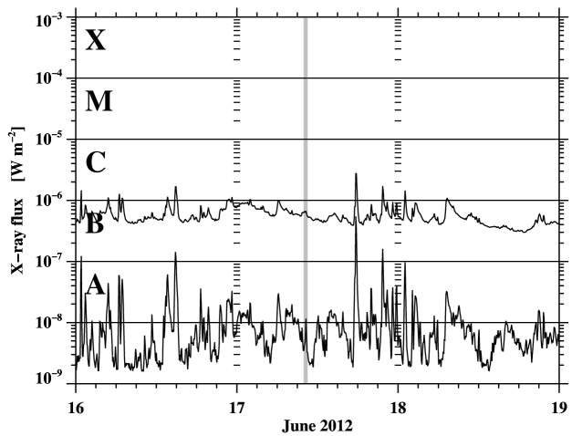
Figure 11.: X-ray flux in the 1.0–8.0 Å (top) and 0.5–4.0 Å (bottom) channels of the of the GOES-satellite for the period 2012, June 16–18. The gray vertical bar marks our VTT-observing time. For an easier readability, logarithmic scale marks are repeated at the beginning of each day.

5 Conclusions

In the following, we summarize the most important findings with regard to this $\delta$-spot in NOAA 11504.

$\bullet$

The magnetic field strength of 2250 G in the $\delta$-umbra is somewhat less than in the main umbra (2600 G in deep photospheric layers).

$\bullet$

We find that the magnetic field transition between the main and the $\delta$-umbra is rather smooth. A small location, where the magnetic azimuth changes by about 90^∘ from one pixel to the next, occurrs at some distance from the $\delta$-umbra close to a bright patch next to the PIL.

$\bullet$

The magnetic field decreases much faster with height above the $\delta$-umbra than above the main umbra.

$\bullet$

Electric currents are detected at the CEL in deep photospheric layers and in the $\delta$-umbra.

$\bullet$

Around the main umbra, we observe the typical Evershed flow which ends in the southeastern part of the spot at the CEL.

$\bullet$

Related to the $\delta$-umbra, we detect a second system of Evershed flows.

$\bullet$

Large velocities of $\pm$8 km s^-1 occur in the chromosphere above the CEL.

$\bullet$

No major flare was observed within seven hours before or after our observations.

We have shown that the CEL is more important than the PIL for this specific sunspot. We are able to explain this assuming that the CEL is the dividing line between old and new emerging bipolar flux. Thus, $\delta$-spots can be stable, they do not always produce flares. The brightenings in H$\alpha$ and the occurrence of central emission in the Ca ii 854.2 nm line must be explained by physical processes related to the magnetic field in the chromosphere, and these processes play an important role for the configuration of this $\delta$-spot. Future observations should include also measurements of the chromospheric magnetic field. This will be possible with, e.g., with the GREGOR Infrared Spectrograph (Collados et al. 2012) or the GREGOR Fabry Pérot Interferometer (Puschmann et al. 2012) at the new GREGOR solar telescope (Schmidt et al. 2012) in Tenerife.

Acknowledgments

The VTT and ChroTel are operated by the Kiepenheuer-Institut für Sonnenphysik (Germany) at the Spanish Observatorio del Teide of the Instituto de Astrofísica de Canarias. The HMI-data have been used by courtesy of NASA/SDO and the HMI science team. MV expresses her gratitude for the generous financial support by the German Academic Exchange Service (DAAD) in the form of a Ph.D. scholarship. CD and REL were supported by grant DE 787/3-1 of the German Science Foundation (DFG).

References

- Balthasar (2006) Balthasar, H. 2006, A&A, 449, 1169
- Balthasar et al. (2013a) Balthasar, H., Beck, C., Gömöry, P., Muglach, K., Puschmann, K. G., Shimizu, T., & Verma, M. 2013a, Central European Astrophysical Bulletin, 37, 435
- Balthasar et al. (2013b) Balthasar, H., Beck, C., Louis, R. E., Verma, M., & Denker, C. 2013b, A&A, xxx, (submitted)
- Balthasar & Gömöry (2008) Balthasar, H., & Gömöry, P. 2008, A&A, 488, 1085
- Balthasar & Schmidt (1993) Balthasar, H., & Schmidt, W. 1993, A&A, 279, 243
- Beck & Rezai (2012) Beck, C., & Rezai, R. 2012, in Second ATST-EAST Meeting: Magnetic Fields from the Photosphere to the Corona, edited by T. R. Rimmele, A. Tritschler, F. Wöger, M. Collados Vera, H. Socas-Navarro, R. Schlichenmaier, M. Carlsson, T. Berger, A. Cadavid, P. R. Gilbert, P. R. Goode, & M. Knölker (San Francisco), vol. 463 of Astronomical Society of the Pacific Conference Series, 257
- Berkefeld et al. (2010) Berkefeld, T., Soltau, D., Schmidt, D., & von der Lühe, O. 2010, Appl. Opt., 49, G155
- Bethge et al. (2012) Bethge, C., Beck, C., Peter, H., & Lagg, A. 2012, A&A, 537, A130
- Bethge et al. (2011) Bethge, C., Peter, H., Kentischer, T., Halbgewachs, C., Elmore, D. F., & Beck, C. 2011, A&A, 534, A105
- Collados et al. (2007) Collados, M., Lagg, A., Díaz García, J. J., Hernández Suárez, E., López López, R., Páez Maña, E., & Solanki, S. K. 2007, in The Physics of Chromospheric Plasmas, edited by P. Heinzel, I. Dorotovič, & R. J. Rutten (San Francisco), vol. 368 of Astronomical Society of the Pacific Conference Series, 611
- Collados et al. (2012) Collados, M., López, R., Páez, E., Hernández, E., Reyes, M., Calcines, A., Ballesteros, E., Díaz, J. J., Denker, C., Lagg, A., & et al. 2012, AN, 333, 872
- Denker et al. (2007) Denker, C., Deng, N., Tritschler, A., & Yurshyshyn, V. 2007, Sol. Phys, 245, 219
- Fischer et al. (2012) Fischer, C. E., Keller, C. U., Snik, F., Fletcher, L., & Socas-Navarro, H. 2012, A&A, 547, A34
- Hagyard et al. (1983) Hagyard, M. J., Teuber, D., West, E. A., Tandberg-Hanssen, E., Henze, W. J., Beckers, J. M., Bruner, M., Hyder, C. L., & Woodgate, B. E. 1983, Sol. Phys., 84, 13
- Hofmann & Rendtel (1989) Hofmann, A., & Rendtel, J. 1989, AN, 310, 61
- Jennings et al. (2002) Jennings, D. E., Deming, D., McCabe, G., Sada, P. V., & Moran, T. 2002, ApJ, 568, 1043
- Künzel (1960) Künzel, H. 1960, AN, 285, 271
- Künzel (1964) — 1964, AN, 288, 177
- Leka et al. (2009) Leka, K. D., Barnes, G., Crouch, A. D., Metcalf, T. R., Gary, G. A., Jing, J., & Liu, Y. 2009, Sol. Phys., 260, 83
- Leka & Metcalf (2003) Leka, K. D., & Metcalf, T. R. 2003, Sol. Phys., 212, 361
- Lites et al. (2002) Lites, B. W., Socas-Navarro, H., & Skumanich, A. 2002, ApJ, 575, 1131
- Martínez Pillet et al. (1994) Martínez Pillet, V., Lites, B. W., Skumanich, A., & Degenhardt, D. 1994, ApJ, 425, L113
- Mathew et al. (2003) Mathew, S. K., , Lagg, A., Solanki, S. K., Collados, M., Borrero, J. M., Berdyugina, S., Krupp, N., Woch, J., & Frutiger, C. 2003, A&A, 410, 695
- Min & Chae (2009) Min, S., & Chae, J. 2009, Sol. Phys., 258, 203
- Moran et al. (2000) Moran, T., Deming, D., Jennings, D. E., & McCabe, G. 2000, ApJ, 533, 1035
- Pesnell et al. (2012) Pesnell, W. D., Thompson, B. J., & Chamberlin, P. C. 2012, Sol. Phys., 275, 3
- Puschmann et al. (2012) Puschmann, K. G., Denker, C., Kneer, F., Al Erdogan, N., Balthasar, H., Bauer, S. M., Beck, C., Bello González, N., Collados, M., Hahn, T., & et al. 2012, AN, 333, 880
- Ruiz Cobo & del Toro Iniesta (1992) Ruiz Cobo, B., & del Toro Iniesta, J. C. 1992, ApJ, 398, 275
- Sammis et al. (2000) Sammis, I., Tang, F., & Zirin, H. 2000, ApJ, 540, 583
- Sánchez Cuberes et al. (2005) Sánchez Cuberes, M., Puschmann, K. G., & Wiehr, E. 2005, A&A, 440, 345
- Schmidt et al. (2012) Schmidt, W., von der Lühe, O., Volkmer, R., Denker, C., Solanki, S. K., Balthasar, H., Bello González, N., Berkefeld, T., Collados, M., Fischer, A., & et al. 2012, AN, 333, 796
- Schou et al. (2012) Schou, J., Scherrer, P. H., Bush, R. I., Wachter, R., Couvidat, S., Rabello-Soares, M. C., Bogart, R. S., Hoeksema, J. T., Liu, Y., Duvall, T. L., & et al. 2012, Sol. Phys., 275, 229
- Schuck (2005) Schuck, P. W. 2005, ApJ, 632, L53
- Schuck (2006) — 2006, ApJ, 646, 1358
- Takizawa et al. (2012) Takizawa, K., Kitai, R., & Zhang, Y. 2012, Sol. Phys., 281, 599
- Tan et al. (2009) Tan, C., Chen, P. F., Abramenko, V., & Wang, H. 2009, ApJ, 690, 1820
- Török et al. (2013) Török, T., Temmer, M., Valori, G., Veronig, A. M., van Driel-Gestelyi, L., & Vršnak, B. 2013, Sol. Phys., 286, 453
- Verma et al. (2012) Verma, M., Balthasar, H., Deng, N., Liu, C., Shimizu, T., Wang, H., & Denker, C. 2012, A&A, 538, A109
- von der Lühe et al. (2003) von der Lühe, O., Soltau, D., Berkefeld, T., & Schelenz, T. 2003, in Innovative Telescopes and Instrumentation for Solar Astrophysics, edited by S. L. Keil, & S. V. Avakyan (Washington D.C.), vol. 4853 of Proceedings of the SPIE, 187
- Wang et al. (2013) Wang, H., Liu, C., Wang, S., Deng, N., Xu, Y., Jing, J., & Cao, W. 2013, ApJ, 774, L24
- Westendorp Plaza et al. (2001) Westendorp Plaza, C., del Toro Iniesta, J. C., Ruiz Cobo, B., Martínez Pillet, V., Lites, B. W., & Skumanich, A. 2001, ApJ, 547, 1130
- Wittmann (1974) Wittmann, A. 1974, Sol. Phys., 36, 29