Mass distributions marginalized over per-event errors

D. Martínez Santos F. Dupertuis NIKHEF and VU University Amsterdam, Amsterdam, The Netherlands Ecole Polytechnique Fédérale de Lausanne (EPFL), Lausanne, Switzerland
Abstract

We present generalizations of the Crystal Ball function to describe mass peaks in which the per-event mass resolution is unknown and marginalized over. The presented probability density functions are tested using a series of toy MC samples generated with Pythia and smeared with different amounts of multiple scattering and for different detector resolutions.

keywords:
statistics , invariant mass peaks
journal: Nuclear Instruments and Methods

1 Introduction

A very common probability density function (p.d.f.formulae-sequence𝑝𝑑𝑓p.d.f.) used to fit the mass peak of a resonance in experimental particle physics is the so-called Crystal Ball (CB) function [1, 2, 3]:

p(m){e12(mμσ)2, if mμσ>aA(Bmμσ)n, otherwiseproportional-to𝑝𝑚casessuperscript𝑒12superscript𝑚𝜇𝜎2, if 𝑚𝜇𝜎𝑎𝐴superscript𝐵𝑚𝜇𝜎𝑛, otherwisep(m)\propto\begin{cases}e^{-\frac{1}{2}\left(\frac{m-\mu}{\sigma}\right)^{2}}&\text{, if }\frac{m-\mu}{\sigma}>-a\\ A\left(B-\frac{m-\mu}{\sigma}\right)^{n}&\text{, otherwise}\end{cases} (1)

where m𝑚m is the free variable (the measured mass), μ𝜇\mu is the most probable value (the resonance mass), σ𝜎\sigma the resolution, a𝑎a is called the transition point and n𝑛n the power-law exponent. A𝐴A and B𝐵B are calculated by imposing the continuity of the function and its derivative at the transition point a𝑎a. This function consists of a Gaussian core, that models the detector resolution, with a tail on the left-hand side that parametrizes the effect of photon radiation by the final state particles in the decay. In data analysis, one may deal with events which have different uncertainties on the measured mass, therefore distorting the core of the Crystal Ball, which will not be a Gaussian any more. This is sometimes modelled by the sum of two or three Crystal Ball functions, which is the equivalent of assuming that the per-event uncertainty is a sum of two or three delta functions. However, per-event uncertainties are usually continuous functions very different from a sum of a small number of deltas. One way of dealing with per-event uncertainties that follow a certain distribution, is to either make a p.d.f.formulae-sequence𝑝𝑑𝑓p.d.f. conditional on the per-event uncertainty (if its distribution is known) or to perform the analysis in bins of the quantities that affect the per-event uncertainties (for example, particle momenta) and combine them afterwards. However, those procedures can significantly complicate the analysis, and in some cases one may prefer to simply marginalize over the mass error and have a p.d.f.formulae-sequence𝑝𝑑𝑓p.d.f. that describes the final mass peak, as:

p(m)01ve12v(mμ)2ρ(v)𝑑vproportional-to𝑝𝑚superscriptsubscript01𝑣superscript𝑒12𝑣superscript𝑚𝜇2𝜌𝑣differential-d𝑣p(m)\propto\int_{0}^{\infty}\frac{1}{\sqrt{v}}e^{-\frac{1}{2v}(m-\mu)^{2}}\rho(v)dv (2)

where v𝑣v is the variance and ρ(v)𝜌𝑣\rho(v) the prior density of the variance.

In this paper, we will define some extensions of the Crystal Ball distribution for different assumptions on ρ(v)𝜌𝑣\rho(v). We will fit the proposed mass models to J/ψμ+μ𝐽𝜓superscript𝜇superscript𝜇J/\psi\to\mu^{+}\mu^{-} toy MC samples where we can modify the relative importance of multiple scattering (MS) and detector spatial resolution (hereafter SR). Section 2 describes the generation of the toy MC samples. Section 3 defines an extension of the CB using a hyperbolic distribution core. Sections 4 and 5 generalize the function defined in Sect. 3. Section 6 gives a brief discussion of the meaning of the fit parameters. Section 7 discusses other effects on the invariant mass line-shape that are not directly related to resolution. Conclusions are drawn in Sect. 8.

2 Simulation of J/ψμ+μ𝐽𝜓superscript𝜇superscript𝜇J/\psi\to\mu^{+}\mu^{-} decays

We generate J/ψ𝐽𝜓J/\psi events at s=𝑠absent\sqrt{s}= 8 TeV using the main17.cc script of Pythia8.176 [4]. The J/ψ𝐽𝜓J/\psi’s are then isotropically decayed into two muons. No photons are added, as the radiative tail of the mass distribution should be well accounted by the Crystal Ball tail.

The generated muon momenta are smeared with a Gaussian resolution which has a momentum dependence:

σ(p)p=a+bp𝜎𝑝𝑝𝑎𝑏𝑝\frac{\sigma(p)}{p}=a+bp (3)

where a𝑎a mimics the multiple scattering (MS) and b𝑏b mimics the effect of the hit resolution. We take as typical values a=3×10³𝑎3superscript103a=3\times 10^{-3} and b=2×10⁵GeV1c𝑏2superscript105superscriptGeV1𝑐b=2\times 10^{-5}\ \mathrm{GeV}^{-1}c inspired by [5], although we will vary them for different tests.

3 Hyperbolic resolution model

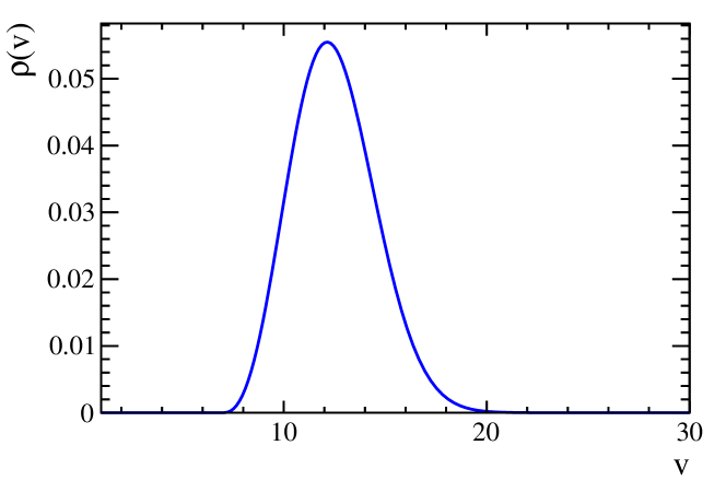
A very flexible function that describes asymmetric unimodal p.d.f.formulae-sequence𝑝𝑑𝑓p.d.f.’s defined above a certain threshold (i.e, like per-event error distributions usually look like, see for example Fig. 6 in [6]) is the so-called Amoroso distribution [7] (see Fig. 1). If we consider the Amoroso distribution as a potential implementation for ρ(v)𝜌𝑣\rho(v), then the corresponding core of the invariant mass p.d.f.formulae-sequence𝑝𝑑𝑓p.d.f. will be the following:

Φ(m)01ve12v(mμ)2(vv0θ)αβ1e(vv0θ)β𝑑vproportional-toΦ𝑚superscriptsubscript01𝑣superscript𝑒12𝑣superscript𝑚𝜇2superscript𝑣subscript𝑣0𝜃𝛼𝛽1superscript𝑒superscript𝑣subscript𝑣0𝜃𝛽differential-d𝑣\Phi(m)\propto\int_{0}^{\infty}\frac{1}{\sqrt{v}}e^{-\frac{1}{2v}(m-\mu)^{2}}\left(\frac{v-v_{0}}{\theta}\right)^{\alpha\beta-1}e^{-\left(\frac{v-v_{0}}{\theta}\right)^{\beta}}dv (4)
Refer to caption
Figure 1: Example of the Amoroso distribution for a hypothetical variance v𝑣v. The parameters used are θ=5𝜃5\theta=5, α=1.5𝛼1.5\alpha=1.5 μ=7𝜇7\mu=7, and β=2.3𝛽2.3\beta=2.3.

Unfortunately, the above integral cannot be solved analytically. It would require a numerical implementation of the core and its derivative. This would make the matching with the radiative tail difficult. Evaluating (4) numerically for different values of Amoroso parameters, we find log-densities that exhibit an hyperbolic profile. Based on that observation, we define a possible core:

c(x)eb1+(mμ)2/δ2proportional-to𝑐𝑥superscript𝑒𝑏1superscript𝑚𝜇2superscript𝛿2c(x)\propto e^{-b\sqrt{1+(m-\mu)^{2}/\delta^{2}}} (5)

i.e, c(x)𝑐𝑥c(x) is the symmetric limit of the hyperbolic distribution. It can also be rewritten in such way that the mass resolution σ𝜎\sigma appears explicitly, as it will be discussed in Sect. 4. Adding a CB-like tail to (5), we obtain the following p.d.f.formulae-sequence𝑝𝑑𝑓p.d.f.:

A(m,μ,b,δ,a,n){eb1+(mμ)2/δ2, if mμδaeb1+a2(n1+a2ba(n1+a2/(ba)a(mμ)/δ))n, otherwiseproportional-to𝐴𝑚𝜇𝑏𝛿𝑎𝑛casessuperscript𝑒𝑏1superscript𝑚𝜇2superscript𝛿2, if 𝑚𝜇𝛿𝑎superscript𝑒𝑏1superscript𝑎2superscript𝑛1superscript𝑎2𝑏𝑎𝑛1superscript𝑎2𝑏𝑎𝑎𝑚𝜇𝛿𝑛, otherwiseA(m,\mu,b,\delta,a,n)\propto\begin{cases}e^{-b\sqrt{1+(m-\mu)^{2}/\delta^{2}}}&\text{, if }\frac{m-\mu}{\delta}\geq-a\\ e^{-b\sqrt{1+a^{2}}}\left(\frac{n\sqrt{1+a^{2}}}{ba(n\sqrt{1+a^{2}}/(ba)-a-(m-\mu)/\delta)}\right)^{n}&\text{, otherwise}\end{cases} (6)

hereafter referred to as the Apollonios distribution, currently being used for cross-checks in data analysis of the LHCb experiment. The core (5) can be obtained analytically for a variance prior density:

ρ(v,b,δ)e(b2v/δ2+δ2/v)proportional-to𝜌𝑣𝑏𝛿superscript𝑒superscript𝑏2𝑣superscript𝛿2superscript𝛿2𝑣\rho(v,b,\delta)\propto e^{-(b^{2}v/\delta^{2}+\delta^{2}/v)} (7)

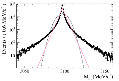
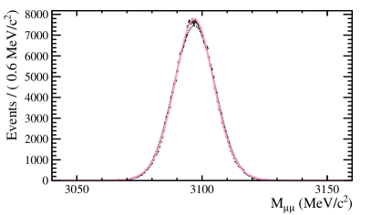
We fit the mass peak for J/ψμ+μ𝐽𝜓superscript𝜇superscript𝜇J/\psi\to\mu^{+}\mu^{-} decays satisfying pTJ/ψ[0,14]GeV/csuperscriptsubscript𝑝𝑇𝐽𝜓014GeV𝑐p_{T}^{J/\psi}\in[0,14]\,{\rm GeV}/c, θμ[20,300]superscript𝜃𝜇20300\theta^{\mu}\in[20,300] mrad, pμ>6GeV/csuperscript𝑝𝜇6GeV𝑐p^{\mu}>6\,{\rm GeV}/c, pTμ>0.5GeV/csuperscriptsubscript𝑝𝑇𝜇0.5GeV𝑐p_{T}^{\mu}>0.5\,{\rm GeV}/c (which mimics LHCb-like conditions) to the Apollonios distribution, and find a very good agreement as can be seen in Fig. 2.

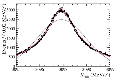
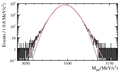
Now, the good agreement between this model and the MC toys used for testing can be broken without too much effort. For example, we now repeat the exercise releasing all kinematic and acceptance cuts, and switching off the MS term. These changes modify the distribution and fit results are shown in Fig. 3, where we see that (5) cannot fit the generated data. However, it is also interesting to note that, even in this extreme case, (5) can do a good job in a region of about two standard deviations around the peak.
Refer to caption
Refer to caption
Figure 2: Fit of the invariant mass distribution of a J/ψμ+μ𝐽𝜓superscript𝜇superscript𝜇J/\psi\to\mu^{+}\mu^{-} generated sample with pTJ/ψ[0,14]superscriptsubscript𝑝𝑇𝐽𝜓014p_{T}^{J/\psi}\in[0,14]GeV/cGeV𝑐\,{\rm GeV}/c, θμ[20,300]subscript𝜃𝜇20300\theta_{\mu}\in[20,300] mrad, pμ>6superscript𝑝𝜇6p^{\mu}>6 GeV/cGeV𝑐\,{\rm GeV}/c and pTμ>0.5superscriptsubscript𝑝𝑇𝜇0.5p_{T}^{\mu}>0.5GeV/cGeV𝑐\,{\rm GeV}/c. The pink line corresponds to the fit to a hyperbolic distribution. The dashed black line corresponds to the fit to a Gaussian. Left: linear scale. Right: Logarithmic scale.
Refer to caption
Refer to caption
Figure 3: Fit of the invariant mass distribution of a J/ψμ+μ𝐽𝜓superscript𝜇superscript𝜇J/\psi\to\mu^{+}\mu^{-} generated sample without any phase space restriction and without the multiple scattering term in the momentum resolution. The pink line corresponds to the fit to an hyperbolic distribution. The dashed black line corresponds to the fit to a Gaussian. Left: Fit in the full mass range. Right: Fit in a region of about two standard deviations around the mean.

4 Generalized Hyperbolic resolution model

The core of (5) is a limit case of the generalized hyperbolic distribution [8]:

G(m,μ,λ,α,β,δ)=((mμ)2+δ2)12λ14eβ(mμ)Kλ12(α(mμ)2+δ2)𝐺𝑚𝜇𝜆𝛼𝛽𝛿superscriptsuperscript𝑚𝜇2superscript𝛿212𝜆14superscript𝑒𝛽𝑚𝜇subscript𝐾𝜆12𝛼superscript𝑚𝜇2superscript𝛿2G(m,\mu,\lambda,\alpha,\beta,\delta)=\left((m-\mu)^{2}+\delta^{2}\right)^{\frac{1}{2}\lambda-\frac{1}{4}}e^{\beta(m-\mu)}K_{\lambda-\frac{1}{2}}\left(\alpha\sqrt{(m-\mu)^{2}+\delta^{2}}\right) (8)

where Kλsubscript𝐾𝜆K_{\lambda} are the cylindrical harmonics or special Bessel functions of third kind. In principle, β2superscript𝛽2\beta^{2} is constrained to be smaller than α2superscript𝛼2\alpha^{2}. In practice that condition can be ignored if the fitting range is finite, but one has to be careful that if β2>α2superscript𝛽2superscript𝛼2\beta^{2}>\alpha^{2} one of the tails will start rising at some point. The generalized hyperbolic distribution also has an important limit case, the Student’s-t distribution, as indicated in Table 1.

Table 1: Limit cases of the generalized hyperbolic distribution
Distributions G(m,μ,λ,α,β,δ)𝐺𝑚𝜇𝜆𝛼𝛽𝛿G(m,\mu,\lambda,\alpha,\beta,\delta)
Hyperbolic λ=1,αδ=bformulae-sequence𝜆1𝛼𝛿𝑏\lambda=1,\alpha\delta=b
Symmetric hyperbolic λ=1,β=0,αδ=bformulae-sequence𝜆1formulae-sequence𝛽0𝛼𝛿𝑏\lambda=1,\beta=0,\alpha\delta=b
Student’s t λ=ν2,α=0,β=0,δ=νformulae-sequence𝜆𝜈2formulae-sequence𝛼0formulae-sequence𝛽0𝛿𝜈\lambda=-\frac{\nu}{2},\alpha=0,\beta=0,\delta=\sqrt{\nu}
Non-standardized Student’s t λ=ν2,α=0,β=0formulae-sequence𝜆𝜈2formulae-sequence𝛼0𝛽0\lambda=-\frac{\nu}{2},\alpha=0,\beta=0

The p.d.f.formulae-sequence𝑝𝑑𝑓p.d.f. in (8) can also be obtained by marginalizing over a variance density111The parameter β𝛽\beta is related to a variance-dependency of the Gaussian mean, and not to the per event variance distribution. For the purpose of this paper β𝛽\beta can be considered zero.:

ρ(v,λ,α,δ)vλ1e[α2v+δ2/v]proportional-to𝜌𝑣𝜆𝛼𝛿superscript𝑣𝜆1superscript𝑒delimited-[]superscript𝛼2𝑣superscript𝛿2𝑣\rho(v,\lambda,\alpha,\delta)\propto v^{\lambda-1}e^{-[\alpha^{2}v+\delta^{2}/v]} (9)

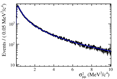
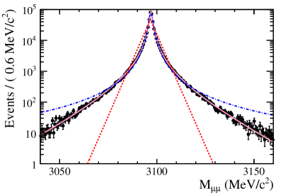
The distribution (9) is the generalized inverse Gaussian distribution and describes very well the density we find for σμμ2superscriptsubscript𝜎𝜇𝜇2\sigma_{\mu\mu}^{2}, for the example in Fig. 3. This is shown in Fig. 5, together with the good agreement between the simulated data and the generalized hyperbolic distribution. We find that (9) fits well the mass variance distribution for all the generated J/ψμ+μ𝐽𝜓superscript𝜇superscript𝜇J/\psi\to\mu^{+}\mu^{-} samples that we have tested, although one needs to add an overall offset to the per-event error, i.e, to change v𝑣v by vv0𝑣subscript𝑣0v-v_{0} in (9). The effect of an overall displacement of the per-event error distribution is further discussed in Sect. 5.

The following re-parametrization {α;δ}{σ;ζ}𝛼𝛿𝜎𝜁\{\alpha;\delta\}\to\{\sigma;\zeta\}:

ζ𝜁\displaystyle\zeta =αδabsent𝛼𝛿\displaystyle=\alpha\delta (10)
σ2superscript𝜎2\displaystyle\sigma^{2} =δ2Kλ+1(ζ)ζKλ(ζ)=δ2Aλ2(ζ)absentsuperscript𝛿2subscript𝐾𝜆1𝜁𝜁subscript𝐾𝜆𝜁superscript𝛿2subscriptsuperscript𝐴2𝜆𝜁\displaystyle=\delta^{2}\frac{K_{\lambda+1}(\zeta)}{\zeta K_{\lambda}(\zeta)}=\delta^{2}A^{-2}_{\lambda}(\zeta) (11)

is more suitable for fitting purposes as it allows us to specify the rms (σ𝜎\sigma) of the distribution in the symmetric case (β=0𝛽0\beta=0) as an explicit parameter. Aλ2=ζKλ(ζ)Kλ+1(ζ)subscriptsuperscript𝐴2𝜆𝜁subscript𝐾𝜆𝜁subscript𝐾𝜆1𝜁A^{2}_{\lambda}=\frac{\zeta K_{\lambda}(\zeta)}{K_{\lambda+1}(\zeta)} is introduced for further convenience. In that parametrization:

G(m,μ,σ,λ,ζ,β)((mμ)2+Aλ2(ζ)σ2)12λ14eβ(mμ)Kλ12(ζ1+(mμAλ(ζ)σ)2)proportional-to𝐺𝑚𝜇𝜎𝜆𝜁𝛽superscriptsuperscript𝑚𝜇2subscriptsuperscript𝐴2𝜆𝜁superscript𝜎212𝜆14superscript𝑒𝛽𝑚𝜇subscript𝐾𝜆12𝜁1superscript𝑚𝜇subscript𝐴𝜆𝜁𝜎2G(m,\mu,\sigma,\lambda,\zeta,\beta)\propto\\ \left((m-\mu)^{2}+A^{2}_{\lambda}(\zeta)\sigma^{2}\right)^{\frac{1}{2}\lambda-\frac{1}{4}}e^{\beta(m-\mu)}K_{\lambda-\frac{1}{2}}\left(\zeta\sqrt{1+(\frac{m-\mu}{A_{\lambda}(\zeta)\sigma})^{2}}\right) (12)

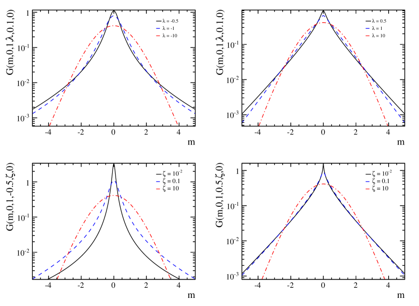
Figure 4 shows G(m,μ,σ,λ,ζ,β)𝐺𝑚𝜇𝜎𝜆𝜁𝛽G(m,\mu,\sigma,\lambda,\zeta,\beta) for different values of ζ𝜁\zeta and λ𝜆\lambda.

Refer to caption
Figure 4: G(m,μ,σ,λ,ζ,β)𝐺𝑚𝜇𝜎𝜆𝜁𝛽G(m,\mu,\sigma,\lambda,\zeta,\beta) is plotted for standard values of μ𝜇\mu, σ𝜎\sigma, β𝛽\beta and different values of ζ𝜁\zeta and λ𝜆\lambda. Top: ζ𝜁\zeta is fixed to 0.1 and λ𝜆\lambda is varied. Bottom: λ𝜆\lambda is fixed to -0.5 for the left plot and 0.5 for the right plot and ζ𝜁\zeta is varied.

Using (12) as the core of a CB-like function, we define:

I(m,μ,σ,λ,ζ,β,a,n){((mμ)2+Aλ2(ζ)σ2)12λ14eβ(mμ)Kλ12(ζ1+(mμAλ(ζ)σ)2), if mμσ>aG(μaσ,μ,σ,λ,ζ,β)(1m/(nG(μaσ,μ,σ,λ,ζ,β)G(μaσ,μ,σ,λ,ζ,β)aσ))n, otherwiseproportional-to𝐼𝑚𝜇𝜎𝜆𝜁𝛽𝑎𝑛casessuperscriptsuperscript𝑚𝜇2subscriptsuperscript𝐴2𝜆𝜁superscript𝜎212𝜆14superscript𝑒𝛽𝑚𝜇subscript𝐾𝜆12𝜁1superscript𝑚𝜇subscript𝐴𝜆𝜁𝜎2, if 𝑚𝜇𝜎𝑎𝐺𝜇𝑎𝜎𝜇𝜎𝜆𝜁𝛽superscript1𝑚𝑛𝐺𝜇𝑎𝜎𝜇𝜎𝜆𝜁𝛽superscript𝐺𝜇𝑎𝜎𝜇𝜎𝜆𝜁𝛽𝑎𝜎𝑛, otherwiseI(m,\mu,\sigma,\lambda,\zeta,\beta,a,n)\propto\\ \begin{cases}\left((m-\mu)^{2}+A^{2}_{\lambda}(\zeta)\sigma^{2}\right)^{\frac{1}{2}\lambda-\frac{1}{4}}e^{\beta(m-\mu)}K_{\lambda-\frac{1}{2}}\left(\zeta\sqrt{1+(\frac{m-\mu}{A_{\lambda}(\zeta)\sigma})^{2}}\right)&\text{, if }\frac{m-\mu}{\sigma}>-a\\ \frac{G(\mu-a\sigma,\mu,\sigma,\lambda,\zeta,\beta)}{\left(1-m/(n\frac{G(\mu-a\sigma,\mu,\sigma,\lambda,\zeta,\beta)}{G^{\prime}(\mu-a\sigma,\mu,\sigma,\lambda,\zeta,\beta)}-a\sigma)\right)^{n}}&\text{, otherwise}\end{cases} (13)

hereafter referred to as Hypatia distribution, where Gsuperscript𝐺G^{\prime} is the derivative of the G𝐺G defined in (8).

Refer to caption
Refer to caption
Figure 5: Left: Per-event mass error squared fitted to  (9) in a J/ψμ+μ𝐽𝜓superscript𝜇superscript𝜇J/\psi\to\mu^{+}\mu^{-} sample generated without MS. Right: Fit to the mass distribution on the same sample. The pink solid line shows the generalized hyperbolic. The dot-dashed blue line the Student’s-t case, and the dashed red line the hyperbolic distribution.

The generalized hyperbolic core can describe most of the examples that were generated (see Fig. 5, right), but can also be broken with high statistic samples if J/ψμ+μ𝐽𝜓superscript𝜇superscript𝜇J/\psi\to\mu^{+}\mu^{-} events are taken all over the phase space without any kinematic or acceptance requirement, as it can be seen in Fig. 6.

5 Effect of the offset

We have seen that (9) is a flexible function that can parametrize mass variance distributions if an offset is added to it. Yet, by adding the offset, the marginalization does not yield a generalized hyperbolic distribution for the most general case. We can see that adding an offset to the per-event error distribution is equivalent to performing a convolution:

01ve12v(mμ)2ρ(vv0)𝑑v=01v0+Δe12(v0+Δ)(mμ)2ρ(Δ)𝑑Δ==0(+1v0e12(v0)(mt)21Δe12(Δ)(tμ)2𝑑t)ρ(Δ)𝑑Δ==+1v0e12(v0)(mt)2(01Δe12(Δ)(tμ)2ρ(Δ)𝑑Δ)𝑑t==1v0e12(v0)(m)2(01Δe12(Δ)(tμ)2ρ(Δ)𝑑Δ)superscriptsubscript01𝑣superscript𝑒12𝑣superscript𝑚𝜇2𝜌𝑣subscript𝑣0differential-d𝑣superscriptsubscript01subscript𝑣0Δsuperscript𝑒12subscript𝑣0Δsuperscript𝑚𝜇2𝜌Δdifferential-dΔsuperscriptsubscript0superscriptsubscript1subscript𝑣0superscript𝑒12subscript𝑣0superscript𝑚𝑡21Δsuperscript𝑒12Δsuperscript𝑡𝜇2differential-d𝑡𝜌Δdifferential-dΔsuperscriptsubscript1subscript𝑣0superscript𝑒12subscript𝑣0superscript𝑚𝑡2superscriptsubscript01Δsuperscript𝑒12Δsuperscript𝑡𝜇2𝜌Δdifferential-dΔdifferential-d𝑡1subscript𝑣0superscript𝑒12subscript𝑣0superscript𝑚2superscriptsubscript01Δsuperscript𝑒12Δsuperscript𝑡𝜇2𝜌Δdifferential-dΔ\int_{0}^{\infty}\frac{1}{\sqrt{v}}e^{-\frac{1}{2v}(m-\mu)^{2}}\rho(v-v_{0})dv=\int_{0}^{\infty}\frac{1}{\sqrt{v_{0}+\Delta}}e^{-\frac{1}{2(v_{0}+\Delta)}(m-\mu)^{2}}\rho(\Delta)d\Delta=\\ =\int_{0}^{\infty}\left(\int_{-\infty}^{+\infty}\frac{1}{\sqrt{v_{0}}}e^{-\frac{1}{2(v_{0})}(m-t)^{2}}\frac{1}{\sqrt{\Delta}}e^{-\frac{1}{2(\Delta)}(t-\mu)^{2}}dt\right)\rho(\Delta)d\Delta=\\ =\int_{-\infty}^{+\infty}\frac{1}{\sqrt{v_{0}}}e^{-\frac{1}{2(v_{0})}(m-t)^{2}}\left(\int_{0}^{\infty}\frac{1}{\sqrt{\Delta}}e^{-\frac{1}{2(\Delta)}(t-\mu)^{2}}\rho(\Delta)d\Delta\right)dt=\\ =\frac{1}{\sqrt{v_{0}}}e^{-\frac{1}{2(v_{0})}(m)^{2}}\ast\left(\int_{0}^{\infty}\frac{1}{\sqrt{\Delta}}e^{-\frac{1}{2(\Delta)}(t-\mu)^{2}}\rho(\Delta)d\Delta\right) (14)

The convolution of a generalized hyperbolic distribution with a Gaussian is not in general another generalized hyperbolic. However, we can argue that if v0>>Δmuch-greater-thansubscript𝑣0Δv_{0}>>\Delta, we will have a single Gaussian (that is a limit case of the generalized hyperbolic) and, on the contrary, that if v0<<Δmuch-less-thansubscript𝑣0Δv_{0}<<\Delta in most of the ΔΔ\Delta range, we will recover the generalized hyperbolic distribution. One can also argue that as we are looking for corrections to the Gaussian distribution, the convolution properties of the Gaussian function still hold approximately. Yet, it will not be exact, and therefore a smeared Hypatia distribution:

Υ(m,μ,σSR,λ,ζ,β,a,n,v0)=1v0e12(v0)(m)2I(m,μ,σSR,λ,ζ,β,a,n)Υ𝑚𝜇superscript𝜎𝑆𝑅𝜆𝜁𝛽𝑎𝑛subscript𝑣01subscript𝑣0superscript𝑒12subscript𝑣0superscript𝑚2𝐼𝑚𝜇superscript𝜎𝑆𝑅𝜆𝜁𝛽𝑎𝑛\Upsilon(m,\mu,\sigma^{SR},\lambda,\zeta,\beta,a,n,v_{0})=\frac{1}{\sqrt{v_{0}}}e^{-\frac{1}{2(v_{0})}(m)^{2}}\ast I(m,\mu,\sigma^{SR},\lambda,\zeta,\beta,a,n) (15)

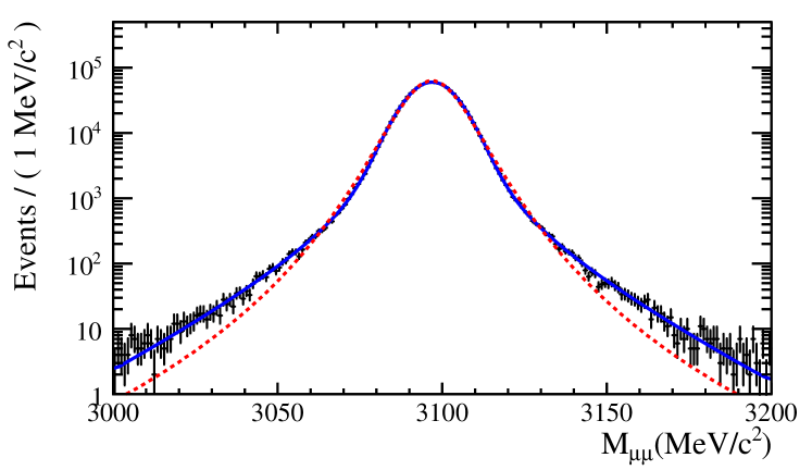
can provide a better fit than I(m,μ,σ,λ,ζ,β,a,n)𝐼𝑚𝜇𝜎𝜆𝜁𝛽𝑎𝑛I(m,\mu,\sigma,\lambda,\zeta,\beta,a,n) for some complicated cases with high statistics, without a real increase in the number of fit parameters (v0subscript𝑣0\sqrt{v_{0}} can be fixed in a somewhat arbitrary point at the start-up of the mass error distribution), although at the cost of a numerical convolution. The later can be done in RooFit by calling the RooFFTConvPdf class on top of the implementation of I(m,μ,σ,λ,ζ,β,a,n)𝐼𝑚𝜇𝜎𝜆𝜁𝛽𝑎𝑛I(m,\mu,\sigma,\lambda,\zeta,\beta,a,n). If written this way, v0subscript𝑣0\sqrt{v_{0}} can be interpreted as an estimate of the mass resolution due to multiple scattering, σSRsuperscript𝜎𝑆𝑅\sigma^{SR} the dispersion caused by the spatial resolution of the detector given the kinematics of the final state, and the total resolution would be σ=v0+(σSR)2𝜎subscript𝑣0superscriptsuperscript𝜎𝑆𝑅2\sigma=\sqrt{v_{0}+(\sigma^{SR})^{2}}. Fig. 6 shows a fit of I(m,μ,σ,λ,ζ,0,,1)𝐼𝑚𝜇𝜎𝜆𝜁01I(m,\mu,\sigma,\lambda,\zeta,0,\infty,1) and Υ(m,μ,σSR,λ,ζ,0,,1,6.5MeV/c2)Υ𝑚𝜇superscript𝜎𝑆𝑅𝜆𝜁016.5MeVsuperscript𝑐2\Upsilon(m,\mu,\sigma^{SR},\lambda,\zeta,0,\infty,1,6.5\,{\rm MeV}/c^{2}) to the simulated J/ψμ+μ𝐽𝜓superscript𝜇superscript𝜇J/\psi\to\mu^{+}\mu^{-} data, for the full sample without any kinematic constraint, i.e., where very low momentum (MS dominated) and very high momentum (hit resolution dominated) coexist. The fitting range corresponds to about eleven standard deviations. An excellent agreement between Υ(m,μ,σSR,λ,ζ,0,,1,6.5MeV/c2)Υ𝑚𝜇superscript𝜎𝑆𝑅𝜆𝜁016.5MeVsuperscript𝑐2\Upsilon(m,\mu,\sigma^{SR},\lambda,\zeta,0,\infty,1,6.5\,{\rm MeV}/c^{2}) and the simulated data is found. We failed to find any subsample of the J/ψμ+μ𝐽𝜓superscript𝜇superscript𝜇J/\psi\to\mu^{+}\mu^{-} data that could not be fitted by Υ(m,μ,σSR,λ,ζ,0,,1,v0)Υ𝑚𝜇superscript𝜎𝑆𝑅𝜆𝜁01subscript𝑣0\Upsilon(m,\mu,\sigma^{SR},\lambda,\zeta,0,\infty,1,v_{0}).

Refer to caption
Figure 6: Fit of I(m,μ,σ,λ,ζ,0,,1)𝐼𝑚𝜇𝜎𝜆𝜁01I(m,\mu,\sigma,\lambda,\zeta,0,\infty,1) (red dashed) and Υ(m,μ,σSR,λ,ζ,0,,1,6.5MeV/c2)Υ𝑚𝜇superscript𝜎𝑆𝑅𝜆𝜁016.5MeVsuperscript𝑐2\Upsilon(m,\mu,\sigma^{SR},\lambda,\zeta,0,\infty,1,6.5\,{\rm MeV}/c^{2}) (solid blue) to the simulated J/ψμ+μ𝐽𝜓superscript𝜇superscript𝜇J/\psi\to\mu^{+}\mu^{-} data, for the full sample without any kinematic constraint.

6 Properties of λ𝜆\lambda

We have seen that using the Hypatia ΥΥ\Upsilon distribution we can factorize the mass resolution modelling into MS and SR. The first part is governed by a resolution parameter σ0subscript𝜎0\sigma_{0} that can be estimated from the start-up of the per-event variance distribution. The second part is governed by the parameters ζ,λ,σ𝜁𝜆𝜎\zeta,\lambda,\sigma of the generalized hyperbolic distribution, where σ𝜎\sigma corresponds to the resolution introduced by SR and where, empirically, we have found that ζ𝜁\zeta is in most cases small. In this chapter we will derive a physical meaning for λ𝜆\lambda, at least in the small ζ𝜁\zeta limit.

In the α=0𝛼0\alpha=0 (ζ=0absent𝜁0\rightarrow\zeta=0) limit case, the generalized hyperbolic distribution becomes a Student’s-t distribution, which can be understood as a marginalization over a per-event variance density:

ρ(v)vλ1eb/vproportional-to𝜌𝑣superscript𝑣𝜆1superscript𝑒𝑏𝑣\rho(v)\propto v^{\lambda-1}e^{-b/v} (16)

The mean (M𝑀M) and mode (μ𝜇\mu) of (16) are:

M=bλ1;μ=bλ+1formulae-sequence𝑀𝑏𝜆1𝜇𝑏𝜆1M=\frac{b}{-\lambda-1};\mu=\frac{b}{-\lambda+1} (17)

thus

λ=1+M(v)/μ(v)1M(v)/μ(v)<0𝜆1𝑀𝑣𝜇𝑣1𝑀𝑣𝜇𝑣0\lambda=\frac{1+M(v)/\mu(v)}{1-M(v)/\mu(v)}<0 (18)

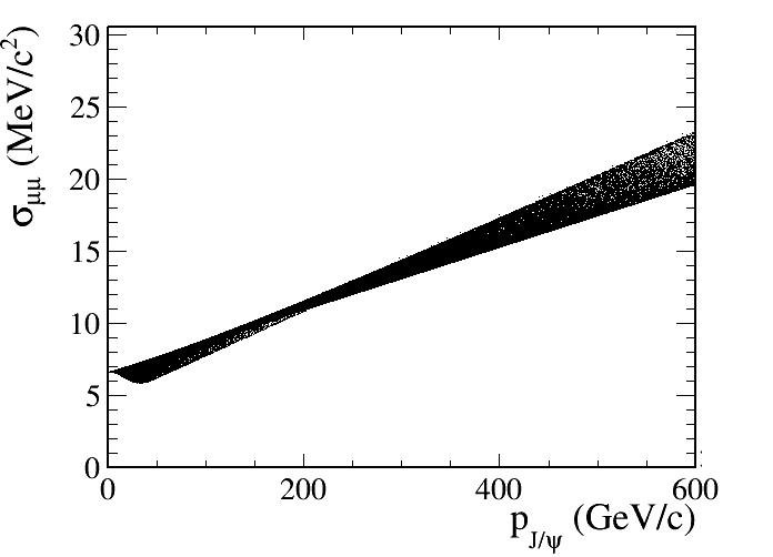
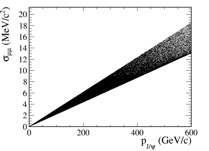
and we can get an estimate of λ𝜆\lambda by looking at the per-event error (squared) distribution, and making the ratio of its mean and mode after shifting it to start at zero. But, we can further exploit this relation. From (3) we can suppose that the per-event uncertainty will be strongly correlated with the particle momenta. Indeed, Fig. 7 supports this.

σiSRcte×pJ/ψ,isuperscriptsubscript𝜎𝑖𝑆𝑅subscript𝑐𝑡𝑒subscript𝑝𝐽𝜓𝑖\sigma_{i}^{SR}\approx c_{te}\times p_{J/\psi,i} (19)

If this is the case, then M(vSR)/μ(vSR)M(pJ/ψ2)/μ(pJ/ψ2)𝑀superscript𝑣𝑆𝑅𝜇superscript𝑣𝑆𝑅𝑀superscriptsubscript𝑝𝐽𝜓2𝜇superscriptsubscript𝑝𝐽𝜓2M(v^{SR})/\mu(v^{SR})\approx M(p_{J/\psi}^{2})/\mu(p_{J/\psi}^{2}) and λ𝜆\lambda does not depend on detector effects, only on particle kinematics. This is an interesting result, because if we have a MC simulation with a good description of the momentum distribution of the particles in the lab frame, then the values of λ𝜆\lambda obtained in simulation should be reasonably valid for data, regardless of having an accurate description of detector simulation.
Refer to caption
Refer to caption
Figure 7: Per-event mass uncertainty versus J/ψ𝐽𝜓J/\psi momentum. Left: with multiple scattering. Right: only detector resolution.
Table 2: Results of a fit to Υ(m,μ,σSR,λ,0,0,,1,σMS)Υ𝑚𝜇superscript𝜎𝑆𝑅𝜆001superscript𝜎𝑀𝑆\Upsilon(m,\mu,\sigma^{SR},\lambda,0,0,\infty,1,\sigma^{MS}) for toy MC J/ψ𝐽𝜓J/\psi events smeared with different values of a𝑎a and b𝑏b in (3). The parameter σMSsuperscript𝜎𝑀𝑆\sigma^{MS} is fixed at the start-up of the per-event variance. The parameter λ𝜆\lambda is found to be very stable with respect to smearing parameters, which are varied by 100%percent100100\%. However the uncertainty on λ𝜆\lambda varies significantly, and increases with a/b𝑎𝑏a/b.
a[×103][\times 10^{-3}] b GeV/c1GeVsuperscript𝑐1\,{\rm GeV}/c^{-1} λ𝜆\lambda σMS(MeV/c2)superscript𝜎𝑀𝑆MeVsuperscript𝑐2\sigma^{MS}(\,{\rm MeV}/c^{2}) σSR(MeV/c2)superscript𝜎𝑆𝑅MeVsuperscript𝑐2\sigma^{SR}(\,{\rm MeV}/c^{2})
3 2×10⁵absentsuperscript105\times 10^{-5} 2.40±0.06plus-or-minus2.400.06-2.40\pm 0.06 6.81 4.75±0.02plus-or-minus4.750.024.75\pm 0.02
1.5 2×10⁵absentsuperscript105\times 10^{-5} 2.10±0.03plus-or-minus2.100.03-2.10\pm 0.03 3.53 3.71±0.01plus-or-minus3.710.013.71\pm 0.01
6 2×10⁵absentsuperscript105\times 10^{-5} 2.67±0.16plus-or-minus2.670.16-2.67\pm 0.16 13.3 6.3±0.05plus-or-minus6.30.056.3\pm 0.05
3 4×10⁵absentsuperscript105\times 10^{-5} 2.11±0.03plus-or-minus2.110.03-2.11\pm 0.03 7.07 7.53±0.03plus-or-minus7.530.037.53\pm 0.03
3 1×10⁵absentsuperscript105\times 10^{-5} 2.65±0.15plus-or-minus2.650.15-2.65\pm 0.15 6.67 3.06±0.03plus-or-minus3.060.033.06\pm 0.03

7 Mass constraints on intermediate resonances

Up to now we have described resolution effects. In more complicated cases, it is sometimes very useful to apply constraints on the decay products. For example, one can significantly improve the invariant mass resolution of Bs0J/ψϕsubscriptsuperscript𝐵0𝑠𝐽𝜓italic-ϕB^{0}_{s}\to J/\psi\phi by constraining the two muons to have the PDG J/ψ𝐽𝜓J/\psi mass [9]. This kind of approach, although great at improving the overall resolution, can also generate tails on the mass distribution, due to the photon energy radiated in the J/ψμ+μ𝐽𝜓superscript𝜇superscript𝜇J/\psi\to\mu^{+}\mu^{-} decay. Let’s consider a simple case in which the constraint is just applied by substituting the mass of the dimuon by the mass of the J/ψ𝐽𝜓J/\psi.

mc2=mJ/ψ2+mKK2+2(mJ/ψ2+pμμ2mKK2+pKK2pμμpKKcos(θ))superscriptsubscript𝑚𝑐2superscriptsubscript𝑚𝐽𝜓2superscriptsubscript𝑚𝐾𝐾22superscriptsubscript𝑚𝐽𝜓2superscriptsubscript𝑝𝜇𝜇2superscriptsubscript𝑚𝐾𝐾2superscriptsubscript𝑝𝐾𝐾2subscript𝑝𝜇𝜇subscript𝑝𝐾𝐾𝜃m_{c}^{2}=m_{J/\psi}^{2}+m_{KK}^{2}+2\left(\sqrt{m_{J/\psi}^{2}+p_{\mu\mu}^{2}}\sqrt{m_{KK}^{2}+p_{KK}^{2}}-p_{\mu\mu}p_{KK}\cos(\theta)\right) (20)

while ideally one would have wanted to implement:

mtrue2=mJ/ψ2+mKK2+2(mJ/ψ2+pJ/ψ2mKK2+pKK2pJ/ψpKKcos(θ))superscriptsubscript𝑚𝑡𝑟𝑢𝑒2superscriptsubscript𝑚𝐽𝜓2superscriptsubscript𝑚𝐾𝐾22superscriptsubscript𝑚𝐽𝜓2superscriptsubscript𝑝𝐽𝜓2superscriptsubscript𝑚𝐾𝐾2superscriptsubscript𝑝𝐾𝐾2subscript𝑝𝐽𝜓subscript𝑝𝐾𝐾𝜃m_{true}^{2}=m_{J/\psi}^{2}+m_{KK}^{2}+2\left(\sqrt{m_{J/\psi}^{2}+p_{J/\psi}^{2}}\sqrt{m_{KK}^{2}+p_{KK}^{2}}-p_{J/\psi}p_{KK}\cos(\theta)\right) (21)

The difference mc2mtrue2superscriptsubscript𝑚𝑐2superscriptsubscript𝑚𝑡𝑟𝑢𝑒2m_{c}^{2}-m_{true}^{2} is not zero but rather function of the energy of the photons generated in the J/ψμ+μ𝐽𝜓superscript𝜇superscript𝜇J/\psi\to\mu^{+}\mu^{-} decay. This difference can be greater than zero, generating a tail on the right-hand side. Hence, even with a perfect detector resolution, the combination of the mass constraint and the photon radiation will generate non-Gaussian tails. In practice, this effect is expected to be small because the J/ψμ+μ𝐽𝜓superscript𝜇superscript𝜇J/\psi\to\mu^{+}\mu^{-} decays are selected with a mass window cut that allows only low energy photons. Otherwise, it can be partially accommodated either by the resolution model (e.g (8)) or by using a CB-like tail on the right-hand side (i.e, using a double-sided Hypatia). A further discussion that goes beyond the scope of this paper is to provide models marginalized over per-event errors.

8 Conclusions

We have presented a generalization of the Crystal Ball function that gives an excellent description of mass resolution non-Gaussian tails. This function, that we name the Hypatia distribution, I𝐼I, corresponds to a CB-like tail with a generalized hyperbolic core. The smeared Hypatia distribution, ΥΥ\Upsilon provides an improved description of mass peaks and its fit parameters have clearer fundamental meaning, although the price to pay is a numeric convolution. A second, right-hand side CB-like tail can be added in cases where one has other non-resolution effects, such as those coming from constraining the mass of intermediate resonances of a decay.

9 Acknowledgments

We would like to thank L. Carson and V. Gligorov for his useful comments on this draft. We would also like to thank W. Hulsbergen for helpful discussions during the preparation of this work.

References

  • [1] M. Oreglia, A Study of the Reactions ψγγψsuperscript𝜓𝛾𝛾𝜓\psi^{\prime}\to\gamma\gamma\psi, Ph.D. thesis (1980).
  • [2] J. Gaiser, Charmonium Spectroscopy From Radiative Decays of the J/ψ𝐽𝜓J/\psi and ψsuperscript𝜓\psi^{\prime}, Ph.D. thesis (1982).
  • [3] T. Skwarnicki, A study of the radiative cascade transitions between the Upsilon-prime and Upsilon resonances, Ph.D. thesis, Institute of Nuclear Physics, Krakow, DESY-F31-86-02 (1986).
  • [4] T. Sjöstrand, S. Mrenna, P. Skands, PYTHIA 6.4 physics and manual, JHEP 05 (2006) 026. arXiv:hep-ph/0603175, doi:10.1088/1126-6708/2006/05/026.
  • [5] A. A. Alves Jr., et al., The LHCb detector at the LHC, JINST 3 (2008) S08005. doi:10.1088/1748-0221/3/08/S08005.
  • [6] R. Aaij, et al., Measurement of CP𝐶𝑃CP violation and the Bs0superscriptsubscript𝐵𝑠0B_{s}^{0} meson decay width difference with Bs0J/ψK+Ksuperscriptsubscript𝐵𝑠0𝐽𝜓superscript𝐾superscript𝐾B_{s}^{0}\to J/\psi K^{+}K^{-} and Bs0J/ψπ+πsuperscriptsubscript𝐵𝑠0𝐽𝜓superscript𝜋superscript𝜋B_{s}^{0}\to J/\psi\pi^{+}\pi^{-} decays, Phys.Rev. D87 (2013) 112010. arXiv:1304.2600, doi:10.1103/PhysRevD.87.112010.
  • [7] L. Amoroso, Richerche intorno alla curve die redditi, Ann. Mat. Pura. Appl. 21 (1925) 123–159.
  • [8] A. J. McNeil, R. Frey, P. Embrechts, Quantitative Risk Management Concepts, Techniques and Tools, Princeton University Press.
  • [9] J. Beringer, et al., Review of particle physics, Phys. Rev. D86 (2012) 010001. doi:10.1103/PhysRevD.86.010001.