Constraints on Gauge Field Production
during Inflation

In order to gain new insights into the gauge field couplings in the early universe, we consider the constraints on gauge field production during inflation imposed by requiring that their effect on the CMB anisotropies are subdominant. In particular, we calculate systematically the bispectrum of the primordial curvature perturbation induced by the presence of vector gauge fields during inflation. Using a model independent parametrization in terms of magnetic non-linearity parameters, we calculate for the first time the contribution to the bispectrum from the cross correlation between the inflaton and the magnetic field defined by the gauge field. We then demonstrate that in a very general class of models, the bispectrum induced by the cross correlation between the inflaton and the magnetic field can be dominating compared with the non-Gaussianity induced by magnetic fields when the cross correlation between the magnetic field and the inflaton is ignored.

1 Introduction

Recent data from the Planck satellite has verified the paradigm of single field slow roll inflation to unprecedented high precision [1, 2]. This alone is a great success, but it also provides new nontrivial constraints on other degrees of freedom, which we either know are there in the post-inflationary universe (neutrinos [3, 4, 5, 6, 7], magnetic fields [8, 9, 10, 11], dark matter [12, 13, 14, 15, 16], dark energy [17, 18, 19, 20], etc.) or which we have some reasons to believe could be present even during inflation, such as in multi-field models of inflation [21, 22], the curvaton model [23, 24, 25], or models of inflationary magnetogenesis [26, 27, 28, 29, 30, 31, 32, 33]. In the present paper we will focus on the constraints imposed on a $U(1)$ vector field coupled to the inflaton, coming from the observational constraints on non-Gaussianity in the CMB. For the applications in this paper, this could be a completely general $U(1)$ vector field, but the applications of the results presented below are especially interesting when one identifies the vector field with the one of elect! romagnetism.

Cosmic magnetic fields with a coherent scale as large as 100 kpc and a strength of order $\mu$G has been established to be present in galaxies and clusters of galaxies [34, 35, 36]. It is believed that the origin of such magnetic fields might be due to an enhancement of pre-existing small magnetic fields, called seed fields, due to the dynamo mechanism. It is generally assumed that these seed fields need to have a strength larger than about $10^{-20}$ Gauss in order for the dynamo mechanism to work [26], although it has been claimed that this lower bound can be significantly relaxed in the presence of dark energy [37]. Two possible explanations for the origin of such seeds exists. One is the possibility that conformal invariance of electro-magnetism is broken sufficiently during inflation, in order to enhance quantum fluctuations of the $U(1)$ vector field and generate the seed magnetic fields at the end o! f inflation [26, 27, 28, 29, 30, 31, 32]. Another possibility is that the seeds are generated after inflation, f.ex. during a phase transition or from the Bierman battery mechanism [10]. Recently there has however been a claimed indirect observation of femto Gauss magnetic fields with a coherence length of super Mpc scales [38, 39, 40]. If this is true, this could pose a problem for mechanisms which generates the magnetic seeds by causal processes after inflation, since the coherence length of such magnetic fields are limited by the horizon at the time of generation, and is typically too small to explain magnetic fields with a coherence length larger than the Mpc scale. This might suggest that the magnetic seeds are generated during inflation.

However, it is a challenge for inflationary magnetogenesis to identify a source that breaks sufficiently the conformal invariance of electro-magnetism during inflation. If the conformal invariance would be unbroken, then the vector field perturbation would not get enhanced during inflation, and no significant magnetic fields would be generated. One of the simplest and most popular models for breaking the conformal invariance during inflation is to add a non-minimal coupling between the gauge kinetic term $F_{\mu\nu}F^{\mu\nu}$ and the inflaton, $\phi$, of the form $\lambda(\phi)F_{\mu\nu}F^{\mu\nu}$ [26, 27, 28, 29, 30, 31, 32]. Backreaction provides a simple constraint on the magnetic field generated during inflation in this type of models, although in principle inflationary attractor solutions dominated by the gauge field energy density may also exist [41]. In order not to disturb the standard inflationary picture we must require that the energy density in the magnetic field $\rho_{B}$ is smaller than the total energy density $\rho$ during inflation, while at the same time staying in a perturbative regime in order to avoid the strong coupling problem [42, 43]. In fact, it has been demonstrated that the generation of significant seed magnetic fields from inflation seems to require low-scale inflation [43]. However, the fluctuating magnetic field also contributes to the total curvature perturbation, $\zeta$, and since the perturbations from the magnetic field are non-Gaussian this leads to additional strong constraints on the strength of magnetic fields generated during inflation [44, 45, 46].

In addition, due to the non-minimal coupling between the inflaton and the vector field, models of the type $\lambda(\phi)F_{\mu\nu}F^{\mu\nu}$ will also induce non-trivial correlations between the inflation fluctuations and the magnetic field. Such cross correlations was recently studied in [47, 48, 49, 50, 51, 52], and in [49] it was suggested that such cross correlations could be parametrized in a model independent way in terms of a magnetic non-linearity parameter, $b_{NL}$ of the form $\left<\zeta~{}{\bf B}\cdot{\bf B}\right>\propto b_{NL}P_{\zeta}P_{B}$ analogous to the definition of $f_{NL}$, where here $P_{\zeta}$ and $P_{B}$ are the power spectra of the curvature perturbation and the magnetic field respectively. In fact one can derive a new “magnetic consistency relation” in terms of the parameter $b_{NL}$ [49, 50]

In the work presented here, we will analyze the induced non-Gaussianity in the CMB from such cross-correlations between the inflation fluctuations and the magnetic field in the general class of models where the gauge field action takes the form

$${\cal L}_{\rm gauge}=\lambda(\phi)F_{\mu\nu}F^{\mu\nu}\ .$$ (1.1)

The general analysis allows to use the level of induced non-Gaussianity to constrain the possible forms of the coupling $\lambda(\phi)$. As a benchmark model, we will also calculate the induced non-Gaussianity from cross-correlations in the extensively studied models where the coupling $\lambda(\phi)$ takes a power law form. This new contribution which will turn out to be the dominant non-Gaussian contribution in certain shapes.

As already mentioned above, the non-Gaussianity induced by the magnetic field, when ignoring the cross-correlations with the inflaton, has already been studied extensively the literature in the specific $\lambda(\phi)F_{\mu\nu}F^{\mu\nu}$ models with a power law coupling $\lambda(\phi)$ [44, 45, 46]. In order to understand the relation between the different results in the literature and the results presented here, let us write the total curvature perturbation in terms of the curvature perturbation in the inflaton fluid, $\zeta_{\phi}$, and in the magnetic field fluid, $\tilde{\zeta}_{B}$, as

$$\zeta=-H\frac{\delta\rho_{\phi}+\delta\rho_{B}}{\dot{\rho}}\equiv\zeta_{\phi}+\tilde{\zeta}_{B}\ .$$ (1.2)

At the background level $\rho=\rho_{\phi}$ as we assume a vanishing v.e.v. for the magnetic field. However, at first order in perturbations the average energy density of the magnetic field fluctuations gives an effective background component $\rho_{B}\equiv\langle\delta\rho_{B}\rangle$. Considering fluctuations over the average value we can define the intrinsic curvature perturbation of the magnetic fluid as

$$\hat{\zeta}_{B}=\frac{\dot{\rho}_{\phi}}{\dot{\rho}_{B}}\tilde{\zeta}_{B}\ .$$ (1.3)

Consider the time derivative of $\zeta$, to see how it grows with time. It is well known that in the absence of direct coupling between the fluids, the curvature perturbation in each fluid is separately conserved on superhorizon scales and we have $\dot{\zeta}_{\phi}\simeq\dot{\hat{\zeta}}_{B}\simeq 0$, while in the presence of sources we have

$$\dot{\delta\rho_{\phi}}+3H(\delta\rho_{\phi}+\delta p_{\phi}) = -Q$$

$$\dot{\delta\rho_{B}}+3H(\delta\rho_{B}+\delta p_{B}) = Q\ .$$ (1.4)

From the continuity equation of the electromagnetic field in the regime where the magnetic fields dominates the electromagnetic energy density, we have [50]

$$\dot{\delta\rho_{B}}+4H\delta\rho_{B}=\frac{\dot{\lambda}}{\lambda}\delta\rho_{B}\ ,$$ (1.5)

it follows that the energy transfer term is given by

$$Q=\frac{\dot{\lambda}}{\lambda}\delta\rho_{B}\ .$$ (1.6)

From (1) it follows that

$$\dot{\zeta}_{\phi} = 3\frac{H^{2}}{\dot{\rho}_{\phi}}(\delta p_{\phi}-\frac{\dot{p}_{\phi}}{\dot{\rho}_{\phi}}\delta\rho_{\phi})+H\frac{Q}{\dot{\rho}_{\phi}}\approx H\frac{Q}{\dot{\rho}_{\phi}}$$

$$\dot{\hat{\zeta}}_{B} = 3\frac{H^{2}}{\dot{\rho}_{B}}(\delta p_{B}-\frac{\dot{p}_{B}}{\dot{\rho}_{B}}\delta\rho_{B})-H\frac{Q}{\dot{\rho}_{B}}-\frac{\dot{Q}}{\dot{\rho}_{B}}\hat{\zeta}_{B}\approx-H\frac{Q}{\dot{\rho}_{B}}-\frac{\dot{Q}}{\dot{\rho}_{B}}\hat{\zeta}_{B}\$$ (1.7)

where in the last steps we assumed that the intrinsic non-adiabatic pressure in the two fluids vanishes. We have also neglected slow roll suppressed terms proportional to ${\dot{H}}$.

Now we can compute $\dot{\tilde{\zeta}}_{B}$, which gives

$$\dot{\tilde{\zeta}}_{B} = -H\frac{Q}{\dot{\rho}_{\phi}}-\frac{H}{\rho_{\phi}+p_{\phi}}\left(\delta p_{B}-\frac{\dot{p}_{\phi}}{\dot{\rho}_{\phi}}\delta\rho_{B}\right)$$ (1.8)

$$\equiv -H\frac{Q}{\dot{\rho}_{\phi}}-\frac{H}{{\rho}_{\phi}+{p}_{\phi}}\delta P_{nad}~{}.$$

Thus, clearly if we were to compute $\dot{\zeta}$, the source term, $Q$, cancels out and we obtain

$$\dot{\zeta}=\dot{\zeta}_{\phi}+\dot{\tilde{\zeta}}_{B}=-\frac{H}{\rho+p}\delta P_{nad}.$$ (1.9)

This is in agreement with [46], but in general inconsistent with assuming $\dot{\tilde{\zeta}}_{B}=0$ and considering only the source term on $\zeta_{\phi}$ as in [44, 45] (see appendix A for further discussion of this point). From equation (1) we see that the curvature perturbations of the inflaton fluid and the magnetic fluid evolve only if the coupling $\lambda$ is changing in time. However, as the total curvature perturbation (1.2) is not just a sum of $\zeta_{\phi}$ and $\hat{\zeta}_{B}$ but their sum weighted by the ratios of the individual fluid energies the curvature perturbation evolves even if $\zeta_{\phi}$ and $\hat{\zeta}_{B}$ are constant but the fluid energies $\rho_{\phi}$ and $\rho_{B}$ evolve differently.

As we will discuss in section 4, the non-adiabatic pressure, $\delta P_{nad}$, is proportional to the strength of the magnetic field squared, $B^{2}$. By integration of equation (1.9), we see that there are two distinct contributions to the curvature perturbation. There is a contribution proportional to the magnetic field squared, $B^{2}$, obtained by integrating the the non-adiabtic pressure on super-horizon scales, which we will label $\zeta_{B}$. In addition there is a constant of integration which is the contribution to the curvature perturbation at horizon crossing, which is independent of the magnetic field and given by the inflation fluctuation. We will label this constant of integration $\zeta_{0}$. We can the write the total curvature perturbation simply as

$$\zeta=\zeta_{0}+\zeta_{B}~{},$$ (1.10)

where $\zeta_{0}$ is given by $\zeta_{\phi}$ evaluated at horizon crossing, and $\zeta_{B}$ is the super-horizon contribution determined by the non-adiabatic pressure, which is proportional to $B^{2}$.

While the correlation function

$$\left<\zeta_{B}\zeta_{B}\zeta_{B}\right>$$ (1.11)

which contributes to the observable $\langle\zeta\zeta\zeta\rangle$, parameterized by the non-linearity parameter $f_{NL}$, was computed in [46] (see also [44, 45]), the correlation between $\zeta_{0}$ and $\zeta_{B}$ is to our knowledge neglected in all of the previous work. As can be seen from equation (1.10), the three point function of the total curvature perturbation $\zeta$ also receives contributions from terms of the form

$$\left<\zeta_{0}\zeta_{B}\zeta_{B}\right>~{},\qquad\left<\zeta_{0}\zeta_{0}\zeta_{B}\right>~{}.$$ (1.12)

The main point of this paper is to calculate the cross correlation contributions. In section 4, we will see that these terms can give the dominant contribution to the observable $\langle\zeta\zeta\zeta\rangle$, even larger than the contribution

from $\left<\zeta_{B}\zeta_{B}\zeta_{B}\right>$ computed in [46]. Since $\delta P_{nad}$ is proportional to the strength of the magnetic field squared, $B^{2}$, the correlators of the type shown in (1.12) will be given in terms of cross correlation function of the magnetic field with the curvature perturbation

$$\left<\zeta_{0}\zeta_{0}B^{2}\right>~{},\qquad\left<\zeta_{0}B^{2}B^{2}\right>~{}.$$ (1.13)

In a specific model these correlators will have to be computed in the in-in formalism [53] going beyond linear perturbation theory, which for every new model can a tedious calculation. However, in the next section, we will discuss how these correlation functions can be parametrized in terms of magnetic non-linearity parameters in a model independent way, and in section 3 we will show how to evaluate them.

The paper is organized as follows. In the next section introduce the magnetic non-linearity parameters, and show how the cross correlation functions of the curvature perturbation with the magnetic field can be parametrized in a model independent way. In section 3 we evaluate these model independent cross-correlation functions. In section 4, we find the induced non-Gaussinity from the cross correlation functions, and in section 5 we also consider the size of these cross correlation functions in the specific models where the coupling $\lambda(\phi)$ in $\lambda(\phi)F_{\mu\nu}F^{\mu\nu}$ takes a power law form. Finally, in section 6, we conclude and summarize our results.

2 The magnetic non-linearity parameters

If we define the cross-correlation bispectrum of the curvature perturbation with the magnetic fields as

$$\left<\zeta_{0}(\bm{\mathrm{{k}}}_{1}){\bf B}(\bm{\mathrm{{k}}}_{2})\cdot{\bf B}(\bm{\mathrm{{k}}}_{3})\right>\equiv(2\pi)^{3}\delta^{(3)}(\bm{\mathrm{{k}}}_{1}+\bm{\mathrm{{k}}}_{2}+\bm{\mathrm{{k}}}_{3})B_{\zeta BB}(\bm{\mathrm{{k}}}_{1},\bm{\mathrm{{k}}}_{2},\bm{\mathrm{{k}}}_{3})~{},$$ (2.1)

then is has previously been proposed, that it is convenient to define the magnetic non-linearity parameter $b_{NL}$, in terms of the cross-correlation function of the curvature perturbation with the magnetic fields

$$B_{\zeta BB}(\bm{\mathrm{{k}}}_{1},\bm{\mathrm{{k}}}_{2},\bm{\mathrm{{k}}}_{3})\equiv\frac{1}{2}b_{NL}P_{\zeta}(k_{1})\left(P_{B}(k_{2})+P_{B}(k_{3})\right)~{},$$ (2.2)

where $P_{\zeta}$ and $P_{B}$ are the power spectra of the comoving curvature perturbation and the magnetic fields, defined respectively as

$$\left<\zeta(\bm{\mathrm{{k}}})\zeta(\bm{\mathrm{{k}}}^{\prime})\right>\equiv(2\pi)^{3}\delta^{(3)}(\bm{\mathrm{{k}}}+\bm{\mathrm{{k}}}^{\prime})P_{\zeta}(k),$$ (2.3)

$$\left<{\bf B}(\bm{\mathrm{{k}}})\cdot{\bf B}(\bm{\mathrm{{k}}}^{\prime})\right>\equiv(2\pi)^{3}\delta^{(3)}(\bm{\mathrm{{k}}}+\bm{\mathrm{{k}}}^{\prime})P_{B}(k).$$ (2.4)

Similarly we may also introduce the magnetic trispectrum

$$\left<\zeta_{0}(\bm{\mathrm{{k}}}_{1})\zeta_{0}(\bm{\mathrm{{k}}}_{2}){\bf B}(\bm{\mathrm{{k}}}_{3})\cdot{\bf B}(\bm{\mathrm{{k}}}_{4})\right>\equiv(2\pi)^{3}\delta^{(3)}(\bm{\mathrm{{k}}}_{1}+\bm{\mathrm{{k}}}_{2}+\bm{\mathrm{{k}}}_{3}+\bm{\mathrm{{k}}}_{4})T_{\zeta\zeta BB}(\bm{\mathrm{{k}}}_{1},\bm{\mathrm{{k}}}_{2},\bm{\mathrm{{k}}}_{3},\bm{\mathrm{{k}}}_{4})~{},$$ (2.5)

which can be parametrized in terms of new magnetic non-linearity parameters $\beta_{NL}$ and $c_{NL}$,

$$T_{\zeta\zeta BB}(\bm{\mathrm{{k}}}_{1},\bm{\mathrm{{k}}}_{2},\bm{\mathrm{{k}}}_{3},\bm{\mathrm{{k}}}_{4})\equiv\beta_{NL}P_{\zeta}(k_{1})P_{\zeta}(k_{2})P_{B}(k_{13})+\frac{2}{3}c_{NL}P_{\zeta}(k_{1})P_{\zeta}(k_{2})P_{B}(k_{4})~{}+perm.,$$ (2.6)

In the case where $b_{NL}$ is momentum independent and quantum interference effects around horizon crossing can be ignored, it takes a “local” form which can be derived from the relation

$${\bf B}={\bf B}^{(G)}+\frac{1}{2}b_{NL}^{local}\zeta_{0}{\bf B}^{(G)}+\frac{1}{6}c_{NL}^{local}\zeta_{0}\zeta_{0}{\bf B}^{(G)}$$ (2.7)

with ${\bf B}^{(G)}$ and $\zeta_{0}$ being Gaussian fields. With this local ansatz one obtains that the $\beta_{NL}$ term in the trispectrum is given by

$$\beta^{local}_{NL}=\frac{1}{2}(b^{local}_{NL})^{2}~{}.$$ (2.8)

There are interesting limits where indeed the magnetic bispetrum and trispectrum can be derived from semiclassical considerations, and in these ”squeezed” limits the magnetic non-linearity parameter takes the local form. It has previously been shown that in the squeezed limit, where the momentum of the curvature perturbation vanishes, i.e., $k_{1}\ll k_{2},k_{3}$, the bispectrum in fact takes the form

$$\left<\zeta_{0}(\bm{\mathrm{{k}}}_{1}){\bf B}(\bm{\mathrm{{k}}}_{2})\cdot{\bf B}(\bm{\mathrm{{k}}}_{3})\right>=b_{NL}^{local}(2\pi)^{3}\delta^{(3)}(\bm{\mathrm{{k}}}_{1}+\bm{\mathrm{{k}}}_{2}+\bm{\mathrm{{k}}}_{3})P_{\zeta}(k_{1})P_{B}(k_{2})~{},$$ (2.9)

with $b_{NL}^{local}=n_{B}-4$ where $n_{B}$ is the spectral index of the magnetic field power spectrum, in agreement with the magnetic consistency relation, which was derived in [49, 50]. In the case of a scale invariant spectrum of magnetic fields, $n_{B}=0$, we have $b^{local}_{NL}=-4$ (see also appendix B).

Another interesting limit which maximizes the three-point cross-correlation function is the flattened shape where $k_{1}/2=k_{2}=k_{3}$. In this limit it turns out that the signal is enhanced by a logarithmic factor in agreement with [47, 48, 49, 50]. On the largest scales the logarithm will give an enhancement by a factor 60. Thus, for a flat magnetic field power spectrum, the non-linearity parameter in the flattened limit becomes $|b_{NL}|\sim\mathcal{O}(10^{3})$ depending on the scale.

3 Three-point cross-correlation functions

Since the electromagnetic part of the perturbed action contains only terms of the form $A^{2}\zeta^{n}$, see equation (1.1), the curvature perturbation generated the magnetic fields is of the form $\zeta_{B}\propto B_{i}B^{i}/(H^{2}M_{\rm P}^{2})$. The magnetic fields generated during inflation obey a Gaussian statistics to leading order in perturbations so that the induced curvature perturbation $\zeta_{{\rm B}}$ is a non-Gaussian field.

To estimate the contribution of magnetic fields to the bispectrum of primordial density fluctuations we should consider three-point functions of the form.

$$\langle\zeta_{0}(\bm{\mathrm{{k}}}_{1})\zeta_{0}(\bm{\mathrm{{k}}}_{2}){\bf B}^{2}(\bm{\mathrm{{k}}}_{3})\rangle\ ,\qquad\langle\zeta_{0}(\bm{\mathrm{{k}}}_{1}){\bf B}^{2}(\bm{\mathrm{{k}}}_{2}){\bf B}^{2}(\bm{\mathrm{{k}}}_{3})\rangle\ ,\qquad\langle{\bf B}^{2}(\bm{\mathrm{{k}}}_{1}){\bf B}^{2}(\bm{\mathrm{{k}}}_{2}){\bf B}^{2}(\bm{\mathrm{{k}}}_{3})\rangle\ .$$ (3.1)

To lowest order in perturbations, the amplitudes of the two first correlators depend on the parameters $b_{\rm NL}$ and $c_{\rm NL}$ in the expansion (2.7) while the last correlator only depends on the amplitude of magnetic fields.

The two-point function of the magnetic fields is given to lowest order in perturbations by,

$$\langle B_{i}({\bf k})B_{j}({\bf k}^{\prime})\rangle=(2\pi)^{3}\delta({\bf k}+{\bf k}^{\prime})\frac{1}{2}\left(\delta_{ij}-\frac{k_{i}k_{j}}{k^{2}}\right)P_{{\rm B}}(k)\ .$$ (3.2)

For simplicity, we assume the scale and time dependence of the magnetic spectrum can be parameterized by a power law as

$$P_{B}(k)=\frac{C_{B}}{\lambda(\eta)}(-k\eta)^{4-2n}k^{-3}\ ,$$ (3.3)

where $C_{B}$ is a constant. The power law spectrum of magnetic fields is obtained in the extensively studied class of models with ${\cal L}=\lambda(\phi)F_{\mu\nu}F^{\mu\nu}$ and a power law form for the coupling $\lambda\propto a^{n}$. However, in this case the coefficients $b_{\rm NL}$ and $c_{\rm NL}$, which are determined by the derivatives of the coupling $\lambda(\phi)$ [49], are not independent free parameters, and therefore constraints on $b_{\rm NL}$ and $c_{\rm NL}$ are of limited use. In the general case where $b_{\rm NL}$ and $c_{\rm NL}$ are treated as free parameters, but the form of the spectrum is still assumed to take the power-law form (3.3), it is then evident, that we are implicitly concentrating on a limited class of models. However, it can be shown that an approximatively power law spectrum can be obtained in models with ${\cal L}=\lambda(\phi)F_{\mu\nu}F^{\mu\nu}$ for couplings of the form $\lambda(a)=\lambda(a_{0})(1-b_{\rm NL}{\rm ln}(a/a_{0})+\ldots)$ (see appendix B). More generally one could think that for example deviations from Bunch-Davies vacuum or models with extra degrees of freedom could effectively yield a power law spectrum for magnetic fields while still featuring the coefficients $b_{\rm NL}$ and $c_{\rm NL}$ in (2.7) as independent parameters.

With this being said we will here adopt a purely phenomenological approach simply assuming the magnetic spectrum takes a power law form and investigating the constraints on the $b_{\rm NL}$ and $c_{\rm NL}$ in the parametrization (2.7). The case $n=2$ in (3.3) then corresponds to a scale-invariant spectrum $P_{B}\propto k^{-3}$. Here we will concentrate on the regime $n>-1/2$ to eventually connect with the regime of strongly coupled magnetic fields. The results in the other regime can be obtained by use of the electromagnetic duality, which with the power-law assumption for $\lambda$ leaves the result invariant under a simultaneous exchange of the electric and magnetic field and $n\to-n$ [54, 55, 56].

3.1 Correlators of the form $\langle\zeta_{0}\zeta_{0}B^{2}\rangle$

Using the definition (2.6), we find to lowest order in perturbations the result

$$\langle\zeta_{0}({\bf k}_{1})\zeta_{0}({\bf k}_{2}){\bf B}^{2}({\bf k}_{3})\rangle_{\rm c}=(2\pi)^{3}\delta({\bf k}_{1}+{\bf k}_{2}+{\bf k}_{3})P_{\zeta}(k_{1})P_{\zeta}(k_{2})\left(\beta_{NL}+\frac{2}{3}c_{\rm NL}\right)\int\limits_{k_{0}<q<aH}\frac{{\rm d}{\bf q}}{(2\pi)^{3}}P_{{\rm B}}(q)+2{\rm p.}$$ (3.4)

which with the local ansatz becomes

$$\langle\zeta_{0}({\bf k}_{1})\zeta_{0}({\bf k}_{2}){\bf B}^{2}({\bf k}_{3})\rangle_{\rm c}=(2\pi)^{3}\delta({\bf k}_{1}+{\bf k}_{2}+{\bf k}_{3})P_{\zeta}(k_{1})P_{\zeta}(k_{2})\left(\frac{1}{2}(b_{\rm NL}^{local})^{2}+\frac{2}{3}c_{\rm NL}^{local}\right)\int\limits_{k_{0}<q<aH}\frac{{\rm d}{\bf q}}{(2\pi)^{3}}P_{{\rm B}}(q)+2{\rm p.}$$ (3.5)

Here $k_{0}=a_{0}H_{0}$ denotes the horizon scale at the onset of magnetic field generation and $aH$ is the horizon scale at the time when the correlators are evaluated. We have only included the connected part of the correlator and $P_{\zeta}$ denotes the spectrum of the Gaussian part of curvature perturbations generated independently of the magnetic fields.

Using the expression (3.3) for the magnetic spectrum, the integral in (3.5) can be easily computed and one finds

$$\langle\zeta_{0}({\bf k}_{1})\zeta_{0}({\bf k}_{2}){\bf B}^{2}({\bf k}_{3})\rangle_{\rm c} = (2\pi)^{3}\delta({\bf k}_{1}+{\bf k}_{2}+{\bf k}_{3})P_{\zeta}(k_{1})P_{\zeta}(k_{2}){\cal P}_{B}(k_{0})\times$$

$$\left(\frac{1}{2}(b_{\rm NL}^{local})^{2}+\frac{2}{3}c_{\rm NL}^{local}\right)\frac{1}{4-2n}\left(\left(\frac{aH}{k_{0}}\right)^{4-2n}-1\right)+2{\rm p.}$$

In the scale-invariant case $n=2$ this reduces to the form

$$\langle\zeta_{0}({\bf k}_{1})\zeta_{0}({\bf k}_{2}){\bf B}^{2}({\bf k}_{3})\rangle_{\rm c} = (2\pi)^{3}\delta({\bf k}_{1}+{\bf k}_{2}+{\bf k}_{3})P_{\zeta}(k_{1})P_{\zeta}(k_{2})\mathcal{P}_{{\rm B}}(k_{0})\times$$

$$\left(\frac{1}{2}(b_{\rm NL}^{local})^{2}+\frac{2}{3}c_{\rm NL}^{local}\right)\ln\left(\frac{aH}{k_{0}}\right)+2{\rm p.}$$

3.2 Correlators of the form $\langle\zeta_{0}B^{2}B^{2}\rangle$

As the Lagrangian does not contain higher order terms in the vector field than quadratic, the correlation functions of the type $\langle\zeta_{0}{\bf B}^{2}{\bf B}^{2}\rangle$ only receives a contribution from contractions of the form

$$\langle\zeta_{0}(\bm{\mathrm{{k}}}_{1}){\bf B}^{2}(\bm{\mathrm{{k}}}_{2}){\bf B}^{2}(\bm{\mathrm{{k}}}_{3})\rangle=4\int\frac{d^{3}q_{1}}{(2\pi)^{3}}\int\frac{d^{3}q_{2}}{(2\pi)^{3}}\langle\zeta(\bm{\mathrm{{k}}}_{1})B_{i}(\bm{\mathrm{{k}}}_{2}-\bm{\mathrm{{q}}}_{1})B_{j}(\bm{\mathrm{{k}}}_{3}-\bm{\mathrm{{q}}}_{2})\rangle\langle B_{i}(\bm{\mathrm{{q}}}_{1})B_{j}(\bm{\mathrm{{q}}}_{2})\rangle~{},$$ (3.8)

In order to evaluate this expression, we write $\langle\zeta_{0}(\bm{\mathrm{{k}}}_{1})B_{i}(\bm{\mathrm{{p}}})B_{j}(\bm{\mathrm{{r}}})\rangle$ as the most general tensor function of $\bm{\mathrm{{k}}}_{1}$, $\bm{\mathrm{{p}}}$ and $\bm{\mathrm{{r}}}$ with $\bm{\mathrm{{p}}}=\bm{\mathrm{{k}}}_{2}-\bm{\mathrm{{q}}}_{1}$ and $\bm{\mathrm{{r}}}=\bm{\mathrm{{k}}}_{3}-\bm{\mathrm{{q}}}_{2}$ (see appendix C) ,

$$\langle\zeta_{0}(\bm{\mathrm{{k}}}_{1})B_{i}(\bm{\mathrm{{p}}})B_{j}(\bm{\mathrm{{r}}})\rangle = (2\pi)^{3}\delta^{(3)}(\bm{\mathrm{{k}}}_{1}+\bm{\mathrm{{p}}}+\bm{\mathrm{{r}}})\left[A(\delta_{ij}\hat{p}\cdot\hat{r}-\hat{r}_{i}\hat{p}_{j})+D(\hat{p}\times\hat{r})_{i}(\hat{r}\times\hat{p})_{j}\right.$$ (3.10)

$$\left.G((\hat{p}\times\hat{r})_{i}(\hat{p}_{j}-\hat{r}_{j}\hat{p}\cdot\hat{r})-(\hat{p}\times\hat{r})_{j}(\hat{r}_{i}-\hat{p}_{i}\hat{p}\cdot\hat{r}))\right.$$

$$\left.+J(\hat{p}_{i}\hat{p}\cdot\hat{r}-\hat{r}_{i})(\hat{p}_{j}-\hat{r}_{j}\hat{p}\cdot\hat{r})\right]P_{\zeta}(k_{1})\sqrt{P_{{\rm B}}(p)P_{{\rm B}}(r)}$$

where $A$, $D$, $F$, and $J$ are general scalar functions of $\bm{\mathrm{{k}}}_{1}$, $\bm{\mathrm{{p}}}$, and $\bm{\mathrm{{r}}}$.

The magnetic non-linearity parameter $b_{NL}$ is given by the trace of this tensor (see appendix C), and within this parametrization, the $D$, $F$, and the $J$ terms vanishes in the squeezed limit $k_{1}<<k_{2},k_{3}$. This implies that in the squeezed limit, we can identify $A$ with $b_{NL}^{local}$ in the following way, $b_{NL}^{local}=-2A$.

In the most general case, one obtains

$$\langle\zeta_{0}(\bm{\mathrm{{k}}}_{1}){\bf B}^{2}(\bm{\mathrm{{k}}}_{2}){\bf B}^{2}(\bm{\mathrm{{k}}}_{3})\rangle = 2(2\pi)^{3}\delta^{(3)}(\bm{\mathrm{{k}}}_{1}+\bm{\mathrm{{k}}}_{2}+\bm{\mathrm{{k}}}_{3})\int\frac{d^{3}q}{(2\pi)^{3}}P_{\zeta}(k_{1})P_{{\rm B}}(q)\sqrt{P_{{\rm B}}(p)P_{{\rm B}}(r)}$$

$$\times \left[A(\hat{p}\cdot\hat{r}+(\hat{p}\cdot\hat{q})(\hat{r}\cdot q))+D((\hat{p}\times\hat{r})\cdot(\hat{r}\times\hat{p}))\right.$$

$$\left.+J((\hat{p}\cdot\hat{r})-(\hat{p}\cdot\hat{r})^{3}-((\hat{q}\cdot\hat{p})(\hat{p}\cdot\hat{r})-\hat{q}\cdot\hat{r})(\hat{q}\cdot\hat{p}-(\hat{q}\cdot\hat{r})(\hat{p}\cdot\hat{r})))\right]~{}.$$

Thus, from a computation of the correlation function of the cross correlation of the vector mode with the curvature perturbation, $\langle\zeta_{0}(\bm{\mathrm{{k}}}_{1})A_{i}(\bm{\mathrm{{k}}}_{2})A_{j}(\bm{\mathrm{{k}}}_{3})\rangle$, in any specific model, we can then directly read of the coefficients $A,D,J$, as explained in the appendix C.

It is interesting to note that the symmetry arguments of [51] can be used as a consistency check of the tensor structure of the leading logarithmic divergent contribution to these coefficients. The conformal symmetry of the future boundary of de Sitter space fixes the asymptotic tensor structure of (3.10), (3.2), and in the case of scale invariant magnetic fields with $n=2$ one has for the leading logarithmically divergent term $A=-(\hat{r}\cdot\hat{p})D$ and $G=J=0$, as is discussed in more details in appendix C and applied in the folded shape in (5.18). However, in the squeezed limit, these leading logarithmic terms are suppressed by a factor of $k_{1}^{3}$, which vanishes in the exactly squeezed limit $k_{1}\to 0$, and in this limit we can instead identify $A$ with $-b_{NL}^{local}/2$, which is obtained from the magnetic consistency relation [49, 50], as mentioned above.

In section 5.2 we will carry out the angular integral and evaluate the correlation function in an explicit benchmark model. But for illustrative reasons, we consider some simplified shapes below. First we consider the case where (2.2) is maximal in the squeezed limit with a scale invariant $b_{NL}$, controlled by $A$ (as well as in the flat limit), and then we consider the case where (2.2) is maximal in the orthogonal shape again with a scale invariant $b_{NL}$, which is controlled by D. Note that the $J$ term vanishes is these two limits, and describes shapes which interpolates between the squeezed or folded shape and the orthogonal shape.

Squeezed limit

As mentioned above, in the squeezed limit the $D$, $F$, and the $J$ terms vanish, and due to momentum conservation we are lead to taking also the squeezed limit of (3.10) under the integral. Thus in the squeezed limit $k_{1}<<k_{2},k_{3}$, we can evaluate correlators of the form $\langle\zeta_{0}B^{2}B^{2}\rangle$ on superhorizon scales as

$$\langle\zeta_{0}({\bf k}_{1}){\bf B}^{2}({\bf k}_{2}){\bf B}^{2}({\bf k}_{3})\rangle_{\rm c}(t)=(2\pi)^{3}\delta({\bf k}_{1}+{\bf k}_{2}+{\bf k}_{3})AP_{\zeta}(k_{1})\left(\frac{(aH)^{2n-4}}{\lambda}\right)^{2}C_{B}^{2}I(k_{2},t)+5{\rm p.}\ ,$$ (3.12)

where we can use that $b_{NL}^{local}=-2A$ in the squeezed limit. Recall that $C_{B}$ denotes the amplitude of the magnetic spectrum according to equation (3.3). The function $I(k,t)$ denotes a momentum integral given by,

$$I(k,t) = \int\frac{{\rm d}{\bf q}}{(2\pi)^{3}}q^{1-2n}|{\bf k}-{\bf q}|^{1-2n}\left(1+\frac{({\bf q}\cdot({\bf k}-{\bf q}))^{2}}{q^{2}|{\bf k}-{\bf q}|^{2}}\right)\Theta(aH-q)\Theta(q-k_{0})$$

$$\times\Theta(aH-|{\bf k}-{\bf q}|)\Theta(|{\bf k}-{\bf q}|-k_{0})\ .$$

As before, $aH$ is the horizon scale at the time $t$ when the correlator is evaluated and $k_{0}\equiv a_{0}H_{0}$ is the horizon at the time $t_{0}$ when we assume the generation of the magnetic fields starts.

The integral can be computed analytically and for modes well outside the horizon, $aH\gg k\gg a_{0}H_{0}$, the result is approximatively given by

$$I(k,t) = \frac{k^{5-4n}}{4\pi^{2}}\left(C_{1}(n,k)+C_{2}(n,k)\left(\frac{k_{0}}{k}\right)^{4-2n}+C_{3}(n,k)\left(\frac{aH}{k}\right)^{5-4n}\right)\ .$$ (3.14)

Here we have defined the coefficients as

$$C_{1}(n,k) = \frac{\sqrt{\pi}4^{2n-3}\Gamma(3-2n)}{(2n-3)\Gamma(7/2-2n)}\left(1+\frac{1}{{\rm cos}(2\pi n)}\right)\left(1+\frac{3+(4-2n)(2-2n)}{(1-2n)^{2}}\right)$$ (3.15)

$$C_{2}(n,k) = -\frac{16}{3(4-2n)}\left(1+\frac{18(2-n)}{5(3-n)}\left(\frac{k_{0}}{k}\right)^{2}+\frac{1026(2-n)}{35(4-n)}\left(\frac{k_{0}}{k}\right)^{4}+{\cal O}\left(\frac{2-n}{5-n}\left(\frac{k_{0}}{k}\right)^{6}\right)\right)$$

$$C_{3}(n,k) = \frac{4}{5-4n}\left(\rule{0.0pt}{17.22217pt}\right.1-\frac{3(5-4n)}{8(3-4n)}\left(\frac{k}{aH}\right)^{2}+\frac{51(5-4n)}{640(1-4n)}\left(\frac{k}{aH}\right)^{4}+\frac{55(5-4n)}{21504(1+4n)}\left(\frac{k}{aH}\right)^{6}$$

$$+{\cal O}\left(\frac{5-4n}{3+4n}\left(\frac{k}{aH}\right)^{8}\right)\left)\rule{0.0pt}{17.22217pt}\right.\ .$$

The result holds in the strong coupling regime $n>-1/2$. In the coefficients $C_{2}$ and $C_{3}$ we have retained the higher order terms which diverge for some values of $n$. The divergences cancel the divergences of the constant $C_{1}$ for the corresponding values of $n$ so that the full result (3.14) is finite.

In the scale-invariant case $n=2$, the result (3.14) reduces to a simple logarithmic form. The squeezed limit correlator $\langle\zeta B^{2}B^{2}\rangle$ for the scale-invariant case is then given by the expression

$$\langle\zeta_{0}({\bf k}_{1}){\bf B}^{2}({\bf k}_{2}){\bf B}^{2}({\bf k}_{3})\rangle_{\rm c}=(2\pi)^{3}\delta({\bf k}_{1}+{\bf k}_{2}+{\bf k}_{3})b_{\rm NL}^{local}P_{\zeta}(k_{1})P_{{\rm B}}(k_{2})\mathcal{P}_{{\rm B}}\left[\frac{5}{9}-\frac{4}{3}{\rm ln}\left(\frac{k_{2}}{k_{0}}\right)\right]+5{\rm p.}$$ (3.16)

Note that here we have used the definitions $(2\pi^{2}){\cal P}_{\zeta}(k)/k^{3}=P_{\zeta}(k)$ and $(2\pi^{2}){\cal P}_{B}(k)/k^{3}=P_{B}(k)$.

Orthogonal shape

Another simple example is case of a scale-independent $b_{NL}^{orthogonal}$. As evident from (C.8), the $D$ term is related to the orthogonal shape where $\bm{\mathrm{{k}}}_{2}\cdot\bm{\mathrm{{k}}}_{3}=0$ in (2.2). In the case of $k_{2}=k_{3}$, it follows from (C.8) that,

$$D=b_{NL}^{orthogonal}$$ (3.17)

while we will set $A=J=0$. With this ansatz, we can carry out the angular integrals in the scale-invariant limit (for $n_{B}=0$), in order to obtain

$$\langle\zeta_{0}({\bf k}_{1}){\bf B}^{2}({\bf k}_{2}){\bf B}^{2}({\bf k}_{3})\rangle_{\rm c} = (2\pi)^{3}\delta({\bf k}_{1}+{\bf k}_{2}+{\bf k}_{3})b_{NL}^{orthogonal}{P}_{\zeta}(k_{1}){P}_{{\rm B}}(k_{2})\mathcal{P}_{{\rm B}}$$

$$\times\frac{2}{3}\left[-1+{\rm ln}(2)+{\rm ln}\left(\frac{k_{2}}{k_{0}}\right)\right]+{\rm perm.}$$

3.3 Correlators of the form $\langle B^{2}B^{2}B^{2}\rangle$

Correlators of this form have been examined in [57, 46] and we will make use of these results. For $n>1/2$ the magnetic spectrum (3.3) is infrared divergent. The convolution integral over a product of three $P_{B}(q_{i})$’s in $\langle B^{2}B^{2}B^{2}\rangle$ can then be approximated by the contributions around the three poles of the integrand. Assuming furthermore that all the wavenumbers are of equal magnitude $k_{i}\sim k$, this gives the result [46]

$$\langle{\bf B}^{2}({\bf k}_{1}){\bf B}^{2}({\bf k}_{2}){\bf B}^{2}({\bf k}_{3})\rangle_{\rm c}\Big{|}_{k_{i}\sim k} = (2\pi)^{3}\delta({\bf k}_{1}+{\bf k}_{2}+{\bf k}_{3})P_{B}(k)^{2}{\cal P}_{B}(aH)\times$$

$$\frac{1+{\rm cos}^{2}({\bf k}_{1},{\bf k}_{2})}{6-3n}\left(\left(\frac{k}{aH}\right)^{4-2n}-\left(\frac{k_{0}}{aH}\right)^{4-2n}\right)+2{\rm p}.$$

Here $aH$ is the horizon scale at the time when the correlator is evaluated and $k_{0}=a_{0}H_{0}$ denotes the horizon scale as the generation of magnetic fields started.

4 Curvature perturbation induced by the magnetic fields

The energy density of the magnetic fields is assumed to be small during inflation. The magnetic fluctuations generated by the inflationary expansion then amount to isocurvature perturbations which seed the generation of adiabatic curvature perturbations. To leading order in the coupling $\lambda$, the curvature perturbation induced by the magnetic fields is given by

$$\zeta_{B}(t)=-\int_{t_{0}}^{t}dt\frac{H}{\rho+p}\left(\delta p_{B}-\frac{\dot{p}}{\dot{\rho}}\delta\rho_{B}\right)\ .$$ (4.1)

Here we have assumed that no curvature perturbation was generated by the magnetic fields before the time $t_{0}$ so that $\zeta_{B}(t_{0})=0$. At any later time event $t>t_{0}$ the curvature perturbation then consists of $\zeta_{0}$ generated independently of magnetic fields and the induced contribution $\zeta_{B}$

$$\zeta(t)=\zeta_{0}(t)+\zeta_{B}(t)\ .$$ (4.2)

Using that $\rho\simeq-p$ during inflation and that the magnetic energy density is given by $\rho_{B}=\lambda B_{i}B_{i}/2=3p_{B}$ we can rewrite equation (4.1) in conformal time $\eta=-1/(aH)$ as

$$\zeta_{B}(t)=\int_{\eta_{0}}^{\eta}d\ln\eta~{}\lambda(\eta)\frac{B_{i}B_{i}}{3H^{2}\epsilon}\ .$$ (4.3)

Here $\lambda(\eta)$ is in general a time dependent quantity during inflation corresponding to a non-minimal kinetic term for the vector fields. For canonical vector fields $\lambda$ is one. In the following we will neglect the time dependence of the Hubble rate $H$ and the slow roll parameter $\epsilon$ during inflation and treat them as constants.

The induced curvature perturbation $\zeta_{B}$ will give two new contributions to the power spectrum of the primordial curvature perturbation. The two new contributions come from non-vanishing two point functions of the form $\left<\zeta_{B}\zeta_{B}\right>$ and $\left<\zeta_{0}\zeta_{B}\right>$.

Assuming a power law time dependence for the vector fields on superhorizon scales (3.3) the spectrum of the induced curvature perturbation from the $\left<\zeta_{B}\zeta_{B}\right>$ correlation function is given by

$${\cal P}_{\zeta_{B}}(\eta,k) \simeq \left(\frac{\Omega_{B}(\eta)}{\epsilon}\frac{4-2n}{1-(-k_{0}\eta)^{4-2n}}\right)^{2}$$

$$\times\left[\rule{0.0pt}{17.22217pt}\right.\left(C_{1}(n,k)+C_{2}(n,k)\left(\frac{k_{0}}{k}\right)^{4-2n}\right)\left(\frac{1-(-k\eta)^{4-2n}}{4-2n}\right)^{2}$$

$$+2C_{3}(n,k)\left(\frac{1}{3(4-2n)}-\frac{1}{(4-2n)(2n-1)}\left(-k\eta\right)^{4-2n}+\frac{1}{3(2n-1)}\left(-k\eta\right)^{3}\right)\left]\rule{0.0pt}{17.22217pt}\right.\ ,$$

where the coefficients $C_{i}$ are given by equation (3.15). The energy density of the magnetic fields, $\rho_{B}=3H^{2}\Omega_{B}$ is given by

$$\langle\rho_{B}(\eta)\rangle = \frac{\lambda}{2a^{4}}\langle((\partial_{i}A_{j}(t,{\bf x}))(\partial_{i}A_{j}(t,{\bf x}))\rangle$$ (4.5)

$$= \frac{C_{B}}{4\pi^{2}(4-2n)}\left(1-\left(\frac{k_{0}}{aH}\right)^{4-2n}\right)\ .$$ (4.6)

The contribution to the induced power spectrum from the $\left<\zeta_{0}\zeta_{B}\right>$ correlation function, can be evaluated using (2.2) and assuming that $b_{NL}$ is momentum independent, which is equivalent to the local ansatz. One then finds

$${\cal P}_{\zeta_{B}}^{(b_{NL})}(\eta,k) \simeq \frac{1}{2}b_{NL}{\cal P}_{\zeta}(k)\left(\frac{\Omega_{B}(\eta)}{\epsilon}\frac{4-2n}{1-(-k_{0}\eta)^{4-2n}}\right)\times$$ (4.7)

$$\frac{1}{4-2n}\left(\log\left(\frac{k_{0}}{aH}\right)-\frac{1}{4-2n}\left(\frac{k_{0}}{aH}\right)^{4-2n}\right)~{}.$$

4.1 The induced bispectrum amplitudes

The curvature perturbation induced by the magnetic fields is quadratic in the fluctuations of the vector field $A_{i}$ and hence obeys a non-Gaussian statistics. The generation of magnetic fields may therefore significantly affect the three point function of primordial correlators as well as higher order non-Gaussian statistics. Schematically, the three point correlator of primordial perturbations takes the form

$$\langle\zeta\zeta\zeta\rangle=\langle\zeta_{0}\zeta_{0}\zeta_{0}\rangle+3\langle\zeta_{0}\zeta_{0}\zeta_{B}\rangle+3\langle\zeta_{0}\zeta_{B}\zeta_{B}\rangle+\langle\zeta_{B}\zeta_{B}\zeta_{B}\rangle\ .$$ (4.8)

In the canonical slow roll inflation, the first term represents the pure inflaton contribution and is slow roll suppressed. The magnetically induced terms may however be sizeable, depending on the model. Using equation (4.3) these can be written respectively as

$$\langle\zeta_{0}({\bf k}_{1})\zeta_{0}({\bf k}_{2})\zeta_{B}({\bf k}_{3})\rangle(\eta) = \frac{1}{3H^{2}\epsilon}\int\limits_{-1/k_{3}}^{\eta}d\eta^{\prime}\frac{\lambda(\eta^{\prime})}{\eta^{\prime}}\langle\,\zeta_{0}({\bf k}_{1},\eta)\zeta_{0}({\bf k}_{2},\eta){\bf B}^{2}({\bf k}_{3},\eta^{\prime})\,\rangle_{\rm c}\ ,$$ (4.9)

$$\langle\zeta_{0}({\bf k}_{1})\zeta_{B}({\bf k}_{2})\zeta_{B}({\bf k}_{3})\rangle(\eta) = \left(\frac{1}{3H^{2}\epsilon}\right)^{2}\int\limits_{-1/k_{2}}^{\eta}{\rm d}\eta^{\prime}\int\limits_{-1/k_{3}}^{\eta}d\eta^{\prime\prime}\frac{\lambda(\eta^{\prime})\lambda(\eta^{\prime\prime})}{\eta^{\prime}\eta^{\prime\prime}}\times$$

$$\langle\,\zeta_{0}({\bf k}_{1},\eta){\bf B}^{2}({\bf k}_{2},\eta^{\prime}){\bf B}^{2}({\bf k}_{3},\eta^{\prime\prime})\,\rangle_{\rm c}\ ,$$

$$\langle\zeta_{B}({\bf k}_{1})\zeta_{B}({\bf k}_{2})\zeta_{B}({\bf k}_{3})\rangle(\eta) = \left(\frac{1}{3H^{2}\epsilon}\right)^{3}\int\limits_{-1/k_{1}}^{\eta}{\rm d}\eta^{\prime}\int\limits_{-1/k_{2}}^{\eta}d\eta^{\prime\prime}\int\limits_{-1/k_{3}}^{\eta}d\eta^{\prime\prime\prime}\frac{\lambda(\eta^{\prime})\lambda(\eta^{\prime\prime})\lambda(\eta^{\prime\prime\prime})}{\eta^{\prime}\eta^{\prime\prime}\eta^{\prime\prime\prime}}\times$$

$$\langle\,{\bf B}^{2}({\bf k}_{1},\eta^{\prime}){\bf B}^{2}({\bf k}_{2},\eta^{\prime\prime}){\bf B}^{2}({\bf k}_{3},\eta^{\prime\prime\prime})\,\rangle_{\rm c}\ .$$

During inflation fluctuations of magnetic fields amount as isocurvature perturbations and the total curvature perturbation $\zeta$ therefore keeps evolving on superhorizon scales. As the magnetic energy density scales as radiation the isocurvature perturbations induced by magnetic fields vanish as the universe becomes radiation dominated after the end of inflation and $\zeta$ freezes to a constant value. We are therefore interested in evaluating the curvature perturbation $\zeta$ and its correlators at the beginning of the radiation era which we assume coincides with the end of inflation. In the following we will thus set $\eta=\eta_{\rm end}$.

Using the power law assumption for the magnetic spectrum (3.3), the correlator (4.9) can be written as

$$\langle\zeta_{0}({\bf k}_{1})\zeta_{0}({\bf k}_{2})\zeta_{B}({\bf k}_{3})\rangle(\eta) = \frac{1}{3H^{2}\epsilon}\int\limits_{-1/k_{3}}^{\eta_{\rm end}}d\eta^{\prime}\frac{\lambda(\eta)}{\eta^{\prime}}\left(\frac{\eta^{\prime}}{\eta}\right)^{4-2n}\times$$

$$\langle\,\zeta_{0}({\bf k}_{1})\zeta_{0}({\bf k}_{2})\int{\bf B}({\bf q}){\bf B}({\bf k}_{3}-{\bf q})\,\rangle_{\rm c}(\eta)\times$$

$$\theta(q-k_{0})\theta(|{\bf k}_{3}-{\bf q}|-k_{0})\theta(-1/\eta^{\prime}-q)\theta(-1/\eta^{\prime}-|{\bf k}_{3}-{\bf q}|)\ .$$

Assuming the local Ansatz (2.7) for magnetic fields, the equal time correlator on the right hand side of (4.1) is given by equation (3.1) after changing the limits integral in (3.1) to match with those above. Inserting the expression (3.1) and performing the time integral we then arrive at the result

$$\langle\zeta_{0}({\bf k}_{1})\zeta_{0}({\bf k}_{2})\zeta_{B}({\bf k}_{3})\rangle \simeq (2\pi)^{3}\delta({\bf k}_{1}+{\bf k}_{2}+{\bf k}_{3})P_{\zeta}(k_{1})P_{\zeta}(k_{2})\frac{\Omega_{B}}{\epsilon}\times$$

$$\left(\frac{1}{2}(b_{\rm NL}^{\rm local})^{2}+\frac{2}{3}c_{\rm NL}^{\rm local}\right)\times$$

$$\frac{2}{1-e^{(2n-4)N_{0}}}\left(N_{3}+\frac{e^{(2n-4)N_{0}}}{2n-4}\left(1-e^{-(2n-4)N_{3}}\right)\right)+2{\rm p.}\ .$$

Here $N_{0}={\rm ln}(a_{\rm end}/a_{0})$ denotes the number of e-foldings from the onset of magnetic field generation $a_{0}$ to the end of inflation and $N_{i}={\rm ln}(a_{\rm end}/a_{k_{i}})$ the number of e-foldings from the horizon exit of the mode $k_{i}$.

It is conventional to parameterize the three point function by the parameter $f_{\rm NL}$ measuring the bispectrum amplitude normalized by the square of the spectrum, which is defined in terms of the bispectrum

$$\left<\zeta(\bm{\mathrm{{k}}}_{1})\zeta(\bm{\mathrm{{k}}}_{2})\zeta(\bm{\mathrm{{k}}}_{2})\right>\equiv(2\pi)^{3}\delta^{(3)}(+\bm{\mathrm{{k}}}_{1}+\bm{\mathrm{{k}}}_{2}+\bm{\mathrm{{k}}}_{3})B_{\zeta}(\bm{\mathrm{{k}}}_{2},\bm{\mathrm{{k}}}_{3},\bm{\mathrm{{k}}}_{1})$$ (4.14)

by

$$B_{\zeta}\equiv\frac{6}{5}f_{NL}\sum_{a<b}P_{\zeta}(k_{a})P_{\zeta}(k_{b})~{}.$$ (4.15)

The induced $f_{\rm NL}$ generated by the correlator $\langle\zeta\zeta\zeta_{B}\rangle$ is then given by

$$f_{\rm NL}^{\zeta\zeta\zeta_{B}} = -\frac{5}{18}\left(3(b_{\rm NL}^{\rm local})^{2}+4c_{\rm NL}^{\rm local}\right)\frac{\Omega_{B}}{\epsilon}\frac{1}{1-e^{(2n-4)N_{0}}}\times$$

$$\left(k_{3}^{3}N_{3}+\frac{k_{3}^{3}e^{(2n-4)N_{0}}}{2n-4}\left(1-e^{-(2n-4)N_{3}}\right)\right)\times\left(k_{1}^{3}+k_{2}^{3}+k_{3}^{3}\right)^{-1}\ .$$

In a similar way, assuming the local Ansatz (2.7) and using equations (3.3), (3.12) and (3.14) in (4.1) we find the non-linearity parameter associated to the correlator $\langle\zeta_{0}\zeta_{B}\zeta_{B}\rangle$ given by

$$f_{\rm NL}^{\zeta\zeta_{B}\zeta_{B}} = \frac{5}{6}\frac{b_{\rm NL}^{\rm local}}{{\cal P}_{\zeta}}\left(\frac{\Omega_{B}}{\epsilon}\frac{4-2n}{1-e^{(2n-4)N_{0}}}\right)^{2}\times$$

$$\left[\rule{0.0pt}{17.22217pt}\right.k_{3}^{3}\left(C_{1}(n,k)+C_{2}(n,k)e^{(2n-4)(N_{0}-N_{2})}\right)e^{(2n-4)(N_{2}-N_{3}))}\left(\frac{(1-e^{(2n-1)N_{2}})(1-e^{(2n-1)N_{3}})}{(4-2n)^{2}}\right)$$

$$+C_{3}(n,k)k_{3}^{3}\left(1+e^{(2n-1)(N_{3}-N_{2})}\rule{0.0pt}{12.91663pt}\right.\left)\rule{0.0pt}{12.91663pt}\right.\frac{1}{(2n-1)(4-2n)}\left(\rule{0.0pt}{12.91663pt}\right.1-e^{(2n-4)N_{2}}\left)\rule{0.0pt}{12.91663pt}\right.$$

$$+C_{3}(n)\frac{2k_{3}^{3}}{3(2n-1)}(1+e^{-3N_{2}})+5{\rm p.}\left]\rule{0.0pt}{17.22217pt}\right.\times\left[k_{1}^{3}+k_{2}^{3}+k_{3}^{3}\right]^{-1}\ .$$

Here the coefficients $C_{i}$ are given by equation (3.15).

Finally, using the expression for magnetic spectrum (3.3) in (4.1) and performing the integrals one obtains for nearly equilateral configurations $k_{i}\sim k$ the result [46] (see also [57])

$$f_{\rm NL}^{\zeta_{B}\zeta_{B}\zeta_{B}} \simeq -\frac{1}{{\cal P}_{\zeta}^{2}}\left(\frac{\Omega_{B}}{\epsilon}\right)^{3}\frac{5}{9(4-2n)}\left(1-e^{(2n-4)(N_{k}-N_{0})}\right)\left(\frac{1-e^{(2n-4)N_{k}}}{1-e^{(2n-4)N_{0}}}\right)^{3}\times$$

$$\frac{8}{3}\left(1+{\rm cos}^{2}({\bf k}_{1},{\bf k}_{2})+2{\rm p.}\right)\ .$$

This expression gives the non-linearity parameter $f_{\rm NL}^{\zeta_{B}\zeta_{B}\zeta_{B}}$ measuring the amplitude of the induced bispectrum of the form $\langle\zeta_{B}\zeta_{B}\zeta_{B}\rangle$.

4.2 Observational constraints

The results of the Planck satellite place stringent constraints on the primordial non-Gaussianity. These bounds can be used to place constraints on the magnetic non-linearity parameters $b_{NL}^{local}$ and $c_{NL}^{local}$ in terms of equations (4.1) and (4.1). In this way the Planck constraints can open interesting new insights on the gauge field couplings in the early universe.

Here we will exemplify the resulting constraints on $b_{NL}^{local}$ and $c_{NL}^{local}$ concentrating on the case of flat magnetic fields $n=2$ only. In this limit the spectrum of curvature perturbations (4) induced by the magnetic fields is given by

$${\cal P}_{\zeta_{B}}=\frac{16}{3}\left(\frac{\Omega_{B}}{\epsilon}\right)^{2}\left(\frac{N_{\rm CMB}}{N_{0}}\right)^{2}(N_{0}-N_{\rm CMB})\ ,$$ (4.19)

while from (4.7) we obtain the additional contribution

$${\cal P}_{\zeta_{B}}^{(b_{NL})}=\frac{1}{2}b_{NL}\left(\frac{\Omega_{B}}{\epsilon}\right){\cal P}_{\zeta}~{}N_{0}\ .$$ (4.20)

The energy density of magnetic fields at the time of inflation $\Omega_{B}$ can be related to the amplitude of magnetic fields today using

$$\Omega_{B}\sim 10^{-7}\left(\frac{B_{\rm today}}{10^{-9}{\rm G}}\right)^{2}\ ,$$ (4.21)

where we have used that the magnetic energy density scales as radiation and that the radiation energy density today is given by $\rho_{\rm rad.}\sim 10^{-51}$ GeV⁴. Using this we can then express the spectrum in the form

$${\cal P}_{\zeta_{B}}\sim 10^{-10}\left(\frac{B_{\rm today}}{10^{-9}{\rm G}}\right)^{4}\left(\frac{0.01}{\epsilon}\right)^{2}\left(\frac{N_{\rm CMB}}{N_{0}}\right)^{2}(N_{0}-N_{\rm CMB})\ .$$ (4.22)

The direct magnetic field constraints by Planck set the bound $B_{\rm today}~{}\mbox{\raisebox{-2.58334pt}{$\stackrel{{\scriptstyle<}}{{\sim}}$}}~{}10^{-9}$ G [59] on Mpc scales. As can be seen in equation (4.22), the indirect constraint from amplitude of induced curvature perturbation ${\cal P}_{\zeta_{B}}\leqslant{\cal P}_{\zeta}=2.44\times 10^{-9}$ [59] is comparable [60] and can even be tighter if $\epsilon\ll 0.01$ or the generation of magnetic fields started long before the horizon exit of observable modes. For a further discussion of this latter point see the end of this section.

The contribution $P_{\zeta_{B}}^{(b_{NL})}$ has not been considered before. From (4.20) and (4.21), we find

$${\cal P}_{\zeta_{B}}^{(b_{NL})}\sim\frac{1}{2}b_{NL}10^{-5}\left(\frac{B_{\rm today}}{10^{-9}{\rm G}}\right)^{2}\left(\frac{0.01}{\epsilon}\right){\cal P}_{\zeta}~{}N_{0}\ .$$ (4.23)

Assuming $B_{\rm today}\sim 10^{-9}$ G and $N_{0}\sim 60$ leads to an upper bound $b_{NL}~{}\mbox{\raisebox{-2.58334pt}{$\stackrel{{\scriptstyle<}}{{\sim}}$}}~{}10^{4}$. If $b_{NL}$ is larger, it will imply a stronger upper bound on the magnetic field today, $B_{\rm today}$, than the model independent bound inferred from (4.22).

For the flat spectrum and in the the squeezed limit $k_{1}\ll k_{2}\sim k_{3}$ the induced non-linearity parameter of type $f_{\rm NL}^{\zeta\zeta\zeta_{B}}$ (4.1) becomes

$$f_{\rm NL}^{\zeta\zeta\zeta_{B}}\simeq\frac{5}{9}\left(3(b_{\rm NL}^{\rm local})^{2}+4c_{\rm NL}^{\rm local}\right)\frac{\Omega_{B}}{\epsilon}N_{\rm CMB}\ ,$$ (4.24)

where $N_{\rm CMB}$ denotes the number of e-foldings from the horizon exit of observable modes. Expressing the non-linearity parameter in terms of the magnetic field amplitude today and using that $N_{\rm CMB}\sim 60$, we find

$$f_{\rm NL}^{\zeta\zeta\zeta_{B}}\sim 3\times 10^{-4}\left(3(b_{\rm NL}^{\rm local})^{2}+4c_{\rm NL}^{\rm local}\right)\left(\frac{B_{\rm today}}{10^{-9}{\rm G}}\right)^{2}\left(\frac{0.01}{\epsilon}\right)\ .$$ (4.25)

This should be contrasted with the Planck constraint on local non-Gaussianity $-8.9<f_{\rm NL}<14.3$ (95% C.L.) [2]. The resulting bounds on the magnetic non-linearity parameters $b_{\rm NL}$ and $c_{\rm NL}$ are illustrated in Figure 1.

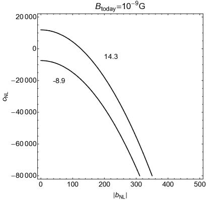
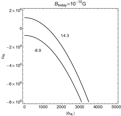
Figure 1: The induced non-Gaussianity parameter $f_{\rm NL}^{\zeta\zeta\zeta_{B}}$ as a function of $b_{\rm NL}$ and $c_{\rm NL}$. The regime compatible with the non-detection by Planck lies between the contours $f_{\rm NL}=-8.9$ and $f_{\rm NL}=14.3$, bounding the Planck $2\sigma$ for $f_{\rm NL}$. The left panel corresponds to situation $B_{\rm today}=10^{-9}$ G marginally allowed by observations and corresponding to ${\cal P}_{\zeta_{B}}\sim{\cal P}_{\zeta}$ and the right panel depicts the case for $B_{\rm today}=10^{-10}$ G where the magnetic contribution to curvature perturbations is subdominant. Here we have set the inflationary slow roll parameter $\epsilon=0.01$.

If the magnetic field amplitude is close to the observational upper bound $B_{\rm today}\sim 10^{-9}$ G one obtains a tight constraint $|b_{\rm NL}|~{}\mbox{\raisebox{-2.58334pt}{$\stackrel{{\scriptstyle<}}{{\sim}}$}}~{}10^{2}$, barring cancellations against the parameter $c_{\rm NL}$. In this case the magnetic contribution to the amplitude of curvature perturbations (4.22) is also non-negligible. For smaller magnetic field amplitudes the bounds on $b_{\rm NL}$ and $c_{\rm NL}$ get relaxed as the the induced non-Gaussianity (4.25) scales as $f_{\rm NL}^{\zeta\zeta\zeta_{B}}\propto B^{2}$.

In a similar way, in the flat case and squeezed limit the induced non-linearity parameter of type $f_{\rm NL}^{\zeta\zeta_{B}\zeta_{B}}$ (4.1) takes the form

$$f_{\rm NL}^{\zeta\zeta_{B}\zeta_{B}}\simeq 0.2b_{\rm NL}\left(\frac{B_{\rm today}}{10^{-9}{\rm G}}\right)^{2}\left(\frac{0.01}{\epsilon}\right)^{2}\left(\frac{N_{\rm CMB}}{N_{0}}\right)^{2}(N_{0}-N_{\rm CMB})\ .$$ (4.26)

Here we have used that ${\cal P}_{\zeta}=2.44\times 10^{-9}$ [59] and $\Omega_{B}\sim 10^{-7}B^{2}_{\rm today}{\rm nG}^{-2}$. Comparing with the result (4.25) we find that the induced non-Gaussianity of type $f_{\rm NL}^{\zeta\zeta_{B}\zeta_{B}}$ generically yields a stronger constraint on $b_{\rm NL}$ but the result depends on the duration of the epoch when magnetic fields were generated. Setting conservatively $N_{0}-N_{\rm CMB}=5$ and choosing $N_{\rm CMB}=60$ one obtains the constraints depicted in Figure 2.

Figure 2: The induced non-Gaussianity parameter $f_{\rm NL}^{\zeta\zeta_{B}\zeta_{B}}$ as a function of $b_{\rm NL}$ and $B_{\rm today}$. The regime compatible with the non-detection by Planck lies below the contours $f_{\rm NL}=-8.9$ and $f_{\rm NL}=14.3$, corresponding to the $2\sigma$ region for $f_{\rm NL}$. Here we have set the inflationary slow roll parameter $\epsilon=0.01$ and assumed the magnetic field generation started $5$ e-foldings before the horizon exit of largest observable modes.

We reiterate that our result assumes the generation of magnetic fields started at some time $t_{0}$ corresponding to the horizon scale $k_{0}=a_{0}H_{0}$ and we assume this was before the horizon crossing of largest observable modes $t_{0}<t_{\rm CMB}$. Formally we are then studying the statistics of fluctuations in a patch of size $k_{0}^{-1}$ which does not in general correspond to the statistics which can be measured in the observable patch of size $k_{\rm CMB}^{-1}<k_{0}^{-1}$, see [61, 62, 63, 64, 65, 66, 67, 68, 69]. If $k_{0}\ll k_{\rm CMB}$ the long-wavelength fluctuations of magnetic fields generate an effective background field for our patch and we should instead consider the statistics of fluctuations around this background. In order to avoid these complications here, we restrict to the case where $N_{0}-N_{\rm CMB}~{}\mbox{\raisebox{-2.58334pt}{$\stackrel{{\scriptstyle<}}{{\sim}}$}}~{}{\cal O}(10)$ so that difference of the statistics of fluctuations in the patches $k_{0}^{-1}$ and $k_{\rm CMB}^{-1}$ is small unless the curvature perturbation would be highly non-Gaussian [65]. This approach remains valid even if the generation of magnetic fields would have started long before the horizon exit of our observable modes but then implicitly assumes that patch $k_{0}^{-1}$ occupies a region where the effective background magnetic field vanishes.

5 Benchmark model

In order to estimate the natural values for $b_{NL}$ and $c_{NL}$, we consider the non-Gaussianities generated by amplification of magnetic fields during inflation in a specific model. We assume the Lagrangian is of the form

$${\cal L}=\frac{1}{2}R-\frac{1}{2}\partial^{\mu}\phi\partial_{\mu}\phi-V(\phi)-\frac{1}{4}\lambda(\phi)F_{\mu\nu}F^{\mu\nu}\ ,$$ (5.1)

where $\lambda(\phi)$ takes a power law form [26, 27, 28, 29, 30, 31, 32]

$$\lambda=\lambda_{I}\left(\frac{a}{a_{I}}\right)^{2n}\ ,$$ (5.2)

and $a_{I}$ denotes the end of inflation. We assume $\phi$ is a slowly rolling scalar field and consider fluctuations around the homogeneous FRW background solution,

$$\bar{\phi}=\bar{\phi}(t)\ ,\qquad{\bar{A}}_{\mu}=0\ .$$ (5.3)

We concentrate on the exponent values $n>-1/2$ for which the large scale modes of the vector potential $A_{i}\sim a^{n}/\lambda^{1/2}$ are nearly constant and the backreaction of the magnetic fields to the inflationary dynamics can be kept small. But as already mentioned, the results in the other regime can be obtained by use of the electromagnetic duality, which leaves the result invariant under a simultaneous exchange of the electric and magnetic field and $n\to-n$ [54, 55, 56].

The electromagnetic part of the action for perturbations is quadratic in $A_{\mu}$, the fluctuation of the vector potential around the zero background, including terms schematically of the form

$${\cal L}_{\rm pert.}\supset A^{2}\zeta^{m}\ .$$ (5.4)

Here $\zeta$ is the curvature perturbation and $m$ is a positive integer. In the Coulomb gauge the magnetic field is related to the vector potential as $B_{i}=a^{-2}\epsilon_{ijk}\partial_{j}A_{k}$.

On superhorizon scales $k\ll aH$, and treating the Hubble rate during inflation as a constant $H=H_{I}$, the spectrum of the magnetic fields generated during inflation then takes the form

$$P_{{\rm B}}(\eta,k)=\frac{4^{n}\Gamma^{2}(n+1/2)}{\lambda(\eta)\pi}\frac{H_{I}^{4}}{k^{3}}(-k\eta)^{4-2n}\ .$$ (5.5)

Due to the fact that the vector potential is approximately constant, the energy density of the electromagnetic field is dominated by the magnetic part

$$\langle\rho_{B}(\eta)\rangle = \frac{\lambda}{2a^{4}}\langle((\partial_{i}A_{j}(t,{\bf x}))(\partial_{i}A_{j}(t,{\bf x}))\rangle$$ (5.6)

$$= \frac{1}{2}\int\frac{dq^{3}}{(2\pi)^{3}}P_{B}(\eta,q)\theta(q-k_{0})\theta(-1/\eta-q)$$ (5.7)

$$= \frac{4^{n-1}\Gamma^{2}(n+1/2)H_{I}^{4}}{\pi^{3}(4-2n)}\left(1-e^{(2n-4)N_{0}}\right)\ .$$ (5.8)

Here $k_{0}$ corresponds to the largest scale at which inflationary magnetic fields are generated. The contribution of the magnetic fields to the total energy density during inflation is then controlled by

$$\frac{\langle\rho_{B}(\eta)\rangle}{\rho_{\rm tot.}}=r_{T}{\cal P}_{\zeta}\frac{4^{n-1}\Gamma^{2}(n+1/2)}{6\pi(4-2n)}\left(1-e^{(2n-4)N_{0}}\right)\ ,$$ (5.9)

where $r_{T}=16\epsilon~{}\mbox{\raisebox{-2.58334pt}{$\stackrel{{\scriptstyle<}}{{\sim}}$}}~{}0.02$ is the tensor to scalar ratio. Using that ${\cal P}_{\zeta}=2.4\times 10^{-9}$ and requiring that the magnetic fields remain subdominant for at least a period of 60 e-foldings one obtains the constraint $n~{}\mbox{\raisebox{-2.58334pt}{$\stackrel{{\scriptstyle<}}{{\sim}}$}}~{}2.2$ [42, 43], unless the scale of inflation is very low [43].

The energy density of the magnetic fields sources the generation of adiabatic curvature perturbation according to the formula (4.1). As the magnetic spectrum (5.5) is of the form (3.3) the spectrum of induced curvature perturbation $\zeta_{B}$ is directly obtained from equation (4) by substituting the corresponding value of $C_{B}$. This yields the result

$${\cal P}_{\zeta_{B}}(\eta,k) \simeq {\cal P}_{\zeta}^{2}\left(\frac{4^{n+1}\Gamma^{2}(n+1/2)}{6\pi}\right)^{2}\times$$

$$\left[\rule{0.0pt}{17.22217pt}\right.\left(C_{1}(n,k)+C_{2}(n,k)e^{(2n-4)(N_{0}-N_{\rm CMB}}\right)\left(\frac{1-e^{(2n-4)N_{\rm CMB}}}{4-2n}\right)^{2}$$

$$+2C_{3}(n,k)\left(\frac{1}{3(4-2n)}-\frac{1}{(4-2n)(2n-1)}e^{(2n-4)N_{\rm CMB}}+\frac{1}{3(2n-1)}e^{3N_{\rm CMB}}\right)\left]\rule{0.0pt}{17.22217pt}\right.\ ,$$

where the coefficients $C_{i}$ are given by equation (3.15).

In the limit of a flat spectrum for the magnetic fields, $n=2$, the leading part of the result takes the simple logarithmic form

$${\cal P}_{\zeta_{B}}^{n=2}(\eta,k)=192\,{\cal P}_{\zeta}^{2}N_{\rm CMB}^{2}(N_{0}-N_{\rm CMB})\ .$$ (5.11)

in agreement with [44]. For a discussion of this apparently coincidental agreement, see appendix A.

Similarly, the $b_{NL}$ dependent contribution to the power spectrum gives in the flat limit

$${\cal P}_{\zeta_{B}}^{(b_{NL})n=2}(\eta,k)=3\,b_{NL}\,{\cal P}_{\zeta}^{2}N_{0}^{2}\ .$$ (5.12)

We notice that for moderate values of $b_{NL}$, the new contribution to the power spectrum (5.12) is the dominant one, although in the local approximation where $b_{NL}=-4$, the contribution (5.11) is larger.

5.1 Induced bispectrum $\langle\zeta_{0}\zeta_{0}\zeta_{B}\rangle$

In the squeezed limit the amplitude of the correlator $\langle\zeta_{0}\zeta_{0}\zeta_{B}\rangle$ can be directly obtained from equation (4.1) using the value of $C_{B}$ obtained by comparing the expressions (3.3) and (5.5). This yields the result

$$f_{\rm NL}^{\zeta\zeta\zeta_{B}} = -20n^{2}{\cal P}_{\zeta}\frac{4^{n+1}\Gamma^{2}(n+1/2)}{18\pi}\times$$

$$\frac{k^{3}_{3}}{4-2n}\left(N_{3}+\frac{e^{(2n-4)N_{0}}}{4-2n}\left(1-e^{-(2n-4)N_{3}}\right)+2{\rm p.}\right)\times\left(k_{1}^{3}+k_{2}^{3}+k_{3}^{3}\right)^{-1}\ .$$

The non-detection of primordial bispectrum by Planck translates into constraints on the parameters $b_{\rm NL}$ and $c_{\rm NL}$. Their values for the benchmark model have been computed in appendix B. In the limit of a flat spectrum of the magnetic fields $n=2$, the induced bispectrum (4.1) takes a local shape and the momentum dependence of the induced $f_{\rm NL}$ vanishes

$$f_{\rm NL}^{\zeta\zeta\zeta_{B},n=2}=-80{\cal P}_{\zeta}N_{0}^{2}\ .$$ (5.14)

Thus, in the local approximation the induced bispectrum from $\left<\zeta\zeta B^{2}\right>$ is well within the observational limits $-8.9<f_{\rm NL}^{\rm local}<14.3$ (95% C.L.) [2] for reasonable values of $N_{0}$.

5.2 Induced bispectrum $\langle\zeta_{0}\zeta_{B}\zeta_{B}\rangle$

In a similar way, substituting the $C_{B}$ obtained from (3.3) and (5.5) into equation (4.1) we find that the non-linearity parameter induced by the cross correlator $\langle\zeta_{0}\zeta_{B}\zeta_{B}\rangle$ in the squeezed limit $k_{1}\ll k_{2}\sim k_{3}$ is given by

$$f_{\rm NL}^{\zeta\zeta_{B}\zeta_{B}} = -\frac{10}{6}n{\cal P}_{\zeta}\left(\frac{4^{n+1}\Gamma^{2}(n+1/2)}{6\pi}\right)^{2}\times$$ (5.15)

$$\left[\rule{0.0pt}{17.22217pt}\right.k_{3}^{3}\left(C_{1}(n)+C_{2}(n)e^{(2n-4)(N_{0}-N_{2})}\right)e^{(2n-4)(N_{2}-N_{3}))}\left(\frac{(1-e^{(2n-1)N_{2}})(1-e^{(2n-1)N_{3}})}{(4-2n)^{2}}\right)$$

$$+C_{3}(n)k_{3}^{3}\left(1+e^{(2n-1)(N_{3}-N_{2})}\rule{0.0pt}{12.91663pt}\right.\left)\rule{0.0pt}{12.91663pt}\right.\frac{1}{(2n-1)(4-2n)}\left(\rule{0.0pt}{12.91663pt}\right.1-e^{(2n-4)N_{2}}\left)\rule{0.0pt}{12.91663pt}\right.$$

$$+C_{3}(n)\frac{2k_{3}^{3}}{3(2n-1)}(1+e^{-3N_{2}})+5{\rm p.}\left]\rule{0.0pt}{17.22217pt}\right.\times\left[k_{1}^{3}+k_{2}^{3}+k_{3}^{3}\right]^{-1}\ .$$

For the special case of a flat spectrum $n=2$ for magnetic fields, the result takes the form

$$f_{\rm NL}^{\zeta\zeta_{B}\zeta_{B},n=2}=-640\,{\cal P}_{\zeta}\left(\frac{k_{3}^{3}N_{3}N_{2}(N_{0}-N_{2})+5{\rm p.}}{k_{1}^{3}+k_{2}^{3}+k_{3}^{3}}\right)\ .$$ (5.16)

Using that within the squeezed limit approximation $k_{1}\ll k_{2}\sim k_{3}$ and using ${\cal P}_{\zeta}=2.4\times 10^{-9}$ we get the result

$$f_{\rm NL}^{\zeta\zeta_{B}\zeta_{B},n=2}\sim-16\times 10^{-7}\,N_{2}\left(N_{2}(N_{0}-N_{1})+N_{1}(N_{0}-N_{2})\right)\ .$$ (5.17)

which is also within observational bounds for reasonable values of $N_{0}$, $N_{1}$ and $N_{2}$

Folded shape

Another important shape is the flattened limit $k_{1}=2k_{2}=2k_{3}$, where it was earlier found that the magnetic non-linearity parameter, $b_{NL}$, can be large. It was calculated in [50] that $b_{NL}\sim 5760$ in this shape, and the dominating contribution to the cross-correlation function comes from

$$A\approx\hat{p}\cdot\hat{r}\frac{k_{1}^{3}}{(pr)^{3/2}}3(n_{B}-4)\log(-(k_{1}+p+r)\tau_{I})~{},$$ (5.18)

$$D\approx-\frac{k_{1}^{3}}{(pr)^{3/2}}3(n_{B}-4)\log(-(k_{1}+p+r)\tau_{I})~{},\qquad J=0,$$

as discussed in appendix C.

With this ansatz, we can carry out the angular integrals in the flattened limit $k_{1}=2k_{2}=2k_{3}$ in the scale invariant case. The angular integrals then gives the leading contribution

$$\langle\zeta_{0}({\bf k}_{1}){\bf B}^{2}({\bf k}_{2}){\bf B}^{2}({\bf k}_{3})\rangle_{\rm c} = 20(2\pi)^{3}\delta({\bf k}_{1}+{\bf k}_{2}+{\bf k}_{3})P_{\zeta}(k_{1})P_{{\rm B}}(k_{2})\left(\frac{k_{1}}{k_{3}}\right)^{3}{\mathcal{P}_{\zeta}}$$

$$\times\frac{3H^{4}}{4\pi^{2}\lambda}3(n_{B}-4)(N_{0}-N_{\rm CMB})$$

from which we can obtain

$$\langle\zeta_{0}({\bf k}_{1}){\zeta_{B}}({\bf k}_{2}){\zeta_{B}}({\bf k}_{3})\rangle = (2\pi)^{3}\delta({\bf k}_{1}+{\bf k}_{2}+{\bf k}_{3})P_{\zeta}(k_{1})P_{\zeta}(k_{2})\left(\frac{k_{1}}{k_{3}}\right)^{3}\frac{\mathcal{P_{\zeta_{B}}}}{\mathcal{P}_{\zeta}}$$

$$\times-\frac{15}{2}(n_{B}-4)(N_{0}-N_{\rm CMB})$$

If we insert the expression for $\mathcal{P_{\zeta_{B}}}$, we obtain

$$|f_{\rm NL}^{flat~{}(\zeta\zeta_{B}\zeta_{B})}|\sim 11520{\cal P}_{\zeta}N_{\rm CMB}^{2}\,(N_{0}-N_{\rm CMB})^{2}\ .$$ (5.21)

Taking $P_{\zeta}=2.4\times 10^{-9}$ and $N_{CMB}=60$, we note that $N_{0}=70$ already induces large non-Gaussianity.

5.3 Induced bispectrum $\langle\zeta_{B}\zeta_{B}\zeta_{B}\rangle$

The integral in (4.1) can be evaluated using the magnetic spectrum (5.5) which gives the time evolution of the magnetic fields on superhorizon scales. For $n>1/2$ and for momentum configurations with $k_{i}\sim k$, the induced three point function is given by [46]

$$\langle\zeta_{B}({\bf k}_{1})\zeta_{B}({\bf k}_{2})\zeta_{B}({\bf k}_{3})\rangle_{\rm c} \simeq (2\pi)^{3}\delta({\bf k}_{1}+{\bf k}_{2}+{\bf k}_{3})P_{\zeta}(k_{1})P_{\zeta}(k_{2}){\cal P}_{\zeta}\left(\frac{4^{n+1}\Gamma^{2}(n+1/2)}{3\pi}\right)^{3}$$

$$\frac{2+2{\rm cos}^{2}({\bf k}_{1},{\bf k}_{2})}{3(4-2n)^{4}}\left(1-e^{(4-2n)(N_{\rm CMB}-N_{0})}\right)\left(e^{-(4-2n)N_{\rm CMB}}-1\right)^{3}+2{\rm p}.$$

The corresponding contribution to the non-linearity parameter $f_{\rm NL}$ reads

$$f_{\rm NL}^{\zeta_{B}\zeta_{B}\zeta_{B}} \simeq {\cal P}_{\zeta}\left(\frac{4^{n+1}\Gamma^{2}(n+1/2)}{3\pi}\right)^{3}\frac{5}{9(4-2n)^{4}}\left(1-e^{(4-2n)(N_{\rm CMB}-N_{0})}\right)\left(e^{-(4-2n)N_{\rm CMB}}-1\right)^{3}\times$$ (5.23)

$$\frac{k_{3}^{3}(1+{\rm cos}^{2}({\bf k}_{1},{\bf k}_{2}))+2{\rm p.}}{k_{1}^{3}+k_{2}^{3}+k_{3}^{3}}\ .$$

In the limit of a flat spectrum for magnetic fields $n=2$ and for the folded shape $\bm{\mathrm{{k}}}\equiv\bm{\mathrm{{k}}}_{1}=-2\bm{\mathrm{{k}}}_{2}=-2\bm{\mathrm{{k}}}_{3}$, we then obtain

$$|f_{\rm NL}^{\zeta_{B}\zeta_{B}\zeta_{B},n=2}|=1536{\cal P}_{\zeta}N_{\rm CMB}^{3}(N_{0}-N_{\rm CMB})\ .$$ (5.24)

which is shown in the rightmost panel of Figure 3 and Figure 4 and compared with $f_{\rm NL}^{\zeta\zeta_{B}\zeta_{B},n=2}$ in (5.21) shown in the leftmost panel of Figure 3 and Figure 4.

Figure 3: The induced $|f_{NL}|$ as a function of the scale $N_{k}=\ln(k/a_{0}H_{0})$ in the case where the total number of e-folds is $N_{total}=60$. The left panel is $|f_{NL}^{\zeta\zeta_{B}\zeta_{B}}|$ and the right panel is $|f_{NL}^{\zeta_{B}\zeta_{B}\zeta_{B}}|$.

Figure 4: The induced $|f_{NL}|$ as a function of the scale $N_{k}=\ln(k/a_{0}H_{0})$ in the case where the total number of e-folds is $N_{total}=70$. The left panel is $|f_{NL}^{\zeta\zeta_{B}\zeta_{B}}|$ and the right panel is $|f_{NL}^{\zeta_{B}\zeta_{B}\zeta_{B}}|$

We see that for very moderate amount of total inflation, slightly more that the required $60$ e-folds, the new non-Gaussian contribution to the CMB from $f_{\rm NL}^{\zeta\zeta_{B}\zeta_{B},n=2}$ in (5.21) can be very large on CMB scales, and potentially provide very strong constraints on the model.

6 Summary and conclusions

We have studied the constraints on gauge field production during inflation imposed by requiring that their effect on the CMB anisotropies are subdominant. Focussing on the non-Gaussianity induced by the gauge field production, we studied for the first time the bispectrum of the primordial curvature perturbation induced by the cross correlation between the curvature perturbation induced by the inflaton and the curvature perturbation induced by the magnetic field, defined by the gauge field. In order to make this study as model-independent as possible, we used a general parametrization of the cross correlation between the magnetic field, and the primordial curvature perturbation in terms of the magnetic non-linearity parameters. In order to facilitate this parametrization, we have defined the magnetic non-linearity parameters $\beta_{NL}$, $c_{NL}$ characterizing the strength of the four point function $\left<\zeta_{0}\zeta_{0}B^{2}\right>$, in addition to the non-linearity parameter $b_{NL}$ parametrizing the strength of the three-point cross-correlation function $\left<\zeta_{0}B^{2}\right>$. In appendix B the non-linearity p! arameters were computed in the squeezed limit.

Since the magnetic field squared $B^{2}$ acts as a non-Gaussian iso-curvature perturbation during inflation, it induces a non-Gaussian primordial curvature perturbation $\zeta_{B}$. As a measure of this non-Gaussianity, we have computed the induced primordial curvature bispectrum from the contributions of the form $\left<\zeta_{0}\zeta_{0}\zeta_{B}\right>$, $\left<\zeta_{0}\zeta_{B}\zeta_{B}\right>$ and $\left<\zeta_{B}\zeta_{B}\zeta_{B}\right>$. The first two of these depend on $b_{NL}$ and $c_{NL}$ and can be used to derive observational constrains on the magnetic non-linearity parameters. Assuming a power law parametrization for the spectrum of the magnetic fields produced during inflation but treating the coupling $\lambda(\phi)$ as a free function, we have then derived the observational constraints on $b_{NL}$ and $c_{NL}$.

In particular we have shown that in a general class of models, the new contribution to the bispectrum of the primordial curvature perturbation from $\left<\zeta_{0}\zeta_{B}\zeta_{B}\right>$ can be the dominant source of non-Gaussianity and lead to a large non-Gaussian contribution in the folded shape if inflation last only slightly longer than the required $60$ e-folds. This implies new strong phenomenological constraints on gauge field production in this class of models when compared with the absence of a non-Gaussian primordial signal as observed by the Planck satellite [2].

If inflation last much longer than the observable $60$ e-folds, the results presented here will provide the average correlation function in the full inflated volume, while the observed correlation function may deviate from this value [61, 62, 63, 64, 65, 66, 67, 68, 69, 70]. In this case, one should treat the long wavelength modes as a homogenous background for the shorter wavelength modes within the observable region, which by its vector nature breaks isotropy. In that case effects similar to those discussed here leads to further new constraints on the magnetic non-linearity parameters by their anisotopic contribution to the power spectrum and bispectrum of the curvature perturbation. The analogous $b_{NL}$ independent effects was discussed in [71] (see also [72, 73, 74, 75]). While it is beyond the scope of the present work, it would be interesting in the future to study also the new sources of anisotropy from the cross correlation functions of the magnetic field with the inflaton.

Acknowledgments: SN is supported by the Academy of Finland grant 257532 and MSS is support by a Lundbeck Foundation Jr. Group Leader Fellowship.

Appendix A Source term in the scale-invariant limit

From the definition of the curvature perturbation in terms of the inflaton and gauge field curvature perturbations

$$\zeta=\zeta_{\phi}+\tilde{\zeta}_{B}$$ (A.1)

we have the equations governing their time-evolution derived in (1) in the introduction

$$\dot{\zeta}_{\phi}=H\frac{Q}{\dot{\rho}}~{},\qquad\dot{\tilde{\zeta}}_{B}=-H\frac{Q}{\dot{\rho}}-\frac{H}{\rho+p}\delta P_{nad}$$ (A.2)

where

$$\delta P_{nad}=\delta p_{B}-\frac{\dot{p}}{\dot{\rho}}\delta\rho_{B}=\frac{4}{3}\delta\rho_{B}~{}.$$ (A.3)

It follows from (A.1) and (A.2) that only if

$$H\frac{Q}{\dot{\rho}}=-\frac{H}{\rho+p}\delta P_{nad}~{},$$ (A.4)

it is consistent to assume

$$\dot{\zeta}=\dot{\zeta}_{\phi}+\dot{\tilde{\zeta}}_{B}\approx\dot{\zeta}_{\phi}=H\frac{Q}{\dot{\rho}}~{},$$ (A.5)

like in [44, 45], instead of using the more generally valid expression

$$\dot{\zeta}=-\frac{H}{\rho+p}\delta P_{nad}~{}.$$ (A.6)

Since the source term, $Q$, is given by

$$Q=\frac{\dot{\lambda}}{\lambda}\delta\rho_{B}$$ (A.7)

then with the assumption of a power-law behavior $\lambda=\lambda_{0}(a/a_{0})^{2n}$, such that $\dot{\lambda}/\lambda=2nH$, we have that the condition (A.4) for the approximations in [44, 45] to be valid, becomes equivalent the the condition

$$2n\frac{H^{2}}{\dot{\rho}}\delta\rho_{B}=-\frac{4}{3}\frac{H}{\rho+p}\delta\rho_{B}$$ (A.8)

where we used (A.3). Now using that $\dot{\rho}=-3(\rho+p)$, we have that this condition is only satisfied in the flat case when $n=2$. This explains why [44, 45] finds the right spectrum $P_{\zeta_{B}}$ in the flat limit, even if their treatment is generally formally inconsistent.

Appendix B Parametrization of $P_{B}(k)$ and local magnetic non-linearity parameters

We briefly review the magnetic consistency relation for $b_{NL}^{local}$ [49], and generalize it to $c_{NL}^{local}$.

Let us consider the basic correlation function $\left<\zeta_{0}(\tau_{I},\bm{\mathrm{{k}}}_{1})A_{i}(\tau_{I},\bm{\mathrm{{k}}}_{2})A_{j}(\tau_{I},\bm{\mathrm{{k}}}_{3})\right>$ in the squeezed limit $k_{1}\ll k_{2},k_{3}$. In this limit, the only effect of the long wavelength mode $\zeta_{0}(\tau,\bm{\mathrm{{k}}}_{1})$ is to locally rescale the background as $a\to a_{B}=e^{\zeta_{B}}a$ when computing the correlation functions on shorter scales given by $k_{2},k_{3}$, and one can therefore as usual write

$$\lim_{k_{1},\dots,k_{n}\to 0}\left<\zeta_{0}(\tau_{I},\bm{\mathrm{{k}}}_{1})\dots\zeta_{0}(\tau_{I},\bm{\mathrm{{k}}}_{n})A_{i}(\tau_{I},\bm{\mathrm{{k}}}_{n+1})A_{j}(\tau_{I},\bm{\mathrm{{k}}}_{n+2})\right>$$

$$\qquad=\left<\zeta_{0}(\tau_{I},\bm{\mathrm{{k}}}_{1})\dots\zeta_{0}(\tau_{I},\bm{\mathrm{{k}}}_{n})\left<A_{i}(\tau_{I},\bm{\mathrm{{k}}}_{n+1})A_{j}(\tau_{I},\bm{\mathrm{{k}}}_{n+2})\right>_{\zeta_{0}}\right>.$$ (B.1)

Here $\left<A_{i}(\tau_{I},\bm{\mathrm{{k}}}_{2})A_{j}(\tau_{I},\bm{\mathrm{{k}}}_{3})\right>_{\zeta_{0}}$ is the correlation function of the short wavelength modes in the background of the long wavelength modes of $\zeta_{0}$ .

Since the equations of motion of the gauge field are conformal invariant in the absence of the coupling $\lambda(\phi)$, it follows that the gauge field only feels the background expansion through the coupling $\lambda$, where $\lambda$ depends on the scale factor through $\phi$. Using that the gauge field scales like $1/\sqrt{\lambda}$, then in order to evaluate the correlation function for a non-trivial $\lambda$, one can then write $A_{i}(\tau,\bm{\mathrm{{k}}})$ in terms of the Gaussian field $A_{i}(\tau,\bm{\mathrm{{k}}})=\sqrt{(\lambda_{0}/\lambda)}A_{i}^{(G)}(\tau,\bm{\mathrm{{k}}})$, where the Gaussian gauge field $A_{i}^{(G)}(\tau,\bm{\mathrm{{k}}})$ is defined with a homogeneous background coupling, $\lambda_{0}$, and then expand $\lambda=\lambda(a)$ around the homogenous background value,

$$\lambda=\lambda_{0}+\frac{d\lambda_{0}}{d\ln a}\delta\ln a+\frac{1}{2}\frac{d^{2}\lambda_{0}}{d\ln a^{2}}\delta\ln a^{2}+\dots=\lambda_{0}+\frac{d\lambda_{0}}{d\ln a}\zeta_{0}+\frac{1}{2}\frac{d^{2}\lambda_{0}}{d\ln a^{2}}\zeta_{0}^{2}+\dots~{}.$$ (B.2)

which yields

$$A_{i}(\tau,\bm{\mathrm{{k}}})=A_{i}^{(G)}(\tau,\bm{\mathrm{{k}}})\left(1-\frac{1}{2}\frac{1}{H}\frac{\dot{\lambda}}{\lambda}\zeta_{0}+\left(\frac{3}{8}\frac{1}{H^{2}}\frac{\dot{\lambda}^{2}}{\lambda^{2}}-\frac{1}{4}\frac{1}{H^{2}}\frac{\ddot{\lambda}}{\lambda}\right)\zeta_{0}^{2}+\dots\right)$$ (B.3)

By comparison with the definitions of $b_{NL}$ and $c_{NL}$ in equation (2.7), we conclude that

$$b_{NL}=-\frac{1}{H}\frac{\dot{\lambda}}{\lambda}$$ (B.4)

and

$$c_{NL}=\frac{9}{4}\frac{1}{H^{2}}\frac{\dot{\lambda}^{2}}{\lambda^{2}}-\frac{3}{2}\frac{1}{H^{2}}\frac{\ddot{\lambda}}{\lambda}~{}.$$ (B.5)

Finally by inserting the expansion (B.3) into (B), we can reproduce the consistency relations

$$\lim_{k_{1}\to 0}\left<\zeta_{0}(\tau_{I},\bm{\mathrm{{k}}}_{1}){\bf B}(\tau_{I},\bm{\mathrm{{k}}}_{2})\cdot{\bf B}(\tau_{I},\bm{\mathrm{{k}}}_{3})\right>$$

$$\qquad=-\frac{1}{H}\frac{\dot{\lambda}}{\lambda}(2\pi)^{3}\delta^{(3)}(\bm{\mathrm{{k}}}_{1}+\bm{\mathrm{{k}}}_{2}+\bm{\mathrm{{k}}}_{3})P_{\zeta}(k_{1})P_{B}(k_{2})$$ (B.6)

and

$$\lim_{k_{1},k_{2}\to 0}\left<\zeta(\tau_{I},\bm{\mathrm{{k}}}_{1})\zeta_{0}(\tau_{I},\bm{\mathrm{{k}}}_{2}){\bf B}(\tau_{I},\bm{\mathrm{{k}}}_{3})\cdot{\bf B}(\tau_{I},\bm{\mathrm{{k}}}_{4})\right>$$

$$\qquad=\left(2\frac{1}{H^{2}}\frac{\dot{\lambda}^{2}}{\lambda^{2}}-\frac{1}{H^{2}}\frac{\ddot{\lambda}}{\lambda}\right)(2\pi)^{3}\delta^{(3)}(\bm{\mathrm{{k}}}_{1}+\bm{\mathrm{{k}}}_{2}+\bm{\mathrm{{k}}}_{3}+\bm{\mathrm{{k}}}_{4})P_{\zeta}(k_{1})P_{\zeta}(k_{2})P_{B}(k_{3})$$ (B.7)

Using the power-law assumption for the coupling in terms of the scale-factor, $\lambda\propto a^{2n}(t)$, when then obtain from (B.4) and (B.5)

$$b_{NL}=-2n=n_{B}-4~{},\qquad c_{NL}=\frac{3}{4}b_{NL}^{2}\ .$$ (B.8)

Therefore, in this case the magnetic non-linearity parameters are fully determined by the exponent. The magnetic spectrum also takes a power law form $P_{B}\propto k^{1-2n}$ as can be seen in its explicit expression (5.5).

In most of the paper we have for simplicity assumed the magnetic spectrum, $P_{B}(k)$, to have a power law form. If this is derived from assuming that the coupling, $\lambda$, also have the simple power law form, then we have just seen how $b_{NL}$ and $c_{NL}$ are fixed the power law index $n$. If the power law assumption for $\lambda$ was the only way to obtain a power law form for the magnetic spectrum, $P_{B}(k)$, it would therefore not make much sense to constrain $b_{NL}$ and $c_{NL}$ in a model independent way. Here we will therefore demonstrate with a concrete example that a power law spectrum $P_{B}$ (3.3) can be generated also for more general couplings $\lambda(a)$ which are not of the simple power law form. In this case the magnetic non-linearity parameters $b_{\rm NL}$ and $c_{\rm NL}$ are in general independent of each other and their magnitudes are not determined by the properties of the spectrum.

We work in the Coulomb gauge specified by the conditions $A_{0}=0$ and $\partial_{i}A_{i}=0$. The spatial part of the vector potential is then decomposed in the standard way

$$A^{i}_{{\bf k}}=\sum_{\sigma=\pm}\left(\epsilon_{\sigma}^{i}({\bf k})e^{i{\bf k}\cdot{\bf x}}\hat{a}_{\sigma}({\bf k})A_{{\bf k}}+h.c.\right)\ ,$$ (B.9)

where the polarization operators satisfy $k_{i}\epsilon_{i}^{\sigma}=0,~{}\epsilon_{i}^{\sigma}{\epsilon_{i}^{\sigma^{\prime}}}^{*}=\delta^{\sigma\sigma^{\prime}},~{}\epsilon_{i}^{\sigma}{\epsilon_{j}^{\sigma}}^{*}=\delta_{ij}-k_{i}k_{j}/k^{2}$. The commutation relations of the creation /annihilation operators are given by $[\hat{a}^{\sigma}_{{\bf k}},\hat{a}^{\sigma^{\prime}}_{{\bf k}^{\prime}}{}^{{\dagger}}]=(2\pi)^{2}\delta({\bf k}-{\bf k}^{\prime})\delta^{\sigma\sigma^{\prime}}$. The equation of motion is then given by

$$(\sqrt{\lambda}A_{{\bf k}})^{\prime\prime}+\left(k^{2}-\frac{(\sqrt{\lambda})^{\prime\prime}}{\sqrt{\lambda}}\right)\sqrt{\lambda}A_{{\bf k}}=0\ ,$$ (B.10)

where the prime denotes a derivative with respect to the conformal time $\eta=-1/(aH)$. In the superhorizon limit $k\ll-1/\eta$ the gradient term in (B.10) can be neglected and the equation of motion recast in the simple form

$$(\lambda A^{\prime}_{{\bf k}})^{\prime}=0\ .$$ (B.11)

Using the definitions above we can expand the coupling $\lambda(a)$ as

$$\lambda(a)=\lambda_{0}\left(1-b_{\rm NL}{\rm ln}\frac{a}{a_{0}}+\left(\frac{3}{4}b_{\rm NL}^{2}-\frac{1}{3}c_{\rm NL}\right){\rm ln}^{2}\frac{a}{a_{0}}+\ldots\right)\ .$$ (B.12)

Substituting this into (B.11) we can express the superhorizon solution for the vector potential in the integral form

$$A_{{\bf k}}(a)=\frac{D}{a_{0}H\lambda_{0}}\int\limits_{0}^{{\rm ln}(a/a_{0})}\frac{{\rm d}x}{e^{x}(1-b_{\rm NL}x-(3b_{\rm NL}^{2}/4-c_{\rm NL}/3)x^{2}+\ldots)}\ .$$ (B.13)

where $D$ is a constant to be determined by matching with the subhorizon solution. Setting now $c_{\rm NL}=9b_{\rm NL}^{2}/4$ so that the second order term in (B.12) vanishes, neglecting the higher order corrections denoted by the ellipsis, we obtain the result

$$A_{{\bf k}}(a)=\frac{D}{a_{0}H\lambda_{0}}\frac{e^{1/b_{\rm NL}}}{b_{\rm NL}}\left({\rm Ei}(-1/b_{\rm NL}-{\rm ln}(a/a_{0}))-{\rm Ei}(-1/b_{\rm NL})\right)\ .$$ (B.14)

Here ${\rm Ei}(z)$ denotes the exponential integral ${\rm Ei}(z)=-\int_{-z}^{\infty}{\rm d}te^{-t}/t$. To determine the constant $D$ we match this superhorizon solution with the subhorizon solution $A_{{\bf k}}^{\rm sub}=e^{ik\eta}/\sqrt{k\lambda(\eta)}$ at horizon crossing by setting $|A_{{\bf k}}(a=k/H)|=|A_{{\bf k}}^{\rm sub}(a=k/H)|$. This renders the superhorizon result in the form

$$A_{{\bf k}}(a\gg k/H)=\frac{1}{\sqrt{k\lambda(k/H)}}\frac{{\rm Ei}(-1/b_{\rm NL}-{\rm ln}(a/a_{0}))-{\rm Ei}(-1/b_{\rm NL})}{{\rm Ei}(-1/b_{\rm NL}-{\rm ln}(k/k_{0}))-{\rm Ei}(-1/b_{\rm NL})}\approx\frac{1}{\sqrt{k\lambda(k/H)}}\ ,$$ (B.15)

where the last approximative form holds in the limit $k\gg k_{0}$ and $k_{0}=a_{0}H$. Taking the limit $k\gg k_{0}$ of the superhorizon result implies that $a/a_{0}\gg k/(a_{0}H)\gg 1$. In other words this corresponds considering modes $k$ bigger than the expansion scale $k_{0}$ long after the horizon crossing of the mode $k_{0}$.

Using the asymptotic result for the vector potential $A_{{\bf k}}(a)\approx 1/\sqrt{k\lambda(k/H)}$ we can then work out the corresponding spectrum of magnetic fields. The result is given by

$$P_{B}(\eta,k) = 2\frac{k^{2}}{a^{4}}|A_{{\bf k}}(\eta)|^{2}$$

$$= \frac{2H^{4}}{\lambda(\eta)}\frac{1-b_{\rm NL}{\rm ln}(-k_{0}\eta)}{1-b_{\rm NL}{\rm ln}(k/k_{0})}(-{\bf k}\eta)^{4}k^{-3}$$

$$\approx \frac{2H^{4}}{\lambda(\eta)}(-{\bf k}\eta)^{4-1/{\rm ln}(k/k_{0})}k^{-3}\ ,$$

where in the last step we have used that ${\rm ln}(k/k_{0})\gg 1$. Therefore, in this limit we find that the power spectrum of the magnetic fields is approximatively of the power law form (3.3) even if the coupling is given by $\lambda=\lambda_{0}(1-b_{\rm NL}{\rm ln}(a/a_{0}))$ instead of a power law $\lambda\propto a^{n}$.

As a an explicit toy example it shows, that if we choose the coupling constant to be a constant up to a logarithmic correction, then as expected it reproduce the spectrum with a constant coupling function up to logarithmic corrections, but interestingly now $b_{NL}$ is a free parameter. Although the generated magnetic field at the end of inflation is small in this model, and therefore not of great phenomenological interest, it serves as a useful demonstration model for the purpose of showing that in general $b_{\rm NL}$ and $c_{\rm NL}$ should treated as free parameters in a general treatment.

In fact, as also discussed in the introduction, we might expect that the relation between the form of the coupling, $\lambda$, and the magnetic non-linearity parameters, will be different in models with deviations from the Bunchs-Davis vacuum or with extra degrees of freedom.

Appendix C The tensor structure of the cross-correlation bispectrum

Analogous to (2.1), it is convenient to introduce also a tensor bispectrum, where the magnetic fields are left uncontracted

$$\left<\zeta(\bm{\mathrm{{k}}}_{1})B_{i}(\bm{\mathrm{{k}}}_{2})B_{j}(\bm{\mathrm{{k}}}_{3})\right>\equiv(2\pi)^{3}\delta^{(3)}(\bm{\mathrm{{k}}}_{1}+\bm{\mathrm{{k}}}_{2}+\bm{\mathrm{{k}}}_{3})B_{ij}^{\zeta BB}(\bm{\mathrm{{k}}}_{1},\bm{\mathrm{{k}}}_{2},\bm{\mathrm{{k}}}_{3})~{}.$$ (C.1)

The tensor cross-correlation bispectrum of the curvature perturbation with the magnetic field, is constructed from the more fundamental correlation function of the curvature perturbation with the vector field itself $\left<\zeta(k_{1})A_{i}(k_{2})A_{j}(k_{3})\right>$, which places some constraints on its general form. We will assume that $\left<\zeta(k_{1})A_{i}(k_{2})A_{j}(k_{3})\right>$ is a tensor function of $\hat{k}_{2}$ and $\hat{k}_{3}$

$$\left<\zeta(\bm{\mathrm{{k}}}_{1})A_{i}(\bm{\mathrm{{k}}}_{2})A_{j}(\bm{\mathrm{{k}}}_{3})\right> = (2\pi)^{3}\delta^{(3)}(\bm{\mathrm{{k}}}_{1}+\bm{\mathrm{{k}}}_{2}+\bm{\mathrm{{k}}}_{3})\left[A\delta_{ij}+B(\hat{k}_{2i}\hat{k}_{2j}+\hat{k}_{3i}\hat{k}_{3j})\right.$$ (C.2)

$$+C\hat{k}_{2i}\hat{k}_{3j}+D\hat{k}_{2j}\hat{k}_{3i}+E\hat{k}_{2i}(\hat{k}_{2}\times\hat{k}_{3})_{j}+F\hat{k}_{2j}(\hat{k}_{2}\times\hat{k}_{3})_{i}$$

$$+G\hat{k}_{3i}(\hat{k}_{2}\times\hat{k}_{3})_{j}+H\hat{k}_{3j}(\hat{k}_{2}\times\hat{k}_{3})_{i}$$

$$\left.+J(\hat{k}_{2}\times\hat{k}_{3})_{i}(\hat{k}_{2}\times\hat{k}_{3})_{j})\right]|\zeta_{k_{1}}|^{2}|A_{k_{2}}||A_{k_{3}}|~{}.$$

where $\zeta_{k}$ and $A_{k}$ are the mode functions of the curvature perturbation and the vector field respectively. Using that the correlation function is invariant under the exchange of $A_{i}(k_{2})$ and $A_{j}(k_{3})$, we have $E=F$ and $G=H$, and using

$$\left<\zeta(\bm{\mathrm{{k}}}_{1})B_{i}(\bm{\mathrm{{k}}}_{2})B_{j}(\bm{\mathrm{{k}}}_{3})\right>=\epsilon_{ilk}\epsilon_{jmn}k_{2}^{l}k_{3}^{m}\left<\zeta(\bm{\mathrm{{k}}}_{1})A^{k}(\bm{\mathrm{{k}}}_{2})A^{n}(\bm{\mathrm{{k}}}_{3})\right>~{},$$ (C.3)

we obtain

$$B_{ij}^{\zeta BB} = \left[A(\delta_{ij}\delta_{lm}-\delta_{im}\delta_{lj})\hat{k}_{2l}\hat{k}_{3m}+D(\hat{k}_{2}\times\hat{k}_{3})_{i}(\hat{k}_{2}\times\hat{k}_{3})_{j}\right.$$ (C.4)

$$+G((\hat{k}_{2}\times\hat{k}_{3})_{i}(\hat{k}_{2}-\hat{k}_{3}\hat{k}_{2}\cdot\hat{k}_{3})_{j}-(\hat{k}_{2}\times\hat{k}_{3})_{j}(\hat{k}_{2}-\hat{k}_{3}\hat{k}_{2}\cdot\hat{k}_{3})_{i})$$

$$\left.+J(\hat{k}_{2}\hat{k}_{2}\cdot\hat{k}_{3}-\hat{k}_{3})_{i}(\hat{k}_{2}-\hat{k}_{3}\hat{k}_{2}\cdot\hat{k}_{3})_{j}\right]P_{\zeta}(k_{1})\sqrt{P_{B}(k_{2})P_{B}(k_{3})}~{}.$$

The trace of the magnetic non-linearity parameter $b_{NL}$ is given by the trace of $B_{ij}^{\zeta BB}$,

$$b_{NL}=2\frac{\textrm{Tr}(B^{\zeta BB})}{P_{\zeta}(k_{1})(P_{B}(k_{2})+P_{B}(k_{3}))}~{},$$ (C.5)

where with $\bm{\mathrm{{k}}}_{2}\cdot\bm{\mathrm{{k}}}_{3}=k_{2}k_{3}\cos\theta$, we have

$$\textrm{Tr}(B^{\zeta BB})=(2A\cos\theta+D\sin^{2}\theta+J\sin^{2}\theta\cos\theta)P_{\zeta}(k_{1})\sqrt{P_{B}(k_{2})P_{B}(k_{3})}~{}.$$ (C.6)

In the squeezed limit, we have $\cos\theta=-1$ and in the flattened shape, we have $\cos=1$ and $k_{2}=k_{3}$. Thus in these shapes, we have

$$b_{NL}^{local}=-2A~{},\qquad b_{NL}^{flat}=2A~{}.$$ (C.7)

Another simple shape is the orthogonal shape $\cos\theta=0$, for which we have

$$b_{NL}^{orthogonal}=2D\frac{\sqrt{P_{B}(k_{2})P_{B}(k_{3})}}{P_{B}(k_{2})+P_{B}(k_{3})}~{}.$$ (C.8)

On the other hand the equilateral shape contains contributions from both $A,D$ and $J$.

By noticing the fact that the de Sitter isometries becomes the conformal group on the future boundary of de Sitter space, it has been argued that one can use this conformal symmetry to constrain the asymptotic super horizon structure of the correlation function in $\langle\zeta(\bm{\mathrm{{k}}}_{1})A_{i}(\bm{\mathrm{{k}}}_{2})A_{j}(\bm{\mathrm{{k}}}_{3})\rangle$ in (C.2) [51]. The result of [51] obtained with $n=2$, can be reproduced in the current parametrization in (C.2) by taking $A=-(\hat{k}_{2}\cdot\hat{k}_{3})D$ and $B=C=F=G=H=J=0$. This means that in this case by symmetries alone, we can determine that the leading logarithmical divergent contribution at late time, is given by $A$, $D$ up to an overall numerical factor. The precise calculation of the full correlation function shows that in this case, the dominant term in the limit $\log(-k_{t}\tau)\to\infty$ are

$$A\approx\hat{k}_{2}\cdot\hat{k}_{3}\frac{k_{1}^{3}}{(k_{2}k_{3})^{3/2}}3(n_{B}-4)\log(-k_{t}\tau_{I})~{},\qquad D\approx-\frac{k_{1}^{3}}{(k_{2}k_{3})^{3/2}}3(n_{B}-4)\log(-k_{t}\tau_{I})~{},$$ (C.9)

where $k_{t}=k_{1}+k_{2}+k_{3}$. One important subtlety of this argument is however that these leading logarithmic terms are suppressed by a factor of $k_{1}^{3}$, which vanishes in the exactly squeezed limit $k_{1}\to 0$. Instead, as mention above, in the squeezeed limit we can identify $A$ with $-b_{NL}^{local}/2$, which can be obtained from the squeezed limit magnetic consistency relation [49, 50].

References

• [1] Planck Collaboration Collaboration, P. Ade et al., Planck 2013 results. XXII. Constraints on inflation, arXiv:1303.5082.
• [2] Planck Collaboration Collaboration, P. Ade et al., Planck 2013 Results. XXIV. Constraints on primordial non-Gaussianity, arXiv:1303.5084.
• [3] J. Lesgourgues and S. Pastor, Massive neutrinos and cosmology, Phys.Rept. 429 (2006) 307–379, [astro-ph/0603494].
• [4] S. Hannestad, Neutrino physics from precision cosmology, Prog.Part.Nucl.Phys. 65 (2010) 185–208, [arXiv:1007.0658].
• [5] Y. Y. Wong, Neutrino mass in cosmology: status and prospects, Ann.Rev.Nucl.Part.Sci. 61 (2011) 69–98, [arXiv:1111.1436].
• [6] J. Lesgourgues and S. Pastor, Neutrino mass from Cosmology, Adv.High Energy Phys. 2012 (2012) 608515, [arXiv:1212.6154].
• [7] K. Abazajian, E. Calabrese, A. Cooray, F. De Bernardis, S. Dodelson, et al., Cosmological and Astrophysical Neutrino Mass Measurements, Astropart.Phys. 35 (2011) 177–184, [arXiv:1103.5083].
• [8] D. Grasso and H. R. Rubinstein, Magnetic fields in the early universe, Phys.Rept. 348 (2001) 163–266, [astro-ph/0009061].
• [9] M. Giovannini, The Magnetized universe, Int.J.Mod.Phys. D13 (2004) 391–502, [astro-ph/0312614].
• [10] A. Kandus, K. E. Kunze, and C. G. Tsagas, Primordial magnetogenesis, Phys.Rept. 505 (2011) 1–58, [arXiv:1007.3891].
• [11] D. G. Yamazaki, T. Kajino, G. J. Mathew, and K. Ichiki, The Search for a Primordial Magnetic Field, Phys.Rept. 517 (2012) 141–167, [arXiv:1204.3669].
• [12] M. Archidiacono, S. Hannestad, A. Mirizzi, G. Raffelt, and Y. Y. Wong, Axion hot dark matter bounds after Planck, JCAP 1310 (2013) 020, [arXiv:1307.0615].
• [13] G. Hutsi, J. Chluba, A. Hektor, and M. Raidal, WMAP7 and future CMB constraints on annihilating dark matter: implications on GeV-scale WIMPs, Astron.Astrophys. 535 (2011) A26, [arXiv:1103.2766].
• [14] S. Galli, F. Iocco, G. Bertone, and A. Melchiorri, Updated CMB constraints on Dark Matter annihilation cross-sections, Phys.Rev. D84 (2011) 027302, [arXiv:1106.1528].
• [15] T. Delahaye, C. Boehm, and J. Silk, Can Planck constrain indirect detection of dark matter in our galaxy?, Mon.Not.Roy.Astron.Soc.Lett. 422 (2012) L16–L20, [arXiv:1105.4689].
• [16] J. Hamann, S. Hannestad, M. S. Sloth, and Y. Y. Wong, How robust are inflation model and dark matter constraints from cosmological data?, Phys.Rev. D75 (2007) 023522, [astro-ph/0611582].
• [17] H. K. Jassal, J. Bagla, and T. Padmanabhan, Understanding the origin of CMB constraints on Dark Energy, Mon.Not.Roy.Astron.Soc. 405 (2010) 2639–2650, [astro-ph/0601389].
• [18] B. D. Sherwin, J. Dunkley, S. Das, J. W. Appel, J. R. Bond, et al., Evidence for dark energy from the cosmic microwave background alone using the Atacama Cosmology Telescope lensing measurements, Phys.Rev.Lett. 107 (2011) 021302, [arXiv:1105.0419].
• [19] Planck Collaboration Collaboration, P. Ade et al., Planck 2013 results. XIX. The integrated Sachs-Wolfe effect, arXiv:1303.5079.
• [20] S. Dodelson, K. Honscheid, K. Abazajian, J. Carlstrom, D. Huterer, et al., Dark Energy and CMB, arXiv:1309.5386.
• [21] D. Langlois and S. Renaux-Petel, Perturbations in generalized multi-field inflation, JCAP 0804 (2008) 017, [arXiv:0801.1085].
• [22] C. T. Byrnes and K.-Y. Choi, Review of local non-Gaussianity from multi-field inflation, Adv.Astron. 2010 (2010) 724525, [arXiv:1002.3110].
• [23] K. Enqvist and M. S. Sloth, Adiabatic CMB perturbations in pre - big bang string cosmology, Nucl.Phys. B626 (2002) 395–409, [hep-ph/0109214].
• [24] D. H. Lyth and D. Wands, Generating the curvature perturbation without an inflaton, Phys.Lett. B524 (2002) 5–14, [hep-ph/0110002].
• [25] T. Moroi and T. Takahashi, Effects of cosmological moduli fields on cosmic microwave background, Phys.Lett. B522 (2001) 215–221, [hep-ph/0110096].
• [26] M. S. Turner and L. M. Widrow, Inflation Produced, Large Scale Magnetic Fields, Phys. Rev. D37 (1988) 2743.
• [27] B. Ratra, Cosmological ’seed’ magnetic field from inflation, Astrophys. J. 391 (1992) L1–L4.
• [28] A. Dolgov, Breaking of conformal invariance and electromagnetic field generation in the universe, Phys.Rev. D48 (1993) 2499–2501, [hep-ph/9301280].
• [29] A.-C. Davis, K. Dimopoulos, T. Prokopec, and O. Tornkvist, Primordial spectrum of gauge fields from inflation, Phys.Lett. B501 (2001) 165–172, [astro-ph/0007214].
• [30] M. Giovannini, Magnetogenesis, variation of gauge couplings and inflation, astro-ph/0212346.
• [31] O. Bertolami and R. Monteiro, Varying electromagnetic coupling and primordial magnetic fields, Phys.Rev. D71 (2005) 123525, [astro-ph/0504211].
• [32] K. Bamba and M. Sasaki, Large-scale magnetic fields in the inflationary universe, JCAP 0702 (2007) 030, [astro-ph/0611701].
• [33] S. Kanno, J. Soda, and M.-a. Watanabe, Cosmological Magnetic Fields from Inflation and Backreaction, JCAP 0912 (2009) 009, [arXiv:0908.3509].
• [34] P. P. Kronberg, Extragalactic magnetic fields, Rept. Prog. Phys. 57 (1994) 325–382.
• [35] T. Clarke, P. Kronberg, and H. Boehringer, A New radio - X-ray probe of galaxy cluster magnetic fields, Astrophys.J. 547 (2001) L111–L114, [astro-ph/0011281].
• [36] C. Carilli and G. Taylor, Cluster magnetic fields, Ann.Rev.Astron.Astrophys. 40 (2002) 319–348, [astro-ph/0110655].
• [37] A.-C. Davis, M. Lilley, and O. Tornkvist, Relaxing the bounds on primordial magnetic seed fields, Phys.Rev. D60 (1999) 021301, [astro-ph/9904022].
• [38] A. Neronov and I. Vovk, Evidence for strong extragalactic magnetic fields from Fermi observations of TeV blazars, Science 328 (2010) 73–75, [arXiv:1006.3504].
• [39] A. Taylor, I. Vovk, and A. Neronov, Extragalactic magnetic fields constraints from simultaneous GeV-TeV observations of blazars, Astron.Astrophys. 529 (2011) A144, [arXiv:1101.0932].
• [40] I. Vovk, A. M. Taylor, D. Semikoz, and A. Neronov, Fermi/lat observations of 1es 0229+200: Implications for extragalactic magnetic fields and background light, The Astrophysical Journal Letters 747 (2012) L14, [arXiv:1112.2534].
• [41] J. M. Wagstaff and K. Dimopoulos, Particle Production of Vector Fields: Scale Invariance is Attractive, Phys.Rev. D83 (2011) 023523, [arXiv:1011.2517].
• [42] V. Demozzi, V. Mukhanov, and H. Rubinstein, Magnetic fields from inflation?, JCAP 0908 (2009) 025, [arXiv:0907.1030].
• [43] R. J. Z. Ferreira, R. K. Jain, and M. S. Sloth, Inflationary Magnetogenesis without the Strong Coupling Problem, arXiv:1305.7151.
• [44] N. Barnaby, R. Namba, and M. Peloso, Observable non-gaussianity from gauge field production in slow roll inflation, and a challenging connection with magnetogenesis, Phys. Rev. D85 (2012) 123523, [arXiv:1202.1469].
• [45] D. H. Lyth and M. Karčiauskas, The statistically anisotropic curvature perturbation generated by $f^{2}(\phi)F^{2}$, JCAP 1305 (2013) 011, [arXiv:1302.7304].
• [46] T. Fujita and S. Yokoyama, Higher order statistics of curvature perturbations in IFF model and its Planck constraints, arXiv:1306.2992.
• [47] R. R. Caldwell, L. Motta, and M. Kamionkowski, Correlation of inflation-produced magnetic fields with scalar fluctuations, Phys. Rev. D84 (2011) 123525, [arXiv:1109.4415].
• [48] L. Motta and R. R. Caldwell, Non-Gaussian features of primordial magnetic fields in power-law inflation, Phys.Rev. D85 (2012) 103532, [arXiv:1203.1033].
• [49] R. K. Jain and M. S. Sloth, Consistency relation for cosmic magnetic fields, Phys.Rev. D86 (2012) 123528, [arXiv:1207.4187].
• [50] R. K. Jain and M. S. Sloth, On the non-Gaussian correlation of the primordial curvature perturbation with vector fields, JCAP 1302 (2013) 003, [arXiv:1210.3461].
• [51] M. Biagetti, A. Kehagias, E. Morgante, H. Perrier, and A. Riotto, Symmetries of Vector Perturbations during the de Sitter Epoch, JCAP 1307 (2013) 030, [arXiv:1304.7785].
• [52] M. Shiraishi, S. Saga, and S. Yokoyama, CMB power spectra induced by primordial cross-bispectra between metric perturbations and vector fields, JCAP 1211 (2012) 046, [arXiv:1209.3384].
• [53] S. B. Giddings and M. S. Sloth, Cosmological diagrammatic rules, JCAP 1007 (2010) 015, [arXiv:1005.3287].
• [54] A. Buonanno, K. Meissner, C. Ungarelli, and G. Veneziano, Quantum inhomogeneities in string cosmology, JHEP 9801 (1998) 004, [hep-th/9710188].
• [55] R. Brustein, M. Gasperini, and G. Veneziano, Duality in cosmological perturbation theory, Phys.Lett. B431 (1998) 277–285, [hep-th/9803018].
• [56] M. Giovannini, Electric-magnetic duality and the conditions of inflationary magnetogenesis, JCAP 1004 (2010) 003, [arXiv:0911.0896].
• [57] C. Caprini, F. Finelli, D. Paoletti, and A. Riotto, The cosmic microwave background temperature bispectrum from scalar perturbations induced by primordial magnetic fields, JCAP 0906 (2009) 021, [arXiv:0903.1420].
• [58] P. Trivedi, T. Seshadri, and K. Subramanian, Cosmic Microwave Background Trispectrum and Primordial Magnetic Field Limits, Phys.Rev.Lett. 108 (2012) 231301, [arXiv:1111.0744].
• [59] Planck Collaboration Collaboration, P. Ade et al., Planck 2013 results. XVI. Cosmological parameters, arXiv:1303.5076.
• [60] C. Bonvin, C. Caprini, and R. Durrer, Magnetic fields from inflation: The CMB temperature anisotropies, arXiv:1308.3348.
• [61] S. B. Giddings and M. S. Sloth, Semiclassical relations and IR effects in de Sitter and slow-roll space-times, JCAP 1101 (2011) 023, [arXiv:1005.1056].
• [62] C. T. Byrnes, M. Gerstenlauer, A. Hebecker, S. Nurmi, and G. Tasinato, Inflationary Infrared Divergences: Geometry of the Reheating Surface versus $\delta N$ Formalism, JCAP 1008 (2010) 006, [arXiv:1005.3307].
• [63] S. B. Giddings and M. S. Sloth, Cosmological observables, IR growth of fluctuations, and scale-dependent anisotropies, Phys.Rev. D84 (2011) 063528, [arXiv:1104.0002].
• [64] C. T. Byrnes, S. Nurmi, G. Tasinato, and D. Wands, Inhomogeneous non-Gaussianity, JCAP 1203 (2012) 012, [arXiv:1111.2721].
• [65] S. Nurmi, C. T. Byrnes, and G. Tasinato, A non-Gaussian landscape, JCAP 1306 (2013) 004, [arXiv:1301.3128].
• [66] C. T. Byrnes, S. Nurmi, G. Tasinato, and D. Wands, Implications of the Planck bispectrum constraints for the primordial trispectrum, Europhys.Lett. 103 (2013) 19001, [arXiv:1306.2370].
• [67] E. Nelson and S. Shandera, Statistical Naturalness and non-Gaussianity in a Finite Universe, Phys.Rev.Lett. 110 (2013) 131301, [arXiv:1212.4550].
• [68] M. LoVerde, E. Nelson, and S. Shandera, Non-Gaussian Mode Coupling and the Statistical Cosmological Principle, JCAP 1306 (2013) 024, [arXiv:1303.3549].
• [69] M. LoVerde, Super cosmic variance from mode-coupling: a worked example, arXiv:1310.5739.
• [70] J. Bramante, J. Kumar, E. Nelson, and S. Shandera, Cosmic Variance of the Spectral Index from Mode Coupling, JCAP 1311 (2013) 021, [arXiv:1307.5083].
• [71] N. Bartolo, S. Matarrese, M. Peloso, and A. Ricciardone, The anisotropic power spectrum and bispectrum in the f(phi) $F^{2}$ mechanism, Phys.Rev. D87 (2013) 023504, [arXiv:1210.3257].
• [72] A. A. Abolhasani, R. Emami, J. T. Firouzjaee, and H. Firouzjahi, $\delta N$ formalism in anisotropic inflation and large anisotropic bispectrum and trispectrum, JCAP 1308 (2013) 016, [arXiv:1302.6986].
• [73] M. Shiraishi, E. Komatsu, M. Peloso, and N. Barnaby, Signatures of anisotropic sources in the squeezed-limit bispectrum of the cosmic microwave background, JCAP 1305 (2013) 002, [arXiv:1302.3056].
• [74] R. Emami and H. Firouzjahi, Curvature Perturbations in Anisotropic Inflation with Symmetry Breaking, JCAP 1310 (2013) 041, [arXiv:1301.1219].
• [75] J. Soda, Statistical Anisotropy from Anisotropic Inflation, Class.Quant.Grav. 29 (2012) 083001, [arXiv:1201.6434].