Nonuniform phases in a three-flavor Nambu–Jona-Lasinio model

Abstract

It is shown that flavor mixing of the strange and light quarks allows for existence of a much larger baryonic chemical potential window for the formation of a stable dual chiral-wave state as compared to the well known two flavor case. In addition, strangeness catalyzes the occurrence of a new branch of non-homogeneous solutions at moderate densities. This case study is addressed at zero temperature within the SU(3) flavor Nambu-Jona-Lasinio model with the ’t Hooft determinantal flavor mixing interaction. The modulation of the chiral condensates in the light quark sector is taken to be one-dimensional, while strangeness is embedded as a homogeneous condensate in the spontaneously broken phase of chiral symmetry. A finite current quark mass for the strange quark is incorporated, while the up and down current masses are set to zero. In that case the modulation considered provides an exact analytic solution for the system. Despite the simplicity of the ansatz, the emerging phase diagram displays a very rich structure.

I Introduction

In the region of the low temperature ($<200$ MeV) and moderately high baryon chemical potential (that is, baryon densities in the range up to a few nuclear saturation densities) in the phase diagram of strongly interacting matter (for a recent review see, e.g., Fukushima and Hatsuda (2011) and references therein), the use of effective models is of particular importance. The popularity of such studies stems from the known difficulties of more fundamental approaches such as the first-principle lattice QCD. The Nambu-Jona-Lasinio (NJL) model Nambu and Jona-Lasinio (1961a, b); Vaks and Larkin. (1961) and its extensions is widely regarded as a basic tool, as it shares with QCD its global symmetries and incorporates a mechanism for dynamical chiral symmetry breaking. $U(1)$ axial symmetry, which is not observed in nature, can be explicitly broken in the model by including the ’t Hooft determinant in the Lagrangian (NJLH) ’t Hooft (1976); Bernard et al. (1987, 1988); Reinhardt and Alkofer (1988). The confinement effects may be mimicked by the phenomenological introduction of the Polyakov loop Fukushima (2004); Megias et al. (2006); Ratti et al. (2006); Roessner et al. (2007). In the applications to the dense media, the NJL model, carrying the quark degrees of freedom, may hopefully be adequate at densities where nucleons melt out into constituent quarks.

The possibility of the appearance of non-uniform phases in the QCD phase diagram has been proposed long ago (for a recent historical review see, for instance, Broniowski (2012)). The effect follows from the fact that the pion’s interaction with nucleons or quarks is attractive when the mean pion field carries a gradient, thus making nonuniformity favorable. At the same time the kinetic term suppresses the gradients, thus competing with the gradient term in a non-trivial dynamics. One should note that these ideas are borrowed from condensed matter Larkin and Ovchinnikov (1964); Fulde and Ferrell (1964).

Following the $p$-wave pion condensation in nuclear matter proposed by Migdal in Migdal (1971, 1973), the subject has been studied by numerous authors. The generalization to relativistic systems was considered in Dautry and Nyman (1979); Broniowski et al. (1991); Nakano and Tatsumi (2005), the large-$N_{c}$ arguments were used for the large density and zero temperature case in Deryagin et al. (1992); Shuster and Son (2000), while the case of quarkyonic matter was explored in Kojo et al. (2010a, b, 2012); Partyka and Sadzikowski (2011); Carignano et al. (2010). Recently, the Dyson-Schwinger approach to the problem was investigated in Müller et al. (2013a, b). The possibility of two dimensional modulations was studied in Carignano and Buballa (2012a, b) within the NJL model. The embedding of solutions of the Gross-Neveu model allowed for analytic studies of the non-uniform states of quark matter in a model without the pion field Nickel (2009a, b); Buballa and Nickel (2010). The effects of the non-zero current quark masses in spatially inhomogeneous chiral condensates were studied perturbatively in Maedan (2010). This scenario is studied in nuclear matter using an extended linear sigma model in Heinz et al. (2013). The magnetic features of the nonuniform phase have been discussed in Kotlorz and Kutschera (1994); Takahashi (2007); Frolov et al. (2010); Basar et al. (2010); Tatsumi (2011); Rabhi and Providencia (2011); Ferrer and de la Incera (2007). Inhomogeneous phases in isotopically asymetric dense quark matter are considered in Mu et al. (2010); Ebert et al. (2011); Gubina et al. (2012).

Methodologically, the chiral-density wave scenario is analogous to the spin-density wave scenario proposed in Overhauser (1962). The same underlying particle-hole pairing mechanism has also been considered in the study of color-superconductivity Alford et al. (2001); Bowers and Rajagopal (2002); Casalbuoni et al. (2005); Mannarelli et al. (2006); Rajagopal and Sharma (2006); Nickel and Buballa (2009); Sedrakian and Rischke (2009); Ebert et al. (2013).

In this work we investigate the appearance of a phase with an one-dimensional spatial modulation in the chiral condensates in the three-flavor case with vanishing current masses for the $u$ and $d$ quarks but with a finite mass for the $s$ quark.

II The model

Relaxation of the homogeneity constraint opens a whole new world of possibilities for the spatial modulation of the scalar and pseudoscalar chiral condensates. One simple ansatz, which we will use in the present work, is the dual chiral-density wave suggested in Dautry and Nyman (1979). It corresponds to the following form of the light-quark ($u$, $d$) condensates:

$$\langle\overline{\psi_{l}}\psi_{l}\rangle=\frac{h_{l}}{2}\mathrm{cos}(\boldsymbol{q}\cdot\boldsymbol{r}),\quad\langle\overline{\psi_{l}}i\gamma_{5}\tau_{3}\psi_{l}\rangle=\frac{h_{l}}{2}\mathrm{sin}(\boldsymbol{q}\cdot\boldsymbol{r}),$$ (1)

where $\tau_{3}$ corresponds to the Pauli matrix acting in isospin space. For the strange quark a uniform condensate background is considered. The ansatz results in the modification of the single-particle light-quark energy spectrum Dautry and Nyman (1979):

$$E^{\pm} =\sqrt{M^{2}+p^{2}+\frac{q^{2}}{4}\pm\sqrt{\left(\boldsymbol{p}\cdot\boldsymbol{q}\right)^{2}+M^{2}q^{2}}},$$ (2)

where $M$ is the dynamical mass, $\boldsymbol{p}$ denotes the momentum of the quark, and $\boldsymbol{q}$ is the wave number of Eq. (1). We chose the $z$-axis to coincide with $\boldsymbol{q}$. Note that the $E^{-}$ branch has a lower energy, thus its occupation is preferable. Quite remarkably, the ansatz (1) and the corresponding quark orbitals with energies (2) form a self-consistent solution of the Euler-Lagrange equations.

Our starting point is the model Lagrangian expressed in terms of the quark fields $\psi(\overline{\psi})$:

$$\mathcal{L}= \mathcal{L}_{D}+\mathcal{L}_{NJL}+\mathcal{L}_{H}$$

$$\mathcal{L}_{D}= \overline{\psi}\left(\imath\gamma^{\mu}\partial_{\mu}-m\right)\psi$$

$$\mathcal{L}_{NJL}= \frac{G}{2}\left(\left(\overline{\psi}\lambda_{a}\psi\right)^{2}+\left(\overline{\psi}\imath\gamma^{5}\lambda_{a}\psi\right)^{2}\right)$$

$$\mathcal{L}_{H}= \kappa\left(\mathrm{det}\left(\overline{\psi}\frac{1-\gamma^{5}}{2}\psi\right)+\mathrm{det}\left(\overline{\psi}\frac{1+\gamma^{5}}{2}\psi\right)\right),$$ (3)

where $m$ corresponds to the current mass diagonal matrix, $\lambda_{a}$ are Gell-Mann flavor matrices and $\mathrm{det}$ is the flavor determinant.

Using the techniques of Ref. Osipov and Hiller (2004), the thermodynamic potential of the model in the mean field approximation is given by

$$\Omega= V_{st}+\frac{N_{c}}{8\pi^{2}}\times$$

$$\left(J_{-1}(M_{u},\mu_{u},q)+J_{-1}(M_{d},\mu_{d},q)+J_{-1}(M_{s},\mu_{s},0)\right)$$

$$V_{st}= \frac{1}{16}\left.\left(4G\left(h_{u}^{2}+h_{d}^{2}+h_{s}^{2}\right)+\kappa h_{u}h_{d}h_{s}\right)\right|^{M_{i}}_{0},$$ (4)

where $h_{i}$ ($i=u,d,s$) are twice the quark condensates. The integrals $J_{-1}$ stem from the fermionic path integral over the quark bilinears which appear after bosonization, while $V_{st}$ corresponds to the stationary phase contribution to the integration over the auxiliary bosonic fields. From the value evaluated at the dynamical masses $M$, a subtraction of its value evaluated at $M=0$ is made Hiller et al. (2010) (which is what is meant by the $|^{M}_{0}$ notation in the last line of Eq. (II)).

Using a regularization kernel corresponding to two Pauli-Villars subtractions in the integrand Pauli and Villars (1949); Osipov and Volkov (1985), previously used for instance in Osipov et al. (2006, 2008), namely $\rho\left(s\Lambda^{2}\right)=1-(1+s\Lambda^{2})\mathrm{exp}(-s\Lambda^{2})$, the Dirac and Fermi sea contributions, $J^{vac}_{-1}$ and $J^{med}_{-1}$, can be written as

$$J_{-1}= J^{vac}_{-1}+J^{med}_{-1},$$

$$J^{vac}_{-1}= \int\frac{\mathrm{d}^{4}p_{E}}{(2\pi)^{4}}\int^{\infty}_{0}\frac{\mathrm{d}s}{s}\rho\left(s\Lambda^{2}\right)8\pi^{2}e^{-s\left(p_{0\,E}^{2}+p_{\perp}^{2}\right)}$$

$$\left.\left(e^{-s\left(\frac{q}{2}+\sqrt{M^{2}+p_{z}^{2}}\right)^{2}}+e^{-s\left(\frac{q}{2}-\sqrt{M^{2}+p_{z}^{2}}\right)^{2}}\right)\right|^{M,q}_{0,0},$$

$$J^{med}_{-1}= -\int\frac{\mathrm{d}^{3}p}{(2\pi)^{3}}8\pi^{2}T\left.\left(\mathcal{Z}^{+}_{+}+\mathcal{Z}^{+}_{-}+\mathcal{Z}^{-}_{+}+\mathcal{Z}^{-}_{-}\right)\right|^{M,q}_{0,0}$$

$$+C(T,\mu),$$

$$\mathcal{Z}^{\pm}_{\pm}= \mathrm{log}\left(1+e^{-\frac{E^{\pm}\mp\mu}{T}}\right)-\mathrm{log}\left(1+e^{-\frac{E_{\Lambda}^{\pm}\mp\mu}{T}}\right)-$$

$$\frac{\Lambda^{2}}{2TE_{\Lambda}^{\pm}}\frac{e^{-\frac{E_{\Lambda}^{\pm}\mp\mu}{T}}}{1+e^{-\frac{E_{\Lambda}^{\pm}\mp\mu}{T}}},$$

$$C(T,\mu)= \int\frac{\mathrm{d}^{3}p}{(2\pi)^{3}}16\pi^{2}T~{}$$

$$\mathrm{log}\left(\left(1+e^{-\frac{|\boldsymbol{p}|-\mu}{T}}\right)\left(1+e^{-\frac{|\boldsymbol{p}|+\mu}{T}}\right)\right)$$ (5)

where $E_{\Lambda}^{\pm}=\sqrt{\left(E^{\pm}\right)^{2}+\Lambda^{2}}$. The $|^{M,q}_{0,0}$ notation refers to the subtraction of the same quantity evaluated for $M=0$ and $q=0$, which is done so as to set the zero of the potential to a uniform gas of massless quarks (it amounts to a subtraction of a constant). The superscript $\pm$ in the definition of $\mathcal{Z}$ refers to the energy branch, whereas the subscript refers to the sign in front of the chemical potential in the exponent. The $C(T,\mu)$ term is needed for thermodynamic consistency Hiller et al. (2010).

The minimization of the thermodynamical potential with respect to $M$ and $q$ has to be done self-consistently via solving the stationary phase equations:

$$\left\{\begin{array}[]{l}m_{u}-M_{u}=Gh_{u}+\frac{\kappa}{16}h_{d}h_{s}\\ m_{d}-M_{d}=Gh_{d}+\frac{\kappa}{16}h_{u}h_{s}\\ m_{s}-M_{s}=Gh_{s}+\frac{\kappa}{16}h_{u}h_{d}\end{array}\right.,$$ (9)

where $m_{i}$ stand for the current masses of the quarks, and $M_{i}$ are the constituent masses. As mentioned before, we take $m_{u}=m_{d}=0$, as in that case the single-particle spectrum from Eq. (2) is the exact solution of the Dirac quark Hamiltonian in the light quark sector. The thermodynamical potential respects the usual small-$q$ expansion Tatsumi and Nakano (2004)

$$\Omega_{vac}=\left.\Omega_{vac}\right|_{q=0}+\frac{1}{2}f^{2}_{\pi}q^{2}+\mathcal{O}(q^{4}),$$ (10)

where $f_{\pi}$ refers to the pion weak decay constant ($f^{2}_{\pi}=M_{l}^{2}\frac{N_{c}J_{1}(M_{l})}{4\pi^{2}}$, where $J_{1}(M)=\mathrm{ln}\left(1+\frac{\Lambda^{2}}{M^{2}}\right)-\frac{\Lambda^{2}}{\Lambda^{2}+M^{2}}$) .

III Results

III.1 NJL case

First, let us consider the ${\rm SU}_{2}$ NJL model in the chiral limit ($m_{u}=m_{d}=0$). In the usual NJL scenario, when $\tau=\frac{N_{c}G\Lambda^{2}}{2\pi^{2}}>1$, dynamical breaking of the chiral symmetry is induced and the quarks acquire a finite dynamical mass in the vacuum Osipov et al. (2007). Chiral symmetry is restored at a critical value for the chemical potential (in this paper we consider the $T=0$ case). Let us restrict ourselves to the family of parameters which result in a fixed value for the vacuum dynamical mass. For the present results we take

$$M^{vac}=330~{}\mathrm{MeV},$$ (11)

which is in the ballpark leading to proper meson phenomenology. Together with a choice for $\tau$ it then determines the values of $G$ and $\Lambda$, the model parameters.

We have verified that for $\tau>1.23$ a first order transition occurs at a certain critical chemical potential between the solution with finite mass and the trivial one ($M=0$), whereas below this critical value a second order transition takes place.

The consideration of the energy spectrum given by Eq. (2), resulting in a modification of the thermodynamical potential (II), introduces new rich scenarios (when $q=0$ we recover the usual model). The values of $h_{l}$ (the light quark chiral condensate) and the wave vector $q$ are determined by minimizing the thermodynamical potential. For high enough values of the chemical potential, the global minimum corresponds to a solution with finite $q$. Asymptotically, this solution, which corresponds to $\lim_{\mu\rightarrow\infty}\left\{h,q\right\}=\{0,2\mu\}$, becomes degenerate with the trivial one. It is worth pointing out that when the dynamical mass goes to zero, the thermodynamical potential becomes independent of the value of $q$, $\frac{\partial}{\partial q}\Omega\left(M=0,q\right)=0$, as no condensates are present in this case.

In the first row of Fig. 1 we can see an example of the second-order phase transition ($\tau=1.2$). Besides the usual finite condensate solution, which merges with the trivial solution at a critical value of the chemical potential (in this case $\mu_{c}=399~{}\mathrm{MeV}$) another solution corresponding to a global minimum appears at a much higher chemical potential ($\mu_{c}=1.187~{}\mathrm{GeV}$). Asymptotically it becomes degenerate with the trivial solution.

For values of $1.23<\tau<1.53$ we get a first order transition at a critical chemical potential between the solution with a finite mass and vanishing $q$ and a finite mass solution with finite $q$ (see second row in Fig. 1 and Fig. 2). This transition occurs at a chemical potential slightly below that of the usual first order transition to the trivial solution. This branch disappears for a higher value of the chemical potential and as a result there is a chemical potential window before the appearance of the solution similar to the one described above (with $q\rightarrow 2\mu$) where the chiral symmetry is restored.

For even higher values, $\tau>1.53$, these solution branches meet and for any chemical potential above the transition the global minimum corresponds to a solution with a finite mass and $q$ (see the third row in Fig. 1). Thus chiral symmetry is restored only asymptotically.

The critical values of the chemical potentials described above are shown as a function of $\tau$ in Fig. 3.

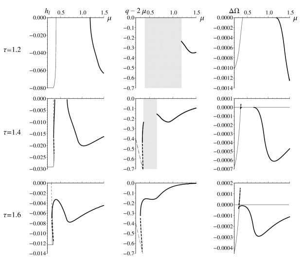
Figure 1: In each row, from left to right, we show the chemical potential dependence of the solutions for the light quarks chiral condensate, the wavelength of the modulation of the condensates (here we plot the difference $q-2\mu$ to emphasize that $q$ goes asymptotically to $2\mu$), and the thermodynamical potential difference with respect to the trivial solution for the given values of the model parameter $\tau$. Thicker lines correspond to finite-$q$ solutions. In all plots of the paper we use the units $[h]=\mathrm{GeV}^{3}$, $[\mu]=\mathrm{GeV}$, and $[\Omega]=\mathrm{GeV}^{4}$. The gray area corresponds to the interval where the value of $q$ is undetermined, as $M=0$ (see the main text for details).

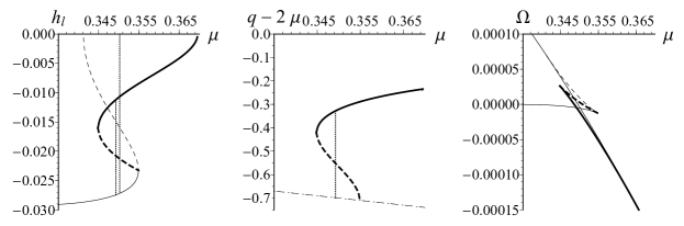
Figure 2: A zoom for chemical potential dependence of $h_{l}$, $q-2\mu$, and $\Omega$ around the first order transition point for the $\tau=1.4$ case (the same as in the second row of Fig. 1). In the leftmost panel we can see the merging of three lines, which corresponds to the annihilation of a minimum, a maximum, and a saddle point of $\Omega(h_{l},q)$. The two vertical dotted lines mark the jump (the rightmost is the usual jump when we consider only $q=0$ and the leftmost the jump to the finite $q$ solution). As before, we use thicker lines to denote the finite $q$ solutions. The diagonal straight dot-dashed line represents $q=0$.

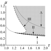
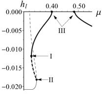
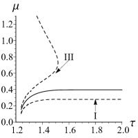
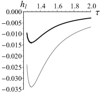
Figure 3: In 3 we present the critical chemical potentials as a function of $\tau$ in the NJL model. For $\tau<1.23$ there are two transitions: a crossover between the dynamically broken phase and the trivial phase (marked the dotted line), and, at a higher chemical potential, a transition to a phase with finite $q$ (type III, dashed line). For $\tau>1.23$ a transition to a phase with finite $q$ replaces the crossover transition. It is represented by the full line. For $1.23<\tau<1.53$ this finite-$q$ solution disappears at a critical chemical potential (marked by the lower part of the type III dashed line) but at an even higher chemical potential the preferred solution becomes again the one with finite $q$ (upper part of the type III dashed line). The shaded area marks the delimitation of the finite $q$ phase. The top-most dotted line corresponds to the choice of $\Lambda$. In 3 we plot the condensate solutions as functions of the chemical potential for the case of $\tau=1.5$ to illustrate what is meant by types I, II and III (type I finite q and h; type II vanishing q and finite h; type III vanishing h and finite q). In 3 we show the value of $q$ for the finite $q$ solutions involved in the critical points (the line types are the same as in Fig. 3). In 3 we show the condensate for the solutions with finite and vanishing $q$ (thicker for finite $q$) at the first order transition (the one which is indicated in 3 by the full line).

III.2 NJLH case

Now let us consider the extension of the model to include the strange quark and the effect of the ’t Hooft determinant. As before, we choose the model parameters in such a way as to obtain $M^{vac}_{l}=330~{}\mathrm{MeV}$. Furthermore, we chose to fix the value of $\tau$ at $1.4$. In order to better understand and differentiate the effects of flavor mixing and of the inclusion of a finite current quark mass, we consider both the case of a realistic value for the strange current mass and the chiral limit. It should be noted that in the case with the finite current mass for the strange quark the value of its dynamical mass in the vaccum depends on the coupling constant $\kappa$ ($M^{vac}_{s}=586~{}\mathrm{MeV}$ for $\kappa=0$ and $M^{vac}_{s}=542~{}\mathrm{MeV}$ for $\kappa=-2000~{}\mathrm{GeV}^{-5}$).

III.2.1 Finite strange quark current mass

Without the OZI-violating ’t Hooft determinant term ($\kappa=0$), the light and strange sectors are decoupled. The solutions obtained for $h_{l}$ are, as such, the same as in the second row of Fig. 1. An additional first order transition (at a critical chemical potential close to $M^{vac}_{s}$) appears, resulting in a jump in the value of $h_{s}$ (in this section the value considered for the current mass of the quark strange is $m_{s}=186~{}\mathrm{MeV}$).

Turning on flavor mixing couples the gap equations for the light and strange sectors. Depending on the coupling strength of the ’t Hooft determinant, we can get several different scenarios (see Fig. 4).

For $-\kappa>290~{}\mathrm{GeV}^{-5}$ a new solution branch appears with a shark-fin shape for the light condensate in the vicinity of the chemical potential corresponding to the vacuum dynamical mass of the strange quark. In the first row of Fig. 4 we present some results obtained by considering $\kappa=-500~{}\mathrm{GeV}^{-5}$, where three separate chemical potential windows with finite value of $q$ appear. With increasing chemical potential we go through two first-order transitions and three crossovers. The latter involve the dissapearance or emergence of the light condensate, as well as going to or from a finite $q$ solution to indeterminate $q$. The two first order transitions occur slightly before (for the one occuring near $M_{l}^{vac}$) and slightly above (near $M_{s}^{vac}$), thus excluding the occurrence of the $q=0$ transitions. A zoom of the behavior of the chiral condensates near the transitions can be seen in Fig. 5.

For a ’t Hooft interaction term stronger than $-\kappa>935~{}\mathrm{GeV}^{-5}$ the first two chemical potential windows with finite-$q$ solutions merge, resulting in the disappearance of the corresponding crossover transitions, as can be seen in the second row of Fig. 4.

With $-\kappa>1660~{}\mathrm{GeV}^{-5}$ the last transition to a vanishing $q$ solution does not occur and is substituted by a first-order transition between two phases with finite $q$ (see the third row of Fig. 4).

The dependence on the ’t Hooft coupling strength of the critical chemical potentials can be seen in Fig. 7.

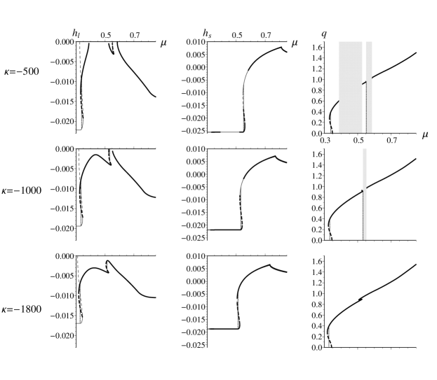
Figure 4: In each row, from left to right, we present the chemical potential dependence of the solutions for the light and strange quark chiral condensate and for the wavelength of the modulation of the condensates, for coupling strengths of the ’tHooft determinant ($\left[\kappa\right]=\mathrm{GeV}^{5}$). Thicker lines correspond to the finite-$q$ solutions. The gray area corresponds to the interval where the value of $q$ is undetermined, since $M=0$.

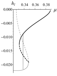
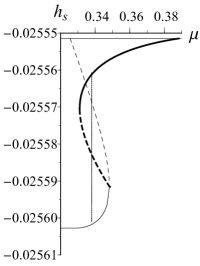
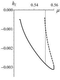
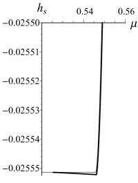
Figure 5: A zoom for the chemical dependence of the chiral condensate solutions (thicker lines refer to finite-$q$ solutions) near the transitions (marked by the vertical dotted lines), presented for the case with $\kappa=-500~{}\mathrm{GeV}^{-5}$.

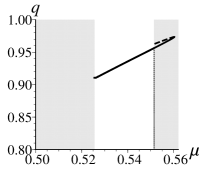
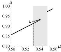
Figure 6: Zoom of the solutions for $q$ in the chemical potential window close to $M^{vac}_{s}$ for $\kappa=-500,~{}-1000,~{}-1800~{}\mathrm{GeV}^{5}$ (from left to right), showing the merging of the solution branches for strong enough flavor mixing.

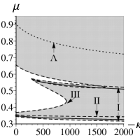
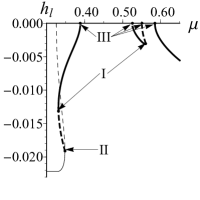
Figure 7: Critical chemical potentials as a function of the intensity of the ’t Hooft determinantal term ($[\kappa]=\mathrm{GeV}^{5}$). The upper dotted lines corresponds to the choice of the cutoff. The chemical potential of the first order transitions are marked by the full black lines. Dashed lines indicate the borders of the region where the finite-$q$ solutions exist. We distinguish between three types of critical chemical potentials and an example for this distinction in the $\kappa=-500~{}\mathrm{GeV}^{-5}$ case appears in Fig. 7 (type I with finite $q$ and $h_{l}$, type II with finite $h_{l}$ and vanishing $q$, and type III with finite $q$ but vanishing $h_{l}$).

III.2.2 ${\rm SU}_{3}$ Chiral limit

Now let us consider the effect of flavor mixing with a massless strange quark ($m_{u}=m_{d}=m_{s}=0$). For values of the ’t Hooft coupling constant lower than the critical value ($-\kappa<-\kappa_{crit}=467\mathrm{GeV}^{-5}$) this flavor mixing gives rise to the appearance of two new solution branches (these, when shifted to higher chemical potentials due to the inclusion of a finite current mass, give rise to the shark fin-like structure described in the previous section). One of these is locally stable but the global minimum still corresponds to the solution with a lower chiral condensate and a larger value of $q$ (see Fig. 8 for the $\kappa=-100~{}\mathrm{GeV}^{-5}$ example). The first order jump, which is indicated by the full line in Fig. 9, goes to a finite-$q$ solution for $-\kappa<521~{}\mathrm{GeV}^{-5}$, and to the trivial solution (vanishing chiral condensates) for stronger flavor mixing. As before, there is an additional solution branch starting at a much higher chemical potential with finite but asymptotically vanishing $h_{i}$ and $q$.

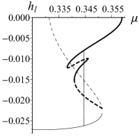
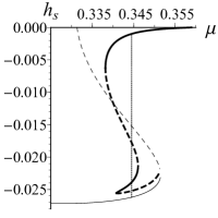
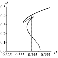
Figure 8: From left to right, we show the chemical potential dependence of the solutions for the light chiral condensate, the strange chiral condensates (thicker lines with finite $q$), and of the wavelength of the modulation $q$. The case corresponds to the chiral limit, $\tau=1.4$, and $\kappa=-100~{}\mathrm{GeV}^{-5}$. The vertical dotted line marks the first-order transition.

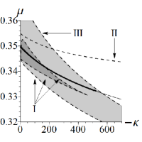
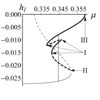
Figure 9: Critical chemical potentials for the case with flavor mixing in the chiral limit and $\tau=1.4$. Their meaning is made evident in the right-hand side panel where the light chiral condensate is shown as a function of the chemical potential for $\kappa=-100~{}\mathrm{GeV}^{-5}$ case. The shaded area indicates the existence of stable solutions with finite $q$ (light-grey: one solution, dark-grey: two solutions). A full line indicates the first order jump.

III.3 Comparison to parameter sets

In an attempt to keep the discussion in the most general terms possible, we have up to this point considered very few restrictions on the model parametrization. In Table 1 we list the values of the parameter $\tau$ extracted from several sets of parameters used in the literature (when needed, a conversion of the cutoff from the 3D case to its equivalent covariant value was done), used to fit the pseudoscalar spectrum given in Table 2 for several variants of the 3-flavor NJL model. In sets (a-c) isospin breaking was also considered, hence the values indicated in the table are the averages over the isospin multiplets. In set (c) the mixing angle is not indicated in the respective paper. Except for set (a), one observes a spread in the values of $\tau$ for the different sets comprised between $1<\tau<1.5$, and a mixing interaction strength $600<-\kappa<1800$ GeV^-5.

Despite the difference in the values for $\tau$, from the point of view of the value of $\kappa$, sets (c,e,f,g) should best fit to the case $\kappa=-1000~{}\mathrm{GeV}^{-5}$ described above, while set (b) is eventually best accomodated with $\kappa=-1800~{}\mathrm{GeV}^{-5}$, and set (d) by the $\kappa=-500~{}\mathrm{GeV}^{-5}$. From the two-flavor case one can deduce that diminishing $\tau$ corresponds to widening of the gap between the branch close to the $\mu\sim{\hat{M}}$ and the one appearing at larger values of $\mu$.

Table 1: Parameter sets of the model: $\hat{m},m_{s}$, and $\Lambda$ are given in MeV. The couplings have the following units: $[G]=$ GeV^-2, $[\kappa]=$ GeV^-5. We also show the values of constituent quark masses $\hat{M}$ and $M_{s}$ in MeV.

Sets	$\hat{m}$	$m_{s}$	$\hat{M}$	$M_{s}$	$\Lambda$	$G$	$-\kappa$	$\tau$	Ref.
a	5.5	135.7	335	527	1263	9.21	121	2.23	Hatsuda and Kunihiro (1994)
b	7.7	159	315	486	805	11.58	1775	1.14	Reinhardt and Alkofer (1988)
c	7.7	159	315	508	805	12.6	1183	1.24	Reinhardt and Alkofer (1988)
d	5.3	170	315	513	920	8.98	687	1.14	Osipov et al. (2004)
e	6.1	185	380	576	830	12.6	1116	1.32	Osipov et al. (2004)
f	5.8	183	348	544	864	10.8	921	1.23	Osipov et al. (2008)
g	6.3	194	398	588	820	13.5	1300	1.38	Osipov et al. (2006)

Table 2: The pseudoscalar masses, weak decay constans and condensates (in MeV) for the different sets. the mixing angle $\theta$ is in degrees.

Sets	$m_{\pi}$	$m_{K}$	$m_{\eta}$	$m_{\eta^{\prime}}$	$f_{\pi}$	$f_{K}$	$-<{\bar{u}}u>^{\frac{1}{3}}$	$-<{\bar{s}}s>^{\frac{1}{3}}$	$\theta$
a	138	495.7	487.	957.5	93	97.7	245	191	-21
b	140	495	502.	1244	93.3	97.7	218	178	-31
c	140	495	441.	958.	93.3	100.2	218	166
d	138	494	487.	958.	92.	121.	244	204	-12
e	138	499	477.	958.	92.	115.8	233	182	-15
f	138	494	476.	986.	92.	118.	237	191	-13.6
g	138	494	476.	986.	92.	114.	229	172	-14

IV Conclusions

We have made a thorough analysis of the instability of the strongly-interacting three-flavor quark matter at zero temperature with respect to the formation of a spatially modulated inhomogeneous phase. We have used the NJL model augmented with the ’t Hooft interations.

In the case with no flavor mixing there is a range of the model parameter $\tau$, where we obtain a finite chemical potential window with energetically favorable inhomogeneous solutions. There is a critical chemical potential above which the favored solution is always an inhomogeneous one. Above a critical value of $\tau$ these windows merge. This behavior has already been reported (albeit with a different regularization procedure) in Carignano and Buballa (2012a).

The inclusion of flavor mixing with the strange quark of a physical current mass introduces new features into the model. For a fixed value of $\tau$ and depending on the strength of the flavor mixing term we can have several scenarios. One of these is the existence of an additional finite window for an inhomogeneous phase, starting in a second order transition and ending in a first order transition (meaning there exist two first order transitions). These two chemical potential windows can also be connected, resulting in an interval (delimited by two first transitions), where the dynamical mass behaves non-monotonically. These features appear as a result of the shifting to higher chemical potential of the new solutions induced by flavor mixing due to the presence of a finite strange current mass.

There is a rich structure of solutions induced by the flavor mixing of the strange quark with the spatially modulated light-quark sector. The main highlights are:

• A new phase of globally stable inhomogeneous solutions ($q\neq 0$) emerges, covering a chemical potential interval of several tens of MeV, for chemical potential values below and in the neighborhood of the mass of the vacuum value of the strange quark mass. This phase occurs for physical strange current quark masses, as well as in the ${\rm SU}_{3}$ chiral limit, in a wide range of the values of the ’t Hooft determinant strength $\kappa$.

• Depending on the value of $\kappa$, this phase is either separated from the set of inhomogeneous solutions known to occur at chemical potentials close to the constituent quark mass of the light quarks in the vacuum, or joins with it. The interval between these two branches of solutions shrinks with the increasing value of $\kappa$ and there one only finds solutions with vanishing light quark condensates with indeterminate value of $q$.

• Besides these two branches, a third one exists at yet higher chemical potential (larger than the strange quark mass). This type of solutions were discussed in the literature in connection with the the ${\rm SU}_{2}$ case, and are present in our three-flavor study as well.

• Above a certain critical value of $\kappa$, there is a first order transition which connects the solutions with different values of $q$, which prevail as being the globally stable ones in the asymptotic regime $q\rightarrow 2\mu$.

• In the chiral limit, these branches of inhomogeneous solutions have overlapping chemical potential windows. Interestingly, one of the branches has in this case a strange condensate which is lower (in absolute value) than the light condensate and is the globally stable solution.

We conclude that flavor mixing acts as a catalyst for the emergence of globally stable inhomogeneous solutions in zero-temperature quark matter.