Interval-Valued Rank in Finite Ordered Sets

Abstract

We consider the concept of rank as a measure of the vertical levels and positions of elements of partially ordered sets (posets). We are motivated by the need for algorithmic measures on large, real-world hierarchically-structured data objects like the semantic hierarchies of ontological databases. These rarely satisfy the strong property of gradedness, which is required for traditional rank functions to exist. Representing such semantic hierarchies as finite, bounded posets, we recognize the duality of ordered structures to motivate rank functions which respect verticality both from the bottom and from the top. Our rank functions are thus interval-valued, and always exist, even for non-graded posets, providing order homomorphisms to an interval order on the interval-valued ranks. The concept of rank width arises naturally, allowing us to identify the poset region with point-valued width as its longest graded portion (which we call the “spindle”). A standard interval rank function is naturally motivated both in terms of its extremality and on pragmatic grounds. Its properties are examined, including the relationship to traditional grading and rank functions, and methods to assess comparisons of standard interval-valued ranks.

1 Introduction

A characteristic of partial orders and partially ordered sets (posets) as used in order theory [9] is that they are amongst the simplest structures which can be called “hierarchical” in the sense of admitting to descriptions in terms of levels. And yet we have found that the mathematical development of the concepts of level, “depth”, or “rank” is surprisingly incomplete. Rank is used in order theory in two related senses:

• First, the rank function (if it exists) of a poset is a canonical scalar monotonic function representing the vertical level of each element. However, this concept has been literally one-sided, requiring a bias towards a particular “pointing” of the poset as being either “top down” or “bottom up”, arbitrarily.

• And secondly, a poset as a whole can be graded, or “have rank”, meaning that there exists such a rank function which assigns each element a unique vertical level consistent with its covering structure, such that a single step in the hierarchy results in a single increment or decrement of rank. But while graded posets dominate the primary results in formal lattice theory [6], this is a strong property. Real-world data objects with hierarchical structure cannot generally be assumed to be graded, and in certain fields virtually none of them are.

We thus seek a concept of rank in general finite posets, whether graded or not. We believe that this goal is satisfied naturally by extending rank to be intervally-valued, and to use interval orders to compare the vertical level of components of hierarchies.

Our motivation is from the kinds of hierarchically-structured data objects which abound in computer science, and especially the semantic typing systems of modern knowledge systems such as ontological databases and object-oriented typing hierarchies. These structures are built around semantic hierarchies as their cores. These, in turn, are collections of objects (classes or linguistic concepts) which are organized into hierarchies such as taxonomic (subsumptive, “is-a”); meronomic (compositional, “has-part”); and implication (logical, “follows-from”) relations. Prominent examples include WordNet in the computational linguistics community [11] and the Gene Ontology (GO) in the computational genomics community [3]. Fig. 1 shows a portion of the GO. Black text indicates nodes representing biological processes, and are arranged in a directed acyclic graph (DAG) representing subsumption (e.g. “DNA repair” is a kind of “DNA metabolism”). The names of genes from three species of model organism are shown in colored text as “annotations” to these nodes, indicating that those genes perform those functions.

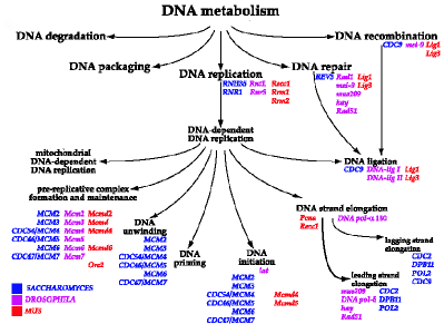
Figure 1: A portion of the Biological Process branch of the Gene Ontology (adapted from [3]). The database is structured as a large, top-rooted directed acyclic graph of genomic functional categories, labeled with the genes of multiple species.

Fig. 1 shows only a small fragment of one portion of the GO. But typical of many such real-world semantic hierarchies, the GO has grown to be quite large, currently over thirty thousand concepts. As the number and size of semantic hierarchies grows, it is becoming critical to have computer systems which are appropriate for managing them, and especially important to complement manual methods with algorithmic approaches to tasks such as construction, alignment, annotation, and visualization. These tasks in turn require us to have a solid mathematical grounding for the analysis of semantic hierarchies, and especially the ability to measure entire hierarchies and portions of hierarchies using such concepts as distances and sizes of regions.

One particular aspect of hierarchical structure which needs to be measurable is the placement of elements vertically relative to each other in ranks or levels. This is critical, for example, in visualization applications. Fig. 2 (from [18]), shows a visualization of a GO portion, wherein the vertical layout over a large hierarchical structure is essential.

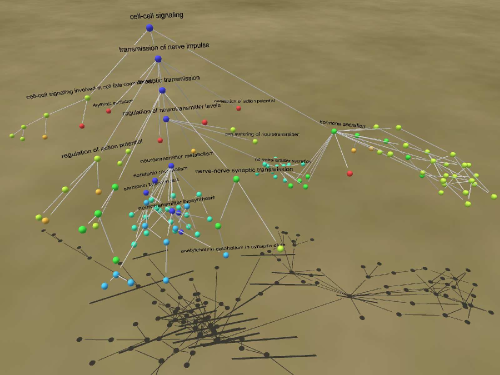
Figure 2: An example ontology layout result, from [18].

As mathematical data objects, semantic hierarchies resemble top-rooted trees. But with the presence of significant amounts of “multiple inheritance” (nodes having more than one parent, as for “DNA ligation” in Fig. 1), and also the possible inclusion of transitive links, they must in general be represented at most as DAGs. And since the primary semantic categories of subsumption and composition are transitive, the proper mathematical grounding for such algorithms and measures is order theory, representing semantic hierarchies as posets.

While order theory offers a fundamental formalization of hierarchy in general, it has been largely neglected in knowledge systems technology, and we believe it has promise in the development of tools for managing semantic hierarchies. The most prominent approaches to managing the GO and WordNet are effectively ad hoc and de novo (e.g. [7]). And conversely, even outside of the domain of knowledge systems applications, the precise formulation in ordered sets of concepts such as distance and dispersion are little known and in many cases underdeveloped in the first place. Our prior work [15, 16, 19, 20, 28] has advanced the use of measures of distance and similarity, and characterizations of mappings and linkages within semantic hierarchies.

Semantic hierarchies are rarely graded, so the standard concepts of rank and grade are not especially useful for dealing with measuring and laying out their vertical levels. In this paper, we seek a coherent formulation of vertical element placement in posets. We begin with some notational elements about posets, maximal chains, maximum chains (which we call the spindle), and order morphisms. We then introduce concepts and notation for integer intervals and operations thereon, including our treatment of interval orders, including strong, weak, and subset orders. We use these tools to consider the general sense of rank and vertical rank in posets as a necessarily two-sided concept, motivating rank as an interval-valued function inducing a strict order morphism to some interval order. Cases are considered, and then a strict version of an interval rank function is introduced, which preserves strict homomorphism not just for the intervals overall, but also for their constituent endpoints as well.

We can identify a particular interval rank function for the weak interval order, which we call the standard interval rank function. We point out that this standard interval rank function is special both on the basis of its extremality, and as derived from a procedural approach to natural scalar-valued rank. We consider some properties of the standard interval rank, and the use of interval analysis to be able to compare interval-valued ranks in terms of their interval-valued separation. In this way, we can gain a sense of the vertical distances between even non-comparable poset elements.

2 Preliminaries

Throughout this paper we will use $\mathbb{N}$ to denote $\{0,1,\ldots\}$, the set of integers greater than or equal to 0, and for $N\in\mathbb{N}$, the set of integers between 0 and $N$ will be denoted $\mathbb{N}_{N}\mathrel{\bf\colon\kern-2.0pt=}\{0,1,\ldots,N\}$.

2.1 Ordered Sets

See e.g. [9, 24, 26] for the basics of order theory, the following is primarily for notational purposes.

Let $P$ be a finite set of elements with $|P|\geq 2$, and $\leq$ be a binary relation on $P$ (a subset of $P^{2}$) which is reflexive, transitive, and antisymmetric. Then $\leq$ is a partial order, and the structure ${\cal P}=\left<P,\leq\right>$ is a partially ordered set (poset). $a<b$ means that $a\leq b$ and $a\neq b$, and is a strict order on $P$, which is an irreflexive partial order. A strict order $<$ can be turned into a partial order through reflexive closure: $\leq\mathrel{\bf\colon\kern-2.0pt=}<\cup\,\{\left<a,a\right>\in P^{2}\}$.

For any pair of elements $a,b\in P$, we say $a\leq b\in P$ to mean that $a,b\in P$ and $a\leq b$. And for $a\in P,Q\subseteq P$, we say $a\leq Q$ to mean that $\forall b\in Q,a\leq b$. If $a\leq b\in P$ or $b\leq a\in P$ then we say that $a$ and $b$ are comparable, denoted $a\sim b$. If not, then they are incomparable, denoted $a\|b$. For $a,b\in P$, let $a\prec b$ be the covering relation where $a\leq b$ and $\nexists c\in P$ with $a<c<b$.

A set of elements $C\subseteq P$ is a chain if $\forall a,b\in C,a\sim b$. If $P$ is a chain, then ${\cal P}$ is called a total order. A chain $C\subseteq P$ is maximal if there is no other chain $C^{\prime}\subseteq P$ with $C\subseteq C^{\prime}$. Naturally all maximal chains are saturated, meaning that $C=\{a_{i}\}_{i=1}^{|C|}\subseteq P$ can be sorted by $\leq$ and written as $C=a_{1}\prec a_{2}\prec\ldots\prec a_{|C|}$. The height $0pt({\cal P})$ of a poset is the size of its largest chain. Below we will use $0pt$ alone for $0pt({\cal P})$ when clear from context.

For any subset of elements $Q\subseteq P$, let $\left.{\cal P}\right|_{Q}=\left<Q,\leq_{Q}\right>$ be the sub-poset determined by $Q$, so that for $a,b\in Q$, $a\leq_{Q}b\in Q$ if $a\leq b\in P$.

For any element $a\in P$, define the up-set or principal filter $\mathop{\uparrow}a\mathrel{\bf\colon\kern-2.0pt=}\{b\in P\mathrel{\colon}b\geq a\}$, down-set or principal ideal $\mathop{\downarrow}a\mathrel{\bf\colon\kern-2.0pt=}\{b\in P\mathrel{\colon}b\leq a\}$, and hourglass $\Xi(a)\mathrel{\bf\colon\kern-2.0pt=}\mathop{\uparrow}a\cup\mathop{\downarrow}a$. For $a\leq b\in P$, define the interval $[a,b]\mathrel{\bf\colon\kern-2.0pt=}\{c\in P\mathrel{\colon}a\leq c\leq b\}=\mathop{\uparrow}a\cap\mathop{\downarrow}b$.

For any subset of elements $Q\subseteq P$, define its maximal and minimal elements as

$${\rm Max}(Q)\mathrel{\bf\colon\kern-2.0pt=}\{a\in Q\mathrel{\colon}{\nexists}b\in Q,a<b\}\subseteq Q$$

$${\rm Min}(Q)\mathrel{\bf\colon\kern-2.0pt=}\{a\in Q\mathrel{\colon}{\nexists}b\in Q,b<a\}\subseteq Q,$$

called the roots and leaves respectively. Except where noted, in this paper we will assume that our posets ${\cal P}$ are bounded, so that $\bot\leq\top\in P$ with ${\rm Max}(P)=\{\top\},{\rm Min}(P)=\{\bot\}$. Since we’ve disallowed the degenerate case of $|P|=1$, we have $\bot<\top\in P$. All intervals $[a,b]$ are bounded sub-posets, and since ${\cal P}$ is bounded, $\forall a\in P,\mathop{\uparrow}a=[a,\top],\mathop{\downarrow}a=[\bot,a]$, and thus $\bot,\top\in\Xi(a)\subseteq{\cal P}=[\bot,\top]$. An example of a bounded poset and a sub-poset expressed as an hourglass is shown in Fig. 3.

Figure 3: (Left) The Hasse diagram (canonical visual representation of the covering relation $\prec$) of an example bounded poset ${\cal P}$. (Right) The Hasse diagram of the sub-poset $\left.{\cal P}\right|_{\Xi(J)}$ for the hourglass $\Xi(J)=\mathop{\uparrow}J\cup\mathop{\downarrow}J=[J,\top]\cup[\bot,J]=\{J,C,K,\top\}\cup\{\bot,J\}=\{\bot,C,J,K,\top\}$.

The following properties are prominent in lattice theory, and are available for some of the highly regular lattices and posets that appear there (see e.g. Aigner [1]).

Definition 1: (Jordan-Dedekind Condition)

A poset ${\cal P}$ has the Jordan-Dedekind condition (we say that ${\cal P}$ is JD) when all saturated chains (note: not just maximal chains) connecting two elements $a\leq b\in P$ are the same size.

Definition 2: (Rank Function and Graded Posets)

For a top-bounded poset ${\cal P}$, a function $\rho\colon P\rightarrow\mathbb{N}_{0pt-1}$ is a rank function when $\rho(\top)=0$ and $\forall a\prec b\in P,\rho(a)=\rho(b)-1$. A poset ${\cal P}$ is graded, or fully graded, if it has a rank function.

Theorem 3.

[6] A poset ${\cal P}$ is graded iff it is JD.

Let ${\cal C}({\cal P})\subseteq 2^{P}$ be the set of all maximal chains of ${\cal P}$. We assume that ${\cal P}$ is bounded, therefore $\forall C\in{\cal C}({\cal P}),\bot,\top\in C$. For any element $a\in P$, define its centrality as the length of the largest maximal chain it sits on, i.e., the height of its hourglass

$$S(a)\mathrel{\bf\colon\kern-2.0pt=}0pt(\Xi(a))=0pt(\mathop{\uparrow}a)+0pt(\mathop{\downarrow}a)-1.$$

We will refer to the spindle chains of a poset ${\cal P}$ as the set of its maximum length chains

$${\cal I}({\cal P})\mathrel{\bf\colon\kern-2.0pt=}\left\{C\in{\cal C}({\cal P})\mathrel{\colon}|C|=0pt\right\}.$$

The spindle set

$$I({\cal P})\mathrel{\bf\colon\kern-2.0pt=}\bigcup_{C\in{\cal I}({\cal P})}C\subseteq P$$

is then the set of spindle elements, including any elements which sit on a spindle chain. Note that if $P$ is nonempty (as we require) then there is always at least one spindle chain and thus at least one spindle element, so also ${\cal I}({\cal P}),I({\cal P})\neq\emptyset$.

In our example in Fig. 3, we have $0pt=5$, $|{\cal C}({\cal P})|=6$, ${\cal I}({\cal P})=\{\bot\prec A\prec H\prec K\prec\top\}$, and $S(J)=0pt(\mathop{\uparrow}J)+0pt(\mathop{\downarrow}J)-1=4$.

Given two posets ${\cal P}_{1}=\left<P,\leq_{P}\right>$ and ${\cal P}_{2}=\left<Q,\leq_{Q}\right>$, a function $f\colon P\rightarrow Q$ is an order homomorphism provided $a\leq_{P}b\in P\implies f(a)\leq_{Q}f(b)$. Compare to the stronger, and possibly more familiar notion of an order embedding [9] where $a\leq_{P}b\iff f(a)\leq_{Q}f(b)$. In this paper we will only be using order homomorphisms which simply map the structure of one partial order into another without the reverse needing to be true. We can also say that $f$ preserves the order $\leq_{P}$ into $\leq_{Q}$, and is an isotone mapping from ${\cal P}_{1}$ to ${\cal P}_{2}$. If $\forall a<_{P}b\in P,f(a)<_{Q}f(b)\in Q$ then we say that $f$ does all this strictly. If instead $f$ is an order homomorphism from ${\cal P}_{1}$ to the dual $\left<Q,\geq_{Q}\right>$, then we say that $f$ reverses the order, or $f$ is an antitone mapping. If $f\colon P\rightarrow Q$ is an order homomorphism, then we can denote $f({\cal P}_{1})\mathrel{\bf\colon\kern-2.0pt=}\left<f(P),\leq_{f}\right>$ as the homomorphic image of ${\cal P}_{1}$, with

$$f(P)\mathrel{\bf\colon\kern-2.0pt=}\{f(a)\mathrel{\colon}a\in P\}\subseteq Q,\quad\leq_{f}\,\,\mathrel{\bf\colon\kern-2.0pt=}\leq_{Q}\!\left|{}_{f(P)\times f(P)}\right.$$

When clear from context, we will simply re-use $\leq$ as the relevant order to its base set, e.g. for an isotone $f\colon P\rightarrow Q,a\leq b\in P\implies f(a)\leq f(b)\in Q$.

Finally, we recognize $\left<\mathbb{N},\leq\right>$ as a total order using the normal numeric order $\leq$, and observe that for any bounded poset ${\cal P}$, the functions $0pt(\mathop{\uparrow}\cdot),0pt(\mathop{\downarrow}\cdot):P\rightarrow\mathbb{N}_{0pt}$ induce strict antitone and isotone order morphisms, respectively. That is, if $a\prec b$ then

$$0pt(\mathop{\uparrow}a)\geq 0pt(\mathop{\uparrow}b)+1>0pt(\mathop{\uparrow}b)\qquad\text{and}\qquad 0pt(\mathop{\downarrow}a)<0pt(\mathop{\downarrow}a)+1\leq 0pt(\mathop{\downarrow}b).$$

2.2 Numeric Intervals: Operations and Orders

Since our rank functions will be interval-valued, we explicate the concepts surrounding the possible ordering relations among intervals. Our formulation is a bit nonstandard, but helpful for this particular application. Our view actually resonates with algebraic approaches to interval analysis used in artificial intelligence, such as Allen’s interval algebra [2, 21, 22]. But these methods are not order-theoretical, nor are we aware of prior use of our weak interval order $\leq_{W}$ in interval analysis proper. We begin by defining operations on intervals before going into orders among intervals.

$\left<\mathbb{R},\leq\right>$ is a total order, so for any $x_{*}\leq x^{*}\in\mathbb{R}$, we can denote the (real) interval $\bar{x}=[x_{*},x^{*}]$, and $\overline{\mathbb{R}}$ as the set of all real intervals on $\mathbb{R}$, so that $\bar{x}\in\overline{\mathbb{R}}$. Additionally, for $N\in\mathbb{N}$ let $\overline{N}$ be the set of all intervals whose endpoints are nonnegative integers $\leq N$. We define the interval midpoint $\hat{\bar{x}}=\frac{x_{*}+x^{*}}{2}\in\mathbb{R}$ and interval width $W(\bar{x})\mathrel{\bf\colon\kern-2.0pt=}|x^{*}-x_{*}|\in\mathbb{R}$.

Operations on real intervals (see e.g. [23]) are defined setwise, so that for $\bar{x},\bar{y}\in\overline{\mathbb{R}}$ and a unary or binary operation $\bullet$,

$$\bullet(\bar{x})\mathrel{\bf\colon\kern-2.0pt=}\{\bullet(z):z\in\bar{x}\},\qquad\bar{x}\bullet\bar{y}\mathrel{\bf\colon\kern-2.0pt=}\{z_{1}\bullet z_{2}:z_{1}\in\bar{x},z_{2}\in\bar{y}\}.$$

This yields specific real interval operations of addition $\bar{x}+\bar{y}\mathrel{\bf\colon\kern-2.0pt=}[x_{*}+y_{*},x^{*}+y^{*}]$ (often referred to as the Minkowski sum [5]); subtraction $\bar{x}-\bar{y}\mathrel{\bf\colon\kern-2.0pt=}[x_{*}-y^{*},x^{*}-y_{*}]$; and absolute value $|\bar{x}|=[|\bar{x}|_{*},|\bar{x}|^{*}]$, where

$$|\bar{x}|_{*} \mathrel{\bf\colon\kern-2.0pt=}\left\{\begin{array}[]{ll}0&x_{*}x^{*}\leq 0\\ \min(|x_{*}|,|x^{*}|)&x_{*}x^{*}>0\end{array}\right.$$

$$|\bar{x}|^{*} \mathrel{\bf\colon\kern-2.0pt=}\max(|x_{*}|,|x^{*}|).$$

We also have the separation $\|\bar{x},\bar{y}\|\mathrel{\bf\colon\kern-2.0pt=}|\bar{x}-\bar{y}|$, an interval valued function of two intervals which represents the interval between the minimum and maximum difference between any two chosen points, one from each interval.

In the literature [4, 12, 13, 27] the standard ordering on a set of intervals $P$ is a binary relation $\leq$ satisfying the Ferrers property [8, 10], so that $\forall x,y,z,w\in P,x\leq y,z\leq w$ implies $x\leq w$ or $z\leq y$. This results in the almost completely universal recognition of the term “interval order” to mean what we call here the strong interval order $\leq_{S}$. While it is the only interval order we consider here which satisfies Ferrers, it is only one possible order on real intervals. It is the strongest, but also the least useful for our purposes compared to the others, although they are much less widely recognized.

Definition 4: (Strong Interval Order)

Let $<_{S}$ be a strict order on $\overline{\mathbb{R}}$ where $\bar{x}<_{S}\bar{y}$ iff $x^{*}<y_{*}$. Let $\leq_{S}$ be the reflexive closure of $<_{S}$, so that $\bar{x}\leq_{S}\bar{y}$ iff $x^{*}<y_{*}$ or $\bar{x}=\bar{y}$.

In addition to the strong interval order $\leq_{S}$, some [25] recognize $\subseteq$ as an interval-containment or subset interval order.

Definition 5: (Subset Interval Order)

Let $\subseteq$ be a partial order on $\overline{\mathbb{R}}$ where $\bar{x}\subseteq\bar{y}$ iff $x_{*}\geq y_{*}$ and $x^{*}\leq y^{*}$.

But one of the most natural ordering relations between two intervals is given by the product order $\leq\times\leq$ based on $\left<\mathbb{R},\leq\right>$. We call this the weak interval order (not to be confused with Fishburn’s weak order [13], which is different).

Definition 6: (Weak Interval Order)

Let $\leq_{W}$ be a partial order on $\overline{\mathbb{R}}$ where $\bar{x}\leq_{W}\bar{y}$ iff $x_{*}\leq y_{*}$ and $x^{*}\leq y^{*}$.

These three orders on $\overline{R}$ are related as follows.

• As their names suggest, the strong order implies the weak order: if $\bar{x}\leq_{S}\bar{y}$ then $\bar{x}\leq_{W}\bar{y}$.

• The weak order and subset order are related. Notice that if two intervals are properly weakly ordered (i.e., $\bar{x}<_{W}\bar{y}$ and none of the endpoints are equal) then the intervals are not comparable in the subset order. Dually, if two intervals are properly subset ordered ($\bar{x}\subset\bar{y}$ and none of the endpoints are equal) then the intervals are not comparable in the weak order. This notion of being comparable in one or the other, but not both, is called conjugacy. It is an interesting topic, but one we leave for consideration in future work [17].

Based on these observations, we can identify two additional orders available on real intervals:

• The dual to $\leq_{W}$ is $\bar{x}\geq_{W}\bar{y}$, so that $\geq_{W}=\geq\times\geq$.

• The dual to the subset order is the superset order, so that $\supseteq=\leq\times\geq$.

Here we introduce the notation $\bar{x}\circ_{\leq}\bar{y}$ to mean “properly intersecting from the left”, meaning

$$\bar{x}\circ_{\leq}\bar{y}\mathrel{\bf\colon\kern-2.0pt=}\bar{x}\leq_{W}\bar{y},\bar{x}\not\leq_{S}\bar{y}.$$

There is also the dual “properly intersecting from the right”:

$$\bar{x}\circ_{\geq}\bar{y}\mathrel{\bf\colon\kern-2.0pt=}\bar{x}\geq_{W}\bar{y},\bar{x}\not\geq_{S}\bar{y}.$$

We will refer back to this in Section 4.2. Note that $\circ_{\leq}$ and $\circ_{\geq}$ are not themselves partial orders, since they are not transitive. But when we assume for simplicity that no two of $x_{*},x^{*},y_{*}$, and $y^{*}$ are equal (per discussion above), then any pair of intervals $\bar{x},\bar{y}$ will stand in exactly one of these three binary relations $\bar{x}\bowtie\bar{y}$ for $\bowtie\in\{<_{S},\circ_{\leq},\subset\}$, or their duals.

Later we will be interested in comparing intervals standing in different order relations $\bowtie$; that is, calculating differences $\bar{y}-\bar{x}$ and separations $\|\bar{x},\bar{y}\|$. Let $\bar{\alpha}=\bar{y}-\bar{x}=[y_{*}-x^{*},y^{*}-x_{*}]$, and consider the three situations shown in Fig. 4, again assuming that no two of $x_{*},x^{*},y_{*}$, or $y^{*}$ are equal. Then for the three cases $\bowtie\in\{<_{S},\circ_{\leq},\subset\}$, the quantitative relations among the components of $\bar{x},\bar{y},\bar{a}=\bar{y}-\bar{x},\|\bar{x},\bar{y}\|$, and the width $W(\|\bar{x},\bar{y}\|)$ are shown in Table 1. Similar results hold for the dual cases $\bowtie\in\{>_{S},\circ_{\geq},\supset\}$.

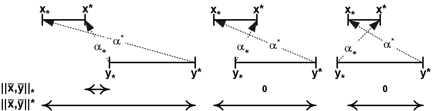
Figure 4: The three qualitative interval relations, including the separation interval $\|\bar{x},\bar{y}\|=[\|\bar{x},\bar{y}\|_{*},\|\bar{x},\bar{y}\|^{*}]$. (Left) $\bar{x}<_{S}\bar{y}$. (Center) $\bar{x}\circ_{\leq}\bar{y}$. (Right) $\bar{x}\subset\bar{y}$.

$\bar{x}\bowtie\bar{y}$		$\bar{\alpha}=\bar{y}-\bar{x}=[y_{*}-x^{*},y^{*}-x_{*}]$		$\|\bar{x},\bar{y}\|$	$W(\|\bar{x},\bar{y}\|)$
$\bar{x}<_{S}\bar{y}$	$x_{*}<x^{*}<y_{*}<y^{*}$	$[0,0]<_{S}\bar{\alpha}$	$0<\alpha_{*}<\alpha^{*}$	$\bar{\alpha}=[\alpha_{*},\alpha^{*}]$	$\alpha^{*}-\alpha_{*}$
$\bar{x}\circ_{\leq}\bar{y}$	$x_{*}<y_{*}<x^{*}<y^{*}$	$[0,0]\subset\bar{\alpha}$	$\alpha_{*}<0<-\alpha_{*}<\alpha^{*}$	$[0,\alpha^{*}]$	$\alpha^{*}$
$\bar{x}\subset\bar{y}$	$y_{*}<x_{*}<x^{*}<y^{*}$	$[0,0]\subset\bar{\alpha}$	$\alpha_{*}<0<\alpha^{*}$	$[0,{\rm Max}(-\alpha_{*},\alpha^{*})]$	${\rm Max}(-\alpha_{*},\alpha^{*})$

Table 1: Relations among quantities of interval difference depending on order relation, assume in all cases that no two of $x_{*},x^{*},y_{*}$, and $y^{*}$ are equal.

In closing this section, we note that while these ordering relations $\leq_{S},\subseteq$, and $\leq_{W}$ are defined here for real intervals in the chain $\left<\mathbb{R},\leq\right>$, in fact they are also available for general intervals in arbitrary posets $\left<P,\leq\right>$, something which we have started to explore elsewhere [30].

3 Interval Rank

Consider again the fragment of the GO in Fig. 1. This is typical of our problem domain, where data structures are top-bounded DAGs, with a moderate amount of multiple inheritance (multiple parents per node), branching downward very strongly (on average many children per node, and many more than parents), and whose transitive closures are not required to be join semi-lattices, but typically are (in other words, it may be the case that $\exists a,b\in P,|{\rm Min}(\mathop{\uparrow}a\cap\mathop{\uparrow}b)|>1$). We model these structures as finite bounded posets ${\cal P}$ by taking their transitive closures and augmenting $P$ to include a bottom bound $\bot\in P$ such that $\forall a\in P,\bot\leq a$. We also include a top bound if one doesn’t already exist.

For pragmatic purposes related to historical usage in the computer science community, we want ${\cal P}$ to be “pointed” so that the top bound $\top\in P$ is up, but with rank 0, with ranks growing as we descend and shrinking as we ascend. This introduces regrettable terminological and notational complexity, and in particular the need to work in origin zero, which makes counting difficult; and primarily with antitone (order reversing), rather than isotone (order preserving), functions, as will be seen below.

Our development then begins in earnest by considering the typical approach used in applications: count the vertical level of a node as how “far” it is down from the top $\top\in P$, usually in terms of some kind of path length, and perhaps relative to the total height $0pt$. In Fig. 1, $\top=$ “DNA metabolism”, and $0pt=5$ (here considering $\mathcal{P}$ unbounded). However, compare the node “DNA degradation” with the node “lagging strand elongation”. Despite being in quite different apparent vertical locations relative to $\top$ (one and four down from $\top$ respectively), they share something in common, namely that they are both leaves. Thus in fact they (and all the leaves) are at the bottom, no matter how far they may also be from the top. So once the bottom $\bot$ is inserted, these leaves $L={\rm Min}(P)$ of our original DAG are, in fact, all also “one up” from it: $\bot\prec L$.

So it is imperative to consider the level of an element $a\in P$ not as a one-sided distance from a privileged direction in which the poset has been pointed, but as a joint concept, involving the distance of $a$ from the top $\top$, yes, but also from the bottom $\bot$, all in the context of the total height of the poset. And furthermore, these distances are separate, since as we have seen, elements can be either close to or far from either the top or bottom independently. This motivates considering overall rank as being better represented by these two independent numerical “levels”, and thus as a real interval between them.

3.1 Interval Rank Functions

We use these principles to characterize, with as few preconsiderations as possible, the vertical structure of a poset in terms of a rank function value $R(a)$ for each poset element $a\in P$. We favor rank functions satisfying:

• Rank $R$ should be an interval-valued function on $P$.

• Endpoints of these interval-valued ranks should be integers between 0 and $0pt-1$ (to accommodate our origin zero counting).

• Ranks should be monotone, and in particular preferably antitone (increasing as we descend from $\top\in P$, and decreasing as we ascend from $\bot\in P$) rather than isotone (the reverse).

We begin formalizing this as follows.

Definition 7: (Interval Rank Function)

Let ${\cal P}=\left<P,\leq\right>$ be a poset and $\sqsubseteq$ an order on real intervals. Then a function, $R_{\sqsubseteq}\colon P\rightarrow\overline{\mathbb{N}}$, with $R_{\sqsubseteq}(a)=[r_{*}(a),r^{*}(a)]$ for $a\in P$, is an interval rank function for $\sqsubseteq$ if $R_{\sqsubseteq}$ is a strict order homomorphism $\mathcal{P}\mapsto\left<\overline{\mathbb{N}},\sqsubseteq\right>$, i.e., for all $a<b$ in $\mathcal{P}$ we have $R_{\sqsubseteq}(a)\sqsubset R_{\sqsubseteq}(b)$. Let ${\bf R}_{\sqsubseteq}({\cal P})$ be the set of all interval rank functions $R_{\sqsubseteq}$ for the interval order $\sqsubseteq$ on a poset ${\cal P}$.

Below we will frequently omit the subscript and simply use $R$ when clear from context. Note the value provided by a strict order homomorphism in Def. 7, since without strictness any function $R(a)$ which $\forall a\in P,R(a)=[r,r]$ for some constant $r\in\mathbb{N}$ would be a valid interval rank function for any interval order.

When $r_{*}(a)=r^{*}(a)$, then denote $r(a)\mathrel{\bf\colon\kern-2.0pt=}r_{*}(a)=r^{*}(a)$. Let $W_{R}(a)\mathrel{\bf\colon\kern-2.0pt=}W(R(a))\in\mathbb{N}_{N}$ be the rank width for interval rank function $R$ (or just $W(a)$ when clear from context), and

$$\widehat{R(a)}\mathrel{\bf\colon\kern-2.0pt=}\frac{r_{*}(a)+r^{*}(a)}{2}\in\mathbb{R}$$

be the rank midpoint. We will say that an element $a\in P$ is precisely ranked if $W(a)=0$, and a set of elements $Q\subseteq P$ is precisely ranked if all $a\in Q$ are precisely ranked.

Where Def. 7 captures monotonicity of the interval ranks, does it follow that their constituent endpoints are also monotonic? The answer is yes for the interval orders defined in Section 2.2.

Proposition 8.

Let $R_{\sqsubseteq}(a)=[r_{*}(a),r^{*}(a)]:\mathcal{P}\rightarrow\overline{\mathbb{N}}$ be an interval rank function for interval order $\sqsubseteq$. Then, $r_{*}(a)$ and $r^{*}(a)$ are monotonic functions iff $\sqsubseteq\in\{\leq_{W},\geq_{W},\subseteq,\supseteq\}$. In particular:

1. $r_{*}$ and $r^{*}$ are isotone iff $\sqsubseteq=\leq_{W}$ .

2. $r_{*}$ and $r^{*}$ are antitone iff $\sqsubseteq=\geq_{W}$.

3. $r_{*}$ is antitone and $r^{*}$ is isotone iff $\sqsubseteq=\subseteq$.

4. $r_{*}$ is isotone and $r^{*}$ is antitone iff $\sqsubseteq=\supseteq$.

Proof.

$(\Longleftarrow)$

Here we assume that $\sqsubseteq\in\{\leq_{W},\geq_{W},\subseteq,\supseteq\}$ and need to show that $r_{*}$ and $r^{*}$ are monotonic functions of the forms above. We will just prove (i) here and observe that the rest of the cases follow analogously. Let $R_{\leq_{W}}(a)=[r_{*}(a),r^{*}(a)]$ be an interval rank function for the weak interval order. Then, if $a<b\in P$ we know from Def. 7 that $R_{\leq_{W}}(a)<_{W}R_{\leq_{W}}(b)$. But this simply means that

$$r_{*}(a)\leq r_{*}(b)\text{ and }r^{*}(a)\leq r^{*}(b),$$

and therefore both $r_{*}$ and $r^{*}$ are isotone. Similarly for the other three cases we see that requiring a strict order homomorphism implies monotonicity conditions on the endpoints of the intervals.

$(\Longrightarrow)$

Now we assume that $r_{*}$ and $r^{*}$ are monotonic functions, and that $R_{\sqsubseteq}=[r_{*},r^{*}]$ is an interval rank function. We must show that each of the four ways in which $r_{*}$ and $r^{*}$ are both monotonic we have a unique interval order. This time, let us assume that $r_{*}$ is antitone and $r^{*}$ is isotone (so we are in case (iii)). If $a<b\in\mathcal{P}$ we know that

$$r_{*}(a)\geq r_{*}(b)\quad\text{ and }\quad r^{*}(a)\leq r^{*}(b).$$

This is exactly $R_{\sqsubseteq}(a)\subseteq R_{\sqsubseteq}(b)$. But of course we assumed $R_{\sqsubseteq}$ was an interval rank function, so $R_{\sqsubseteq}(a)\subset R_{\sqsubseteq}(b)$. Since $a$ and $b$ were chosen arbitrarily we know that $R_{\sqsubseteq}$ must be a strict order homomorphism into $\overline{\mathbb{N}}$ with the $\subseteq$ ordering. So $\sqsubseteq=\subseteq$ as desired. The other three cases follow similarly.

∎

Proposition 8 applies to the four interval orders, $\leq_{W},\geq_{W},\subseteq,\supseteq$, as there are only four ways for both endpoints to be monotone, and each corresponds to one of these four interval orders. The rank function for the strong interval order $\leq_{S}$ is derived easily as a case of the weak order $\leq_{W}$.

Corollary 9.

Let $R_{\sqsubseteq}(a)=[r_{*}(a),r^{*}(a)]:\mathcal{P}\rightarrow\overline{\mathbb{N}}$ be an interval rank function for interval order $\leq_{S}$ (resp. $\geq_{S}$). Then, $r_{*}(a)$ and $r^{*}(a)$ are both isotone (resp. antitone).

Proof.

We have previously observed that if $\overline{x}\leq_{S}\overline{y}$ then $\overline{x}\leq_{W}\overline{y}$, i.e., the strong interval order implies the weak interval order. Therefore if $R_{\sqsubseteq}$ is an interval rank function for $\leq_{S}$ then it is also an interval rank function for $\leq_{W}$. So by Proposition 8(i) we know that $r_{*}(a)$ and $r^{*}(a)$ are both isotone. And if $\sqsubseteq=\geq_{S}$ then $r_{*}(a)$ and $r^{*}(a)$ are both antitone (Prop 8(ii)). ∎

Since $\leq_{S}$ implies $\leq_{W}$, but not vice versa, Corollary 9 is not a bi-implication, like Proposition 8. Fig. 5 shows a partial order adorned with an interval-valued function with both endpoints antitone on each of its elements which holds for $\leq_{W}$, but not $\leq_{S}$.

Figure 5: A poset with interval valued strict antitone function which is an interval rank function for the weak order, but not for the strong order.

We noted that strict interval orders play a critical role in Def. 7 to avoid degeneracies like $R(a)=[r,r]$. But even though the interval ranks are strictly monotonic, and from Prop. 8 their endpoints are monotonic, further degeneracies are possible when even one of the two endpoints is not strictly monotonic, i.e. for situations where $a<b,R(a)=[r,r]$, and $R(b)=[r,s]$, while $r<s$. This is also semantically fraught, as we will usually wish for both endpoints to be clearly distinguishable when an element changes. We thus have a special interest in the case where the endpoints are also strictly monotonic.

Definition 10: (Strict Interval Rank Function)

An interval rank function $R_{\sqsubseteq}\in{\bf R}_{\sqsubseteq}({\cal P})$ is strict if $r_{*}$ and $r^{*}$ are strictly monotonic. Let ${\bf S}_{\sqsubseteq}({\cal P})$ be the set of all strict interval rank functions $R_{\sqsubseteq}$ for the interval order $\sqsubseteq$ on a poset ${\cal P}$.

Requiring strict monotonicity of the endpoints $r_{*}$ and $r^{*}$ allows us to strengthen Proposition 8 in the case where $\sqsubseteq\in\{\leq_{W},\geq_{W},\subseteq,\supseteq\}$.

Proposition 11.

Let $F:P\rightarrow\overline{\mathbb{N}}$ be an interval-valued function on poset $\left<{\cal P},\leq\right>$, so that $F(a)=[F_{*}(a),F^{*}(a)]\in\overline{\mathbb{N}}$. Then, $F_{*}$ and $F^{*}$ are strictly monotonic functions iff $F$ is a strict interval rank function for $\leq_{W},\geq_{W},\subseteq,$ or $\supseteq$. In particular:

1. $F_{*}$ and $F^{*}$ are both strictly isotone iff $\sqsubseteq=\leq_{W}$.

2. $F_{*}$ and $F^{*}$ are both strictly antitone iff $\sqsubseteq=\geq_{W}$.

3. $F_{*}$ is strictly antitone and $F^{*}$ is strictly isotone iff $\sqsubseteq=\subseteq$.

4. $F_{*}$ is strictly isotone and $F^{*}$ is strictly antitone iff $\sqsubseteq=\supseteq$.

Proof.

$(\Longleftarrow)$

If we assume that $F$ is a strict interval rank function then $F_{*}$ and $F^{*}$ are strictly monotonic by definition. So this direction is trivial.

$(\Longrightarrow)$

Now, we assume that $F_{*}$ and $F^{*}$ are strictly monotonic functions on ${\cal P}$ and we must show that $F$ is necessarily a strict interval rank function for the appropriate $\leq_{W},\geq_{W},\subseteq,\supseteq$. As in the proof for Proposition 8 we will show only for one of the four cases and note that the rest follow similarly. This time we will prove (i). Let $F(a)=[F_{*}(a),F^{*}(a)]$ be an interval-valued function such that $F_{*}$ and $F^{*}$ are both strictly isotone on ${\cal P}$. We must show that if $a<b\in P$ then $F(a)<_{W}F(b)$. Because of the strict endpoint conditions we know that

$$F_{*}(a)<F_{*}(b)\text{ and }F^{*}(a)<F^{*}(b).$$

This implies the desired $F(a)<_{W}F(b)$.

∎

We note that Proposition 11 is stronger than Proposition 8 because we do not assume that $F$ is an interval rank function, only that it is an interval-valued function.

3.2 Standard Interval Rank

Within the space of possible strict interval rank functions for $\geq_{W}$, one stands out as especially significant.

Definition 12: (Standard Interval Rank)

Let

$$R^{+}(a)\mathrel{\bf\colon\kern-2.0pt=}[0pt(\mathop{\uparrow}a)-1,0pt-0pt(\mathop{\downarrow}a)]\in\overline{0pt-1}$$

be called the standard interval rank function. For convenience we also denote $R^{+}(a)=\left[r^{t}(a),r^{b}(a)\right]$, where $r^{t}(a)\mathrel{\bf\colon\kern-2.0pt=}0pt(\mathop{\uparrow}a)-1$ is called the top rank and $r^{b}(a)\mathrel{\bf\colon\kern-2.0pt=}0pt-0pt(\mathop{\downarrow}a)$ is called the bottom rank.

$R^{+}(a)$ is a strict interval rank function for the weak order, although actually it reverses to $\leq_{W}$, so that its endpoints range naturally and appropriately from $0$ to $0pt-1$ as $a$ ranges from $\top$ to $\bot$. Moreover, it is also the largest possible strict interval rank function for the weak order whose image is in $\overline{0pt-1}$.

Proposition 13.

For a finite bounded poset ${\cal P}$,

1. $R^{+}\in{\bf S}_{\geq_{W}}({\cal P})$ is a strict interval rank function for the weak interval order $\geq_{W}$;

2. $R^{+}(\top)=[0,0];$ $R^{+}(\bot)=[0pt-1,0pt-1]$;

3. $R^{+}$ is maximal w.r.t. $\subseteq$ in the sense that $\forall R\in{\bf S}_{\geq_{W}}({\cal P})$ with $R({\cal P})\subseteq\overline{0pt-1}$, $\forall a\in P,R(a)\subseteq R^{+}(a)$.

Proof.

1. We first show that $r^{t}\leq r^{b}$ so that $R^{+}$ is an interval-valued function. Indeed, $\forall a\in P$ we have that

   $$0pt(\mathop{\downarrow}a)+0pt(\mathop{\uparrow}a)\leq 0pt([0,1])+1=0pt+1$$

   with equality iff $a\in I({\cal P})$ is a spindle element. Rearranging we see that $0pt(\mathop{\uparrow}a)-1\leq 0pt-0pt(\mathop{\downarrow}a)$ which is precisely $r^{t}\leq r^{b}$. Then, it is evident from $0pt(\uparrow a)$ being strictly antitone, $0pt(\downarrow a)$ being strictly isotone, and negation being order reversing that $r^{t},r^{b}$ are both strictly antitone. Therefore, by Prop. 11 we have that $R^{+}$ is a strict interval rank function for $\geq_{W}$.

2. Follows from $0pt(\mathop{\uparrow}\top)=0pt(\mathop{\downarrow}\bot)=1$ and $0pt(\mathop{\downarrow}\top)=0pt(\mathop{\uparrow}\bot)=0pt$.

3. Since any $R\in{\bf S}_{\geq_{W}}({\cal P})$ is a strict interval rank function for $\geq_{W}$ we know that if $a<b\in P$, $R(a)>_{W}R(b)$. Moreover we know

   $$r_{*}(a)>r_{*}(b)\text{ and }r^{*}(a)>r^{*}(b)$$

   so that $r_{*}$ and $r^{*}$ are strictly antitone. In addition, we are restricting to the case where $0\leq r_{*}\leq r^{*}\leq 0pt-1$. Under these assumptions we must show that $\forall a\in P$

   $$r_{*}(a) \geq r^{t}(a)=0pt(\mathop{\uparrow}a)-1$$

   $$r^{*}(a) \leq r^{b}(a)=0pt-0pt(\mathop{\downarrow}a).$$

   First notice that, by definition of $0pt$, there must be a chain $C_{0pt}\subseteq P$ of length $0pt$ with greatest element $\top$ and least element $\bot$. Since $R({\cal P})\subseteq\overline{0pt-1}$ and $r_{*},r^{*}$ are strictly antitone we must have $R(\top)=[0,0]$ and $R(\bot)=[0pt-1,0pt-1]$.

   Now, let $a\in P$, by definition of $0pt(\cdot)$ we know that there must be a chain $C\subseteq P$ of length $0pt(\mathop{\uparrow}a)$ with greatest element $\top$ and least element $a$. We already showed that $r_{*}(\top)=0$. Then, in order for $r_{*}$ to be strictly antitone we need $\forall c_{1}<c_{2}\in C$, $r_{*}(c_{1})>r_{*}(c_{2})$. Therefore $r_{*}(c)$ must be at least the chain distance from $\top$ to $c$ along $C$, less one, for all $c\in C$. In particular, $r_{*}(a)\geq 0pt(\mathop{\uparrow}a)-1=r^{t}(a)$.

   Dually, there must be a chain $D\subseteq P$ of length $0pt(\mathop{\downarrow}a)$ with greatest element $a$ and least element $\bot$. We already know $r^{*}(\bot)=0pt-1$. In order for $r^{*}$ to be strictly antitone it must be true that $\forall d_{1}<d_{2}\in D$, $r^{*}(d_{1})>r^{*}(d_{2})$. Therefore, $r^{*}(d)$ must be at most $0pt-1$ minus the chain distance from $\bot$ to $d$ along $D$, less one, for all $d\in D$. In particular

   $$r^{*}(a)\leq 0pt-1-(0pt(\mathop{\downarrow}a)-1)=0pt-0pt(\mathop{\downarrow}a)=r^{b}(a).$$

∎

$R^{+}$ motivates its use in applications by being the largest, most conservative, strict interval rank function for the natural weak order. But there are plenty smaller. Consider Fig. 6, illustrating the possible strict interval rank functions for the weak order on the poset known as $N_{5}$. With spindle $\bot\prec C\prec A\prec\top$, we must have (see Prop. 17) $R(\top)=[0,0]$, $R(A)=[1,1]$, $R(C)=[2,2]$, $R(\bot)=[3,3]$ for all $R\in{\bf R}$. However, for $B$ there are 3 possible values for a strict interval rank for $\geq_{W}$. We have $R^{+}(B)=[1,2]$ for the standard interval rank, but we could also have $R(B)=[1,1]$ or $[2,2]$, and both of these possibilities are subsets of the standard interval rank $[1,2]$.

Figure 6: All strict interval ranks on $N_{5}$.

Indeed, in Fig. 6, all three possible $R$, including $R^{+}$, reverse to the strong interval order $\leq_{S}$, but in general, this is not true (recall Fig. 5). It is possible to construct interval ranks which reverse to $\leq_{S}$, but at the price of being smaller than those that reverse to $\leq_{W}$, and in particular smaller than $R^{+}$. For example, trivial assignments like $\forall a\in P,r(a)=r^{t}(a)$ or $r(a)=r^{b}(a)$ do this.

Fig. 7 shows our example from Fig. 3 but now laid out showing standard interval rank $R^{+}(a)$ and with each element centered at the midpoint $\widehat{R^{+}(a)}$. Table 2 shows the standard interval rank quantities details including many of the various other quantities discussed for our example in Fig. 3. The quantities $\tilde{r}_{*}$, $\tilde{r}^{*}$, and $r^{f}(a)$ will be introduced next.

Figure 7: Example from Fig. 3 showing standard interval rank $R^{+}(a)$, with each element aligned at the midpoint $\widehat{R^{+}}(a)$. The spindle chain is shown in bold, while non-precise elements have a bar attaching their midpoints to a line indicating the range of the standard interval rank.

			$R^{+}(a)$
$a$	$0pt(\mathop{\uparrow}a)$	$0pt(\mathop{\downarrow}a)$	$=[r^{t},r^{b}]$	$W(a)$	$S(a)$	$\widehat{R^{+}(a)}$	$\tilde{r}_{*}(a)$	$\tilde{r}^{*}(a)$	$r^{f}(a)$
$\top$	1	5	[0,0]	0	5	0.0	0	8	9
$K$	2	4	[1,1]	0	5	1.0	1	7	7
$C$	2	3	[1,2]	1	4	1.5	2	6	6
$B$	2	2	[1,3]	2	3	2.0	3	5	5
$H$	3	3	[2,2]	0	5	2.0	4	4	5
$J$	3	2	[2,3]	1	4	2.5	5	3	4
$E$	3	2	[2,3]	1	4	2.5	6	2	4
$A$	4	2	[3,3]	0	5	3.0	7	1	3
$\bot$	5	1	[4,4]	0	5	4.0	8	0	1

Table 2: Interval rank statistics for the example in Fig. 3.

While we have not found our sense of interval-valued rank present in the literature, it is related to some others. First, we note Freese’s definition [14] of a rank function $r^{f}(a)\mathrel{\bf\colon\kern-2.0pt=}0pt+0pt(\mathop{\downarrow}a)-0pt(\mathop{\uparrow}a)$. Although $r^{f}$ is isotone, it is strictly so, so that $-r^{f}$ is strictly antitone. Beyond that, the relation to our standard interval rank $R^{+}$ is straightforward, if inelegant:

$$r^{t}(a)+r^{b}(a)+r^{f}(a)=20pt-1.$$

Wild [29] calls $0pt([\bot,a])$ the natural rank of $a\in P$, although his posets are pointed to be oriented to $\bot\in P$. And Schröder [24] introduces a concept we will call procedural rank, since it is based on a recursive algorithm, rather than a closed-form equation.

Definition 14: (Procedural Rank)

[24] Assume a general (possibly unbounded) poset ${\cal P}=\left<P,\leq\right>$. Then for any element $a\in P$, define its procedural rank recursively as

$$\tilde{r}_{*}(a)\mathrel{\bf\colon\kern-2.0pt=}\left\{\begin{array}[]{ll}0,&a\in{\rm Max}(P)\\ k,&a\in{\rm Max}\left(P\setminus\{b\in P\mathrel{\colon}\tilde{r}_{*}(b)<k\}\right)\end{array}\right..$$ (1)

So procedural rank is determined by recursively “slicing off” the maximal elements of a poset, incrementing the rank counter as we go. This sense of rank as an element attribute is actually equivalent to our top rank.

Proposition 15.

For a finite bounded poset ${\cal P}$, $\tilde{r}_{*}=r^{t}$.

Proof.

Follows directly from Schröder’s Prop. 2.4.4 [24, p. 35], which states that the (procedural) rank of an element $p\in P$ is the length of the longest chain in $P$ that has $p$ as its largest element.

∎

Note that for Wild’s natural rank $0pt([\bot,a])$, the dual $0pt([a,\top])$ is obviously available as well, again motivating an interval-valued sense of rank which would involve both. Similarly, we use $\tilde{r}_{*}$ for procedural rank suggestively, as its dual function is readily available as

$$\tilde{r}^{*}(a)\mathrel{\bf\colon\kern-2.0pt=}\left\{\begin{array}[]{ll}0,&a\in{\rm Min}(P)\\ k,&a\in{\rm Min}\left(P\setminus\{b\in P\mathrel{\colon}\tilde{r}^{*}(b)<k\}\right)\end{array}\right..$$

Where $\tilde{r}_{*}(a)=0$ for maximal elements $a\in{\rm Max}(P)$ and is antitone, $\tilde{r}^{*}(a)=0$ for minimal elements $a\in{\rm Min}(P)$ and is isotone. Thus seeking antitone functions, while avoiding any one-sided senses of rank, an interval procedural rank function can be easily identified as

$$\tilde{R}(a)\mathrel{\bf\colon\kern-2.0pt=}[\tilde{r}_{*}(a),0pt-\tilde{r}^{*}(a)-1].$$

Corollary 16.

$\tilde{R}=R^{+}$.

Proof.

Follows from Prop. (15) and its dual argument for $\tilde{r}^{*}$, and the definition of $r^{b}$. ∎

The primary $r^{*}$ and dual $r_{*}$ procedural ranks, and Freese’s rank $r^{f}$, are also shown in Table 2.

4 Characterizing Interval Rank

We now consider a number of the properties and operations of standard interval rank, including rank precision measured by the width of its standard interval rank $W(R^{+}(a))$; poset spindles as their maximally-long graded regions; and interval-valued quantitative comparisons of interval ranks in posets. In this section we heavily refer to our example, in order to illustrate these attributes.

4.1 Interval Rank Width, Spindles, and Graded Posets

We want to describe an element $a\in P$ by the width $W(R^{+}(a))$ of its standard interval rank as a measure of its rank’s precision. For this subsection let

$$W(a)\mathrel{\bf\colon\kern-2.0pt=}W(R^{+}(a))=r^{t}(a)-r^{b}(a).$$

To begin with, $\forall a\in P,W(a)+S(a)=0pt(\mathcal{P})$, so for each element $a\in P$ its interval rank width $W(a)$ and centrality $S(a)$ are effectively alternate representations of the same concept. In particular, the width of an element $a$ is minimal at $W(a)=0$ when its centrality $S(a)=0pt$ is maximal. Then the largest of the maximal chains of its hourglass, ${\cal C}(\Xi(a))$, is maximum in ${\cal P}$, so that it contains a spindle chain; i.e., ${\cal C}(\Xi(a))\cap{\cal I}({\cal P})\neq\emptyset$. Width $W(a)$ grows to $0pt-3$ as centrality $S(a)$ shrinks to $3$ for ${\cal C}(\Xi(a))=\{\bot\prec a\prec\top\}$.

Proposition 17.

Let $\mathcal{P}=\left<P,\leq\right>$ be a bounded poset such that $|P|\geq 2$. For an element $a\in P$:

1. $W(a)+S(a)=0pt$

2. $W(a)\in[0,\max(0,0pt-3)]$

3. Minimum width elements sit on spindle chains: $W(a)=0\iff a\in I({\cal P})$.

4. Maximum width elements sit on minimum length maximal chains: $W(a)=0pt-3\iff\bot\prec a\prec\top\in{\cal C}({\cal P})$

Proof.

1. Follows directly from the definitions of $W(a),S(a),r^{t}(a)$, and $r^{b}(a)$.

   $$W(a) =W(R^{+}(a))=W([0pt(\mathop{\uparrow}a)-1,0pt-0pt(\mathop{\downarrow}a)])$$

   $$=0pt-0pt(\mathop{\downarrow}a)-(0pt(\mathop{\uparrow}a)-1)$$

   $$=0pt+1-(0pt(\mathop{\downarrow}a)+0pt(\mathop{\uparrow}a))$$

   $$S(a) =0pt(\mathop{\downarrow}a)+0pt(\mathop{\uparrow}a)-1$$

   $$W(a)+S(a) =0pt$$

2. From the definition of $R^{+}$, in principle $W(a)\leq 0pt-1$. But $W(a)=0pt-1$ would imply that $a=\bot=\top$, which we have explicitly discounted by requiring $|P|\geq 2$. The two element poset with height 2 has $W(a)=0pt-2=0$, and is the only such poset with $W(a)=0pt-2$. Then, $N_{5}$ is the simplest poset for which $\exists a\in P,W(a)>0$ (see Fig. 6), and has elements with $W(a)=0pt-3$.

3. Consider a spindle chain $C\in{\cal C}({\cal P})$. Then we know that $|C|=0pt=0pt([\bot,\top])$, so that $C=a_{0}\prec a_{1}\prec\ldots\prec a_{0pt-2}\prec a_{0pt-1}$, where $a_{0}=\bot,a_{0pt-1}=\top$. So the range of $r^{t}$ and $r^{b}$ being $\mathbb{N}_{0pt-1}$, together with the strict antitonicity of $r^{t}$ and $r^{b}$, forces $R^{+}(a_{i})=[i,i]$. Thus for any $a\in I({\cal P}),W(a)=0$. Conversely, $W(a)=0\implies 0pt=S(a)$ (by (i)), so that $\exists C\in{\cal I}({\cal P}),C\in{\cal I}(\Xi(a))$, and necessarily $a\in C,a\in I({\cal P})$.

4. By (i), $W(a)=0pt-3$ implies $0pt(\mathop{\downarrow}a)+0pt(\mathop{\uparrow}a)=4$. It cannot be that $0pt(\mathop{\uparrow}a)=1$ (resp. $0pt(\mathop{\downarrow}a)=1$), since then $a=\top$ (resp. $a=\bot$), for which we know $W(a)=0$. Thus $0pt(\mathop{\uparrow}a)=0pt(\mathop{\downarrow}a)=2$, so that $a\prec\top$ and $\bot\prec a$.

∎

Structures of interest in classical order theory are often JD, and thus graded [6]. For example, distributive, semi-modular, geometric, and Boolean lattices are all graded [1]. However, this strong property is decidedly not common in “real world” posets encountered in the kinds of ontologies, taxonomies, concept lattices, object-oriented models, and related databases which we are interested in. In particular, in graded posets, the entire poset is a spindle, and all elements are precisely ranked spindle elements.

Proposition 18.

A bounded poset ${\cal P}$ is graded iff ${\cal I}({\cal P})={\cal C}({\cal P})$ (which is equivalent to $I({\cal P})=P$).

Proof.

If ${\cal P}$ is graded, then it is JD, so that $\forall C,C^{\prime}\in{\cal C}({\cal P}),|C|=|C^{\prime}|$, and thus ${\cal I}({\cal P})={\cal C}({\cal P})$. For the converse, if $\forall a\in P,a\in I({\cal P})$, then from Proposition 17 part iii, $W(a)=0$, so that $\rho(a)=r^{t}(a)=r^{b}(a)$ is a rank function. ∎

4.2 Quantitative Interval Rank Comparison

We are interested in considering the quantitative relationships between interval ranks. We can do so for two elements $a,b\in P$ by subtracting $R^{+}(a)$ from $R^{+}(b)$ using the separation $\|R^{+}(a),R^{+}(b)\|$. This gives an interval-valued measure of the spread of the interval-valued ranks of the elements, which is further valued by the width of that spread $W(\|R^{+}(a),R^{+}(b)\|)$.

Referring back to Section 2.2, and identifying

$$\bar{\alpha} =[\alpha_{*},\alpha^{*}]$$

$$:=R^{+}(b)-R^{+}(a)$$

$$=[r^{t}(b)-r^{b}(a),r^{b}(b)-r^{t}(a)]$$

$$=[-0pt+0pt(\mathop{\downarrow}a)+0pt(\mathop{\uparrow}b)-1,0pt-0pt(\mathop{\uparrow}a)-0pt(\mathop{\downarrow}b)+1],$$

then from Table 1, we derive Table 3 for the case of standard rank intervals. Table 4 shows the quantitative relationships for our example from Fig. 3.

	$\bar{\alpha}=[r^{t}(b)-r^{b}(a),r^{b}(b)-r^{t}(a)]$
$R^{+}(a)\bowtie R^{+}(b)$	$\|\bar{x},\bar{y}\|$
	$W(\|\bar{x},\bar{y}\|)$
$R^{+}(a)<_{S}R^{+}(b)$	$0<r^{t}(b)-r^{b}(a)<r^{b}(b)-r^{t}(a)$
$r^{t}(a)<r^{b}(a)<r^{t}(b)<r^{b}(b)$	$[r^{t}(b)-r^{b}(a),r^{b}(b)-r^{t}(a)]$
	$r^{b}(b)-r^{t}(a)-r^{t}(b)+r^{b}(a)$
$R^{+}(a)\circ_{\leq}R^{+}(b)$	$r^{t}(b)-r^{b}(a)<0<r^{b}(a)-r^{t}(b)<r^{b}(b)-r^{t}(a)$
$r^{t}(a)<r^{t}(b)<r^{b}(a)<r^{b}(b)$	$[0,r^{b}(b)-r^{t}(a)]$
	$r^{b}(b)-r^{t}(a)$
$R^{+}(a)\subset R^{+}(b)$	$r^{t}(b)-r^{b}(a)<0<r^{b}(b)-r^{t}(a)$
$r^{t}(b)<r^{t}(a)<r^{b}(a)<r^{b}(b)$	$[0,{\rm Max}(r^{b}(a)-r^{t}(b),r^{b}(b)-r^{t}(a))]$
	${\rm Max}(r^{b}(a)-r^{t}(b),r^{b}(b)-r^{t}(a))$

Table 3: Relations among quantities of standard rank intervals.

	$a,R^{+}(a)$	$\top,[0,0]$		$K,[1,1]$		$C,[1,2]$		$B,[1,3]$		$H,[2,2]$		$J,E,[2,3]$		$A,[3,3]$		$\bot,[4,4]$
$a$	$R^{+}(a)$	$\bowtie$		$\bowtie$		$\bowtie$		$\bowtie$		$\bowtie$		$\bowtie$		$\bowtie$		$\bowtie$
		$||\cdot,\cdot||$	$W$	$||\cdot,\cdot||$	$W$	$||\cdot,\cdot||$	$W$	$||\cdot,\cdot||$	$W$	$||\cdot,\cdot||$	$W$	$||\cdot,\cdot||$	$W$	$||\cdot,\cdot||$	$W$	$||\cdot,\cdot||$	$W$
$\top$	$[0,0]$	$=$		$\leq_{S}$		$\leq_{S}$		$\leq_{S}$		$\leq_{S}$		$\leq_{S}$		$\leq_{S}$		$\leq_{S}$
		$[0,0]$	$0$	$[1,1]$	$0$	$[1,2]$	$1$	$[1,3]$	$2$	$[2,2]$	$0$	$[2,3]$	$1$	$[3,3]$	$0$	$[4,4]$	$0$
$K$	$[1,1]$			$=$		$\subseteq$		$\subseteq$		$\leq_{S}$		$\leq_{S}$		$\leq_{S}$		$\leq_{S}$
				$[0,0]$	$0$	$[0,1]$	$1$	$[0,2]$	$2$	$[1,1]$	$0$	$[1,2]$	$1$	$[2,2]$	$0$	$[3,3]$	$0$
$C$	$[1,2]$					$=$		$\subseteq$		$\supseteq$		$\circ_{\leq}$		$\leq_{S}$		$\leq_{S}$
						$[0,0]$	$0$	$[0,2]$	$2$	$[0,1]$	$1$	$[0,2]$	$2$	$[1,2]$	$1$	$[2,3]$	$1$
$B$	$[1,3]$							$=$		$\supseteq$		$\supseteq$		$\supseteq$		$\leq_{S}$
								$[0,0]$	$0$	$[0,1]$	$1$	$[0,2]$	$2$	$[0,2]$	$2$	$[1,3]$	$2$
$H$	$[2,2]$									$=$		$\subseteq$		$\leq_{S}$		$\leq_{S}$
										$[0,0]$	$0$	$[0,1]$	$1$	$[1,1]$	$0$	$[2,2]$	$0$
$J,E$	$[2,3]$											$=$		$\supseteq$		$\leq_{S}$
												$[0,0]$	$0$	$[0,1]$	$1$	$[1,2]$	$1$
$A$	$[3,3]$													$=$		$\leq_{S}$
														$[0,0]$	$0$	$[1,2]$	$1$
$\bot$	$[4,4]$															$=$
																$[0,0]$	$0$

Table 4: Quantitative interval comparisons for example.

Fig. 8 shows the example of Fig. 7 equipped with standard interval rank, and with the edges adorned with their separations and widths. It is instructive to examine Table 4 and Fig. 8 for some interesting observations. Here we abbreviate $N=\|R^{+}(a),R^{+}(b)\|,W=W(\|R^{+}(a),R^{+}(b)\|)$.

Figure 8: Example poset from Fig. 3 equipped with interval ranks $R^{+}(a)$, with separation and widths on all links.

• High separation width $W$ generally results when the base intervals $R^{+}(a),R^{+}(b)$ are also wide.

• Naturally all spindle edges have $N=[1,1],W=0$: elements on spindle edges have minimal rank interval width, and are on distinct levels, but minimally so.

• Some of these interval rank poset edges have high $W$, for example $\left<C,B\right>$ and $\left<B,JE\right>$. But all have low $N$, in the sense of a low midpoint, since they capture the rank differences among all elements in ${\cal P}$.

• Maximum width $W=2$ is additionally attained for pairs $\left<C,E\right>$, because both have wide interval ranks to begin with.

• Finally, the pairs $\left<\top,B\right>,\left<B,\bot\right>$ stand out in Fig. 8 with the highest $N=[1,3]$ (midpoint 2) and $W=2$. This is indicative of $B$’s position on a minimum size maximum chain, with the highest interval rank width and maximum distance from its parent and child.

• But from Table 4, there are higher $N$, but involving “long links” terminating in $\bot$, e.g. $\left<\top,\bot\right>$.

5 Conclusion and Future Work

In this paper we have introduced the concept of an interval valued rank function available on all finite posets, and explored its properties, including for a canonical standard interval rank. A number of questions remain unaddressed, some of which we pursue elsewhere [17]. These include:

• In Sec. 2.2 above we introduced the concept of conjugate orders which “partition” the space of pairwise comparisons of order elements. For us, these elements are real intervals, and we noted the weak and subset interval orders are (near) conjugates. Interpreting standard interval rank in the context of the conjugate subset order $\subseteq$ is therefore interesting, as is exploring the possible conjugate orders to the strong interval order $\leq_{S}$.

• Interval rank functions establish order homomorphisms from a base poset to a poset of intervals. It is thus natural to ask about interval rank functions on that poset of intervals, and thereby a general iterative strategy for interval ranks.

• Just as we hold that rank in posets is naturally and profitably extended to an interval-valued concept, so this work suggests that we should consider extending gradedness from a qualitative to a quantitative concept. A graded poset is all spindle, with all elements being precisely ranked with width 0, and vice versa. Therefore there should be a concept of posets which fail that criteria to a greater or lesser extent, that is, being more or less graded. In fact, we have sought such measures of gradedness as non-decreasing monotonically with iterations of $R^{+}$. Candidate measures we have considered have included the avarege interval rank width, the proportion of the spindle to the whole poset, and various distributional properties of the set of the lengths of the maximal chains. While our efforts have been so far unsuccessful, counterexamples were sometimes very difficult to find, and exploring the possibilities has been greatly illuminating.

References

- [1] Aigner, M: (1979) Combinatorial Theory, Springer-Verlag, Berlin
- [2] Allen, James F: (1983) “Maintaining Knowledge about Temporal Intervals”, Communications of the ACM, vol. 26:11: pp. 832–843
- [3] Ashburner, M; Ball, CA; and Blake, JA et al.: (2000) “Gene Ontology: Tool For the Unification of Biology”, Nature Genetics, vol. 25:1: pp. 25–29
- [4] Baker, KA; Fishburn, PC; and Roberts, FS: (1972) “Partial Orders of Dimension 2”, Networks
- [5] Benson, R.V.: (1966) Euclidean Geometry and Convexity, McGraw-Hill, New York
- [6] Birkhoff, Garrett: (1940) Lattice Theory, vol. 25, Am. Math. Soc., Providence RI
- [7] Budanitsky, Alexander and Hirst, Graeme: (2006) “Evaluating WordNet-based Measures of Lexical Semantic Relatedness”, Computational Linguistics, vol. 32:1: pp. 13–47
- [8] Bufardi, Ahmed: (2003) “An Alternative Definition for Fuzzy Interval Orders”, Fuzzy Sets and Systems, vol. 133: pp. 249–259
- [9] Davey, BA and Priestly, HA: (1990) Introduction to Lattices and Order, Cambridge UP, Cambridge UK
- [10] Diaz, Susana; De Baets, Bernard; and Montes, Susana: (2011) “On the Ferrers Property of Valued Interval Orders”, TOP, vol. 19: pp. 421–447
- [11] Fellbaum, Christiane, ed.: (1998) Wordnet: An Electronic Lexical Database, MIT Press, Cambridge, MA
- [12] Fishburn, Peter C: (1985) “Interval Graphs and Interval Orders”, Discrete Mathematics, vol. 55: pp. 135–149
- [13] Fishburn, Peter C.: (1985) Interval Orders and Interval Graphs: Study of Partially Ordered Sets, Wiley-Interscience series in discrete mathematics, Wiley
- [14] Freese, Ralph: (2004) “Automated Lattice Drawing”, in: Concept Lattices (ICFCA 04), Lecture Notes in AI, vol. 2961, pp. 112–127
- [15] Joslyn, Cliff: (2004) “Poset Ontologies and Concept Lattices as Semantic Hierarchies”, in: Conceptual Structures at Work, Lecture Notes in Artificial Intelligence, vol. 3127, eds. Pfeiffer Wolff and Delugach, Springer-Verlag, Berlin, pp. 287–302
- [16] Joslyn, Cliff and Hogan, Emilie: (2010) “Order Metrics for Semantic Knowledge Systems”, in: 5th Int. Conf. on Hybrid Artificial Intelligence System (HAIS 2010), Lecture Notes in Artificial Intelligence, vol. 6077, ed. ES Corchado Rogriguez et al., Springer-Verlag, Berlin, pp. 399–409
- [17] Joslyn, Cliff; Hogan, Emilie; and Pogel, Alex: (2014) “Conjugacy and Iteration of Standard Interval Valued Rank in Finite Ordered Sets”, submitted
- [18] Joslyn, Cliff; Mniszewski, SM; Smith, SA; and Weber, PM: (2006) “SpindleViz: A Three Dimensional, Order Theoretical Visualization Environment for the Gene Ontology”, in: Joint BioLINK and 9th Bio-Ontologies Meeting (JBB 06), http://bio-ontologies.org.uk/2006/download/Joslyn2EtAlSpindleviz.pdf
- [19] Joslyn, Cliff; Mniszewski, Susan; Fulmer, Andy; and Heaton, G: (2004) “The Gene Ontology Categorizer”, Bioinformatics, vol. 20:s1: pp. 169–177
- [20] Kaiser, Tim; Schmidt, Stefan; and Joslyn, Cliff: (2008) “Adjusting Annotated Taxonomies”, in: Int. J. of Foundations of Computer Science, vol. 19:2, pp. 345–358
- [21] Ladkin, Peter and Maddux, Roger: (1987) “Algebra of Convex Time Intervals”, Tech. rep., http://citeseerx.ist.psu.edu/viewdoc/summary?doi=10.1.1.8.681
- [22] Ligozat, Gérard: (1990) “Weak Representation of Interval Algebras”, in: Proc. 8th Nat. Conf. Artifical Intelligence (AAAI 90), pp. 715–720
- [23] Moore, RM: (1979) Methods and Applications of Interval Analysis, SIAM, Philadelphia
- [24] Schroder, Bernd SW: (2003) Ordered Sets, Birkhauser, Boston
- [25] Tanenbaum, Paul J: (1996) “Simultaneous Represention of Interval and Interval-Containment Orders”, Order, vol. 13: pp. 339–350
- [26] Trotter, William T: (1992) Combinatorics and Partially Ordered Sets: Dimension Theory, Johns Hopkins U Pres, Baltimore
- [27] Trotter, William T: (1997) “New Perspectives on Interval Orders and Interval Graphs”, in: Surveys in Combinatorics, London Mathematical Society Lecture Note Series, vol. 241, ed. R.Ã. Bailey, London Math. Society, London, pp. 237–286
- [28] Verspoor, KM; Cohn, JD; Mniszewski, SM; and Joslyn, CA: (2006) “A Categorization Approach to Automated Ontological Function Annotation”, Protein Science, vol. 15: pp. 1544–1549
- [29] Wild, Marcel: (2005) “On Rank Functions of Lattices”, Order, vol. 22:4: pp. 357–370
- [30] Zapata, Francisco; Kreinovich, Vladik; Joslyn, Cliff A; and Hogan, Emilie: (2013) “Orders on Intervals Over Partially Ordered Sets: Extending Allen’s Algebra and Interval Graph Results”, Soft Computing, doi:10.1007/s00500-013-1010-1