The Clustering of Galaxies in the SDSS-III Baryon Oscillation Spectroscopic Survey (BOSS): measuring growth rate and geometry with anisotropic clustering
\par\LTX@newpageAbstract
We use the observed anisotropic clustering of galaxies in the Baryon Oscillation Spectroscopic Survey (BOSS) Data Release 11 CMASS sample to measure the linear growth rate of structure, the Hubble expansion rate and the comoving distance scale. Our sample covers 8498 and encloses an effective volume of 6 at an effective redshift of . We find , and when fitting the growth and expansion rate simultaneously. When we fix the background expansion to the one predicted by spatially-flat CDM model in agreement with recent Planck results, we find (6 per cent accuracy). While our measurements are generally consistent with the predictions of CDM and General Relativity, they mildly favor models in which the strength of gravitational interactions is weaker than what is predicted by General Relativity. Combining our measurements with recent cosmic microwave background data results in tight constraints on basic cosmological parameters and deviations from the standard cosmological model. Separately varying these parameters, we find (8 per cent accuracy) and (16 per cent accuracy) for the effective equation of state of dark energy and the growth rate index, respectively. Both constraints are in good agreement with the standard model values of and .
keywords:
gravitation – cosmological parameters — dark energy — dark matter — distance scale — large-scale structure of Universe1 Introduction
Galaxies map the distribution of the underlying dark matter field and provide invaluable information about both the nature of dark energy (DE) and properties of gravity (see e.g. Weinberg et al., 2013). The shape of the two-point correlation function of the observed galaxy field, or of its Fourier-transform the power spectrum, contains features such as baryon acoustic oscillations (BAO) and the turn-over marking the transition between radiation dominated and matter dominated evolutionary phases (Eisenstein & Hu, 1998; Meiksin, White & Peacock, 1999). These features can be used to place tight constraints on relative abundances of different energy-density components of the Universe (radiation , dark matter , baryonic matter and DE ). Presently, these ratios are measured to much higher accuracy in the cosmic microwave background (CMB; Planck Collaboration, 2013). Therefore, for most cosmological models these features provide most information when used as a standard ruler.
If the Universe is statistically isotropic and homogeneous on large-scales, the correlation function and power spectrum should likewise be rotationally invariant. The observed two-point statistics instead exhibit a strong anisotropy with respect to the line-of sight (LOS) direction. Two effects are responsible for this apparent anisotropy: the redshift-space distortions (RSD; Kaiser, 1987) and the Alcock–Paczynski effect (AP; Alcock & Paczynski, 1979).
The RSD arise in maps made from galaxies if distances are determined from measured redshifts assuming that they are only caused by the Hubble flow. Because of gravitational growth, the galaxies tend to infall towards high- density regions, and flow away from low-density regions, such that the clustering is enhanced in the LOS direction compared to the perpendicular direction. The observed redshifts thus have a component aligned with these flows. On large-scales where gravitational growth is linear, measuring the relative clustering in both LOS and transverse directions leads to a measurement of the logarithmic growth rate of structure
| (1) |
where is a scale factor, is a measure of the amplitude of the matter power spectrum and is the linear growth function normalized such that (see Hamilton, 1998, for a review of RSD).
The magnitude of the large-scale velocity field traced by galaxies depends on the nature of gravitational interactions and measured values of can be used to constrain models of gravity (see e.g. Guzzo et al., 2008). Galaxy clustering data measures the growth at low redshifts. Combining this information with the accurate estimates of the amplitude of matter perturbations at provided by CMB allows for extremely strong constraints for deviations from the predictions of general relativity (GR) since even small changes in the growth of structure accumulate to a large offset over cosmic time (for recent GR constraints see e.g. Zhao et al., 2012; Rapetti et al., 2013; Samushia et al., 2013; Sanchez et al., 2013a; Simpson et al., 2013).
Anisotropies are also observed due to the AP effect, which stems from the fact that we need to convert observed angular positions and redshifts of galaxies to physical coordinates in order to measure clustering statistics. If the fiducial cosmology used for this mapping is different from the true cosmology this will induce anisotropies in the measured clustering pattern even in absence of RSD. Angular distortions are sensitive to the offset in the angular distance and distortions in the LOS direction depend on the offset in . Measuring the AP effect provides accurate estimates of the angular distance and Hubble parameter and can be used to constrain properties of DE (see e.g. Eisenstein, Seo & White, 2007). Measurements of both angular and radial projected scales are usually reported in terms of the volume averaged distance
| (2) |
and the AP-parameter
| (3) |
In the absence of RSD, the measured correlation function monopole would be sensitive mostly to isotropic scale dilation through and the quadrupole to anisotropic scale dilation through . Most of the information on usually comes from the most pronounced feature in the correlation function – the position of the BAO peak in the monopole. It is therefore convenient to report results in terms of where is the sound horizon at the drag epoch which sets the BAO scale (for a review of BAO and AP see e.g. Bassett & Hlozek, 2010).
The RSD and AP are partially degenerate but have a different scale dependence which makes their simultaneous measurement possible (Ballinger, Peacock & Heavens, 1996). Specifying cosmological models of background expansion or gravity helps to further break this degeneracy (e.g. Samushia et al., 2011). Measuring correlation function in different fiducial cosmological models and fitting the RSD signal in each can help to reduce the degeneracy as well (Marulli et al., 2012).
The RSD signal within the correlation function is difficult to model because of the significant contribution from nonlinear effects and higher order contributions from galaxy bias. A number of recent studies have shown that many current RSD models result in biased estimates of the growth rate (see e.g. Bianchi et al., 2012; de la Torre & Guzzo, 2012; Gil-Marin et al., 2012). In our work, we use the ‘streaming model’-based approach developed in Reid & White (2011) that has been demonstrated to fit the monopole and quadrupole of the galaxy correlation function with better than per cent level precision to scales above Mpc, for galaxies with bias of .111For alternative approaches to modelling the nonlinear effects in RSD see e.g. Taruya, Nishimichi & Saito (2010); Okamura, Taruya & Matsubara (2011); Elia et al. (2011); Crocce, Scoccimarro & Bernardeau (2012) and Vlah et al. (2012). For updates to the streaming model see Wang, Reid & White (2014).
Many distance-scale and RSD measurements have previously been made using spectroscopic survey data. Recent highlights include the BAO measurements from the 6dF Galaxy Redshift Survey (6dFGRS; Beutler et al., 2011), Sloan Digital Sky Survey II (SDSS-II; Padmanabhan et al., 2012), SDSS-III Baryon Oscillation Spectroscopic Survey (BOSS) Data Release 9 sample (DR9; Anderson et al., 2012), WiggleZ survey (Blake et al., 2011a) and SDSS-III BOSS DR10 and DR11 samples (Anderson et al., 2014). The RSD signal has been measured in the 6dFGRS (Beutler et al., 2012), the SDSS-II survey (Samushia, Percival & Raccanelli, 2012), the SDSS-III BOSS DR9 data (Reid et al., 2012) and VIMOS Public Extragalactic Redshift Survey (VIPERS; de la Torre et al., 2013). Simultaneous fits to RSD and AP parameters have been performed for the WiggleZ survey (Blake et al., 2012), SDSS-II data (Chuang & Wang, 2013) and SDSS-III BOSS DR9 data (Reid et al., 2012).
The analysis presented in this paper builds upon that of Reid et al. (2012), who measured the RSD and AP simultaneously in the BOSS CMASS DR9 sample, achieving a 15 per cent measurement of growth, 2.8 per cent measurement of angular diameter distance, and 4.6 per cent measurement of the expansion rate at . Using these estimates Samushia et al. (2013) derived strong constraints on modified theories of gravity (MG) and DE model parameters. In this paper we perform a similar analysis on the CMASS DR11 sample, which covers roughly three times the volume of DR9.
This paper is organized as follows. In section 2 we describe the data used in the analysis. Section 3 explains how the two-dimensional correlation function is estimated from the data. Section 4 shows how we derive the estimates of the covariance matrix for our measurements. In section 5 we describe the theoretical model used to fit the data. Section 6 presents and discusses our main results – the estimates of growth rate, distance-redshift relationship and the expansion rate from the measurements. Section 7 uses these estimates to constrain parameters in the cold dark matter (CDM) model assuming GR (CDM-GR) and possible deviations from this standard model. We conclude and discuss our results in section 8.
Our measurements require the adoption of a cosmological model in order to convert angles and redshifts into comoving distances. As in Anderson et al. (2014) we adopt a spatially-flat CDM cosmology with and for this purpose. For ease of comparison across analyses, we follow Anderson et al. (2014) and also report our distance constraints relative to a model with , , and , for which the BAO scale Mpc.
2 The Data
The SDSS-III project (Eisenstein et al., 2011) uses a dedicated 2.5-m Sloan telescope (Gunn et al., 2013) to perform spectroscopic follow-up of targets selected from images made using a now-retired drift-scanning mosaic CCD camera (Gunn et al., 2006) that imaged the sky in five photometric bands (Fukugita et al., 1996) to a limiting magnitude of . The BOSS (Dawson et al., 2013) is the part of SDSS-III that will measure spectra for 1.5 million galaxies and 160.000 quasars over a quarter of the sky.
We use the DR11 CMASS sample of galaxies (Bolton et al., 2012; Anderson et al., 2014; Smee et al., 2013). This lies in the redshift range of and consists of 690826 galaxies covering 8498 square degrees (effective volume of ). Most galaxies in the sample belong to the red sequence. About 25 per cent of them, however, would be classified as ‘blue’ according to traditional SDSS rest-frame colour cuts (see e.g. Strateva et al., 2001). Ross et al. (2014) showed that there is no detectable colour dependence of distance scale and growth rate measurements in DR10 sample.
Fig. 1 shows the redshift distribution of galaxies in our sample. The number density is of the order of peaking at .
3 The measurements
We measure the correlation function of galaxies in the CMASS sample defined as the ensemble average of the product of over-densities in the galaxy field separated by a certain distance
| (4) |
The overdensity as a function of is given by
| (5) |
where is the expected average density of galaxies at a position and is an observed number density.
We estimate the correlation function using the Landy-Szalay minimum-variance estimator (Landy & Szalay, 1993)
| (6) |
where is the weighted number of galaxy pairs whose separation falls within the bin, is number of similar pairs in the random catalogue and is the number of cross-pairs between the galaxies and the objects in the random catalogue.
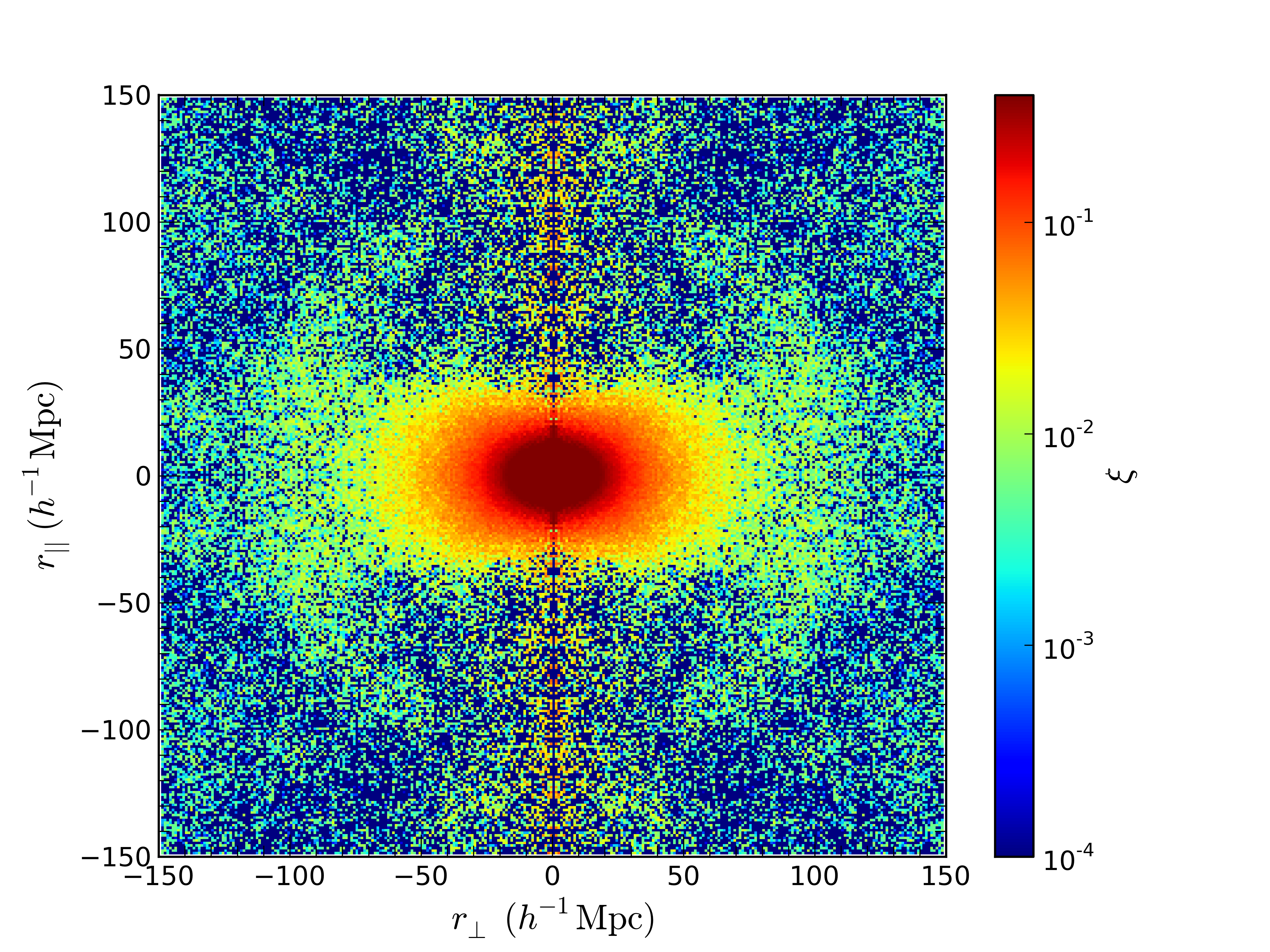
Fig. 2 shows the two-dimensional correlation function of DR11 sample measured in bins of . Both the ‘BAO ridge’ (a ring of local maxima at approximately 100 Mpc) and the RSD signal (LOS ‘squashing’ of the correlation function) are detectable by eye.
The random catalogue is constructed by populating the volume covered by galaxies with random points with zero correlation. We use a random catalogue that has 50 times the density of galaxies to eliminate extra uncertainty associated with the shot noise in the random catalogue.
We weight each galaxy in the catalogue with three independent weights. First is the Feldman–Kaiser–Peacock (FKP; Feldman, Kaiser & Peacock, 1994) weight . This approach downweights galaxies in high-density regions, achieving a balance between cosmic variance and shot-noise errors. The second weight accounts for the systematic effects associated with both the varying stellar density (; Ross et al., 2012) and seeing variations in the imaging catalogue used for targeting (; Anderson et al., 2014). The third weight corrects for the missed galaxies due to fibre collisions and redshift failures using the algorithm described in Anderson et al. (2012). The former is caused by the finite size of fibres that makes simultaneous measurement of spectra of two galaxies with small angular separation impossible. To correct for both of these effects, we upweight each galaxy by the number of its lost neighbours and the resulting weight is . Since these effects are statistically independent, the total weight is a product of three . The weight of the pair is the product of individual weights for two galaxies. Since the stellar and close-pair effects are absent in the random catalogue we apply only the FKP weight to them.
The observed correlation function is a function of two variables: we use , the distance between galaxies, and , the cosine of the angle between their connecting vector and the LOS. The optimal choice of binning for the correlation function measurements depends on two competing effects. Using small bin size retains more information, but since we estimate covariance matrices by computing a scatter of finite number of mock catalogues (see section 4), using more bins deteriorates the precision at which the elements of the covariance matrices can be estimated. Empirical tests performed on the mock catalogues suggest that the RSD signal is more or less insensitive to the binning choice, while the BAO measurements are optimal at Mpc (for details see Percival et al., 2014). We bin in 16 bins of Mpc in size in the range of and in 200 bins in , and estimate the correlation function on this two-dimensional grid. The information in the correlation function below is strongly contaminated by non-linear effects, and the scales above have low signal-to-noise ratio and contribute little information.
We compress the information in the two-dimensional correlation function by computing the Legendre multipoles with respect to by approximating the integral with a discrete sum:
| (7) | |||||
| (8) |
where is the Legendre polynomial of the order of .
In the subsequent analysis we only use the monopole () and the quadrupole () moments. The higher order moments contain significantly less information and are more difficult to model. (For the contribution of the higher order moments see e.g. Taruya, Saito & Nishimichi, 2011; Kazin, Sanchez & Blanton, 2012).
The RSD signal in the measured correlation function varies within the sample due to redshift evolution [via the redshift dependence of and ]. If we keep track of the redshift of individual galaxy pairs in equation (6), we effectively measure
| (9) |
where summation is over individual galaxy pairs contributing to counts, is the correlation function at mean redshift of that galaxy pair and is the product of the weights of individual galaxies in the ith pair. Thus our measurement is actually a weighted redshift-averaged correlation function. The evolving correlation function can be expanded into Taylor series in redshift around some value of :
| (10) |
Keeping only the first-order term, we find
| (11) |
and the second term disappears if we define
| (12) |
If the derivatives of the correlation function of second order and higher are small, the redshift averaged correlation function is equal to the correlation function at an ‘effective’ redshift given by equation (12).
The ‘effective’ redshift defined in equation (12) is a function of scale. We adopt , a value which is close to the computed from the catalogue to better than 1 per cent precision for all scales in the range Mpc. We checked that in our fiducial CDM cosmology the contribution from the higher order terms in equation (11) are indeed small for the expected theoretical variations in within the redshift range. We will therefore interpret our estimates as measurements of the correlation function at this effective redshift.
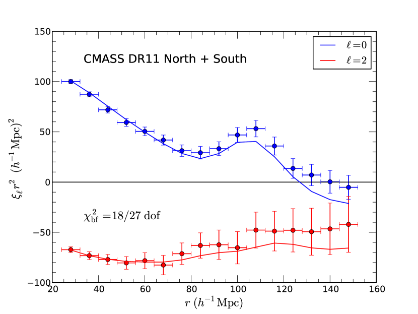
Fig. 3 shows the measured monopole and quadrupole of the CMASS galaxies along with errorbars (see section 4 for details of the error estimation). We will use these measurements in our analysis rather than the two-dimensional correlation function presented in Fig. 2.
4 The covariances
To estimate the covariance matrix of our measurements we use a suite of 600 PTHalo simulations. The simulations cover the same volume as the CMASS sample and are designed to produce a similar bias (for details of mock generation see Manera et al., 2013).
We compute the Legendre multipoles from each individual mock catalogue and estimate the covariance matrix as
| (13) |
where the sum is over individual mocks and the average multipoles
| (14) |
are also computed from the mocks. The unbiased estimator of the inverse covariance matrix is then given by
| (15) |
where 32 is the number of bins used in the analysis (for details see Percival et al., 2014). Fig. 4 shows the reduced covariance matrix (diagonal elements normalized to one) of our multipoles. As expected, the measured multipoles in the neighbouring -bins are strongly correlated. The correlation between measured monopole and quadrupole at the same scale is up to 15 per cent on smaller scales.

We will compute the likelihood of theoretical models as
| (16) |
where
| (17) |
are the set of parameters and are the theoretical predictions for the multipoles. In equation (17) we additionally rescale the inverse covariance matrix
| (18) | |||||
| (19) | |||||
| (20) |
where is the length of vector . This accounts for the uncertainties in the determination of the inverse covariance matrix from the finite number of catalogues (for details see Percival et al., 2014). In our case, , and , which results in and .222We use here even though the total number of fitted parameters is 8, because the three ‘shape’ parameters are constrained almost exclusively by the Planck covariance matrix of equation (29) which is not derived from our suite of 600 PTHalo mocks and is assumed to be exact. The multiplicative correction factor is then .
In approximating the likelihood by equations (16) and (17), we made two assumptions: that the errors on the monopole and quadrupole are drawn from a multivariate Gaussian distribution (equation 16) and that the dependence of inverse covariance matrix on free parameters is weaker than the dependence of the model [ in equation (17)].
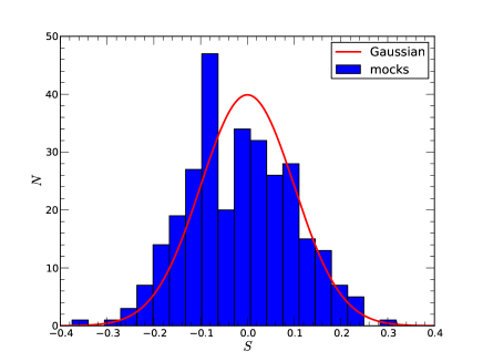
Non-linear evolution will induce non-Gaussianity. To check the validity of the first assumption, we estimate a skewness of in bins of from the 600 PTHalo mocks using
| (21) |
Fig. 5 shows a histogram of the resulting distribution of sample skewness and the prediction made assuming that the distribution of is Gaussian. The observed distribution is consistent with the assumption of Gaussianity; therefore, we will ignore the contribution of possible non-Gaussian contributions to the likelihood of .
The validity of our second assumption is helped by the fact that the signal-to-noise ratio is high and the mock catalogues were tuned to reproduce the observed clustering of CMASS sample on average (see Manera et al., 2013, for details).
5 Theoretical model
5.1 Modelling multipoles
We use the ‘streaming model’ to compute our theoretical template correlation function. Within the streaming paradigm the correlation function in redshift space is derived by taking a real space, isotropic correlation function and convolving it along the LOS with a probability distribution function of the infall velocity of a galaxy pair at that separation.
| (22) |
where and are the components of a vector in the parallel and perpendicular to the LOS direction; and are the analogous components in the real space. In the plane-parallel approximation we adopt here, . The function accounts for both quasilinear infall motions and the random small-scale velocities (‘Finger-of-God’ effect; Jackson, 1972).
Following Reid & White (2011), we assume
| (23) |
and compute the and values using the standard perturbation theory, while the correlation function in the configuration space – – is computed using Lagrangian perturbation theory (see Reid & White, 2011, for details). The parameter is an isotropic dispersion that accounts for motions of galaxies within their local environment that are approximately uncorrelated with the large-scale velocity field; this parameter is varied within a broad prior consistent with the expected contribution from satellite galaxies; see Reid et al. (2012) for further discussion.
Recently, Wang, Reid & White (2014) extended the results of convolution Lagrangian perturbation (Carlson, Reid & White, 2013) and combined them with the ‘streaming model’ to obtain accurate predictions for the two-dimensional correlation function. This improved model is accurate for a wider range of biases than the original model. For the CMASS sample, however, the original implementation of the model in Reid & White (2011) remains accurate enough and is used in this analysis (see also discussion following Fig. 6).
If the real geometry of the Universe differs from the fiducial cosmology used to compute the correlation function, this will result in the additional distortions via the AP effect. To account for this, we rescale the redshift-space correlation function in equation (23) as
| (24) |
where
| (25) |
and and are the Hubble expansion rate and the angular distance in the fiducial cosmology.333These parameters were incorrectly defined in the text of Reid et al. (2012), but implemented correctly.
The model correlation function depends on the growth rate via and . The higher values of result in higher amplitude of both multipoles. The dependence on the Hubble expansion rate and angular distance arise from the AP effect and are manifested as distortions of the multipole shapes.
Our model has been compared to N-body simulations and shown to fit the anisotropic clustering down to scales of Mpc with per cent level precision (Reid & White, 2011; Reid et al., 2012). To check that the PTHalo mocks adequately describe the RSD signature in the range of scales used in the analysis we fit our model to the mock measurements. For simplicity, we fix the shape of the linear power spectrum to the input value and use the input cosmology to compute radial and angular distances (this is equivalent to fixing ) so that the only free parameters are , and . Fig. 6 shows the distribution of maximum-likelihood (ML) values of and recovered from the mock catalogues. The systematic offset between the mean of the ML values for and the input value of the mocks is of the order of 1 per cent, and the scatter in the ML values (after appropriate rescaling as in Percival et al., 2014) is comparable to the errors produced in section 6. At least at the two-point level, this shows that the relevant systematic effects in the PTHalos mocks are much less than our measurement precision and can be safely ignored.
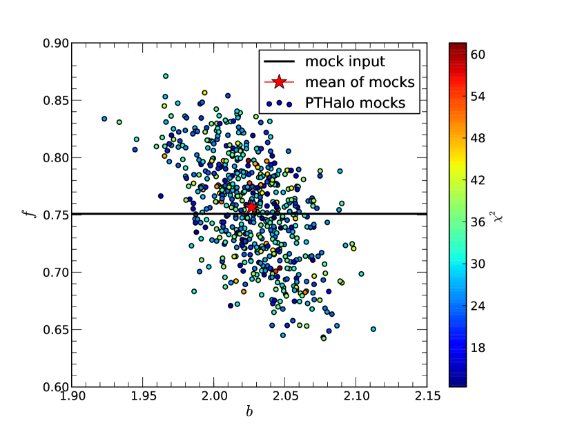
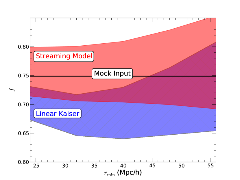
Fig. 7 shows the mean values and errorbars recovered by fitting individual PTHalo mocks with the non-linear ‘streaming model’ as a function of minimal scale used in the analysis. The figure also shows the results if we use a linear theory model (Kaiser, 1987) with no velocity dispersion nuisance parameter. We find that for the BOSS DR11 data, one would need to fit above Mpc to get unbiased estimates of the growth rate with the linear model. The non-linear model resulted in unbiased fits even when scales down to Mpc were used.
The model predictions for depend on eight parameters. These are parameters determining the shape of the linear correlation function , the bias of galaxies , the linear growth rate , two AP parameters and , and FOG velocity dispersion, . In linear theory, and are completely degenerate with , and observed clustering is only sensitive to their combination and . Even though non-linear effects break this degeneracy, it is still present to high degree. To compute non-linear effects on the real-space correlation function as well as mean and variance of infall velocity, we need to specify a value of . In our analysis, we fix the value of , which is the best-fitting value to Planck data within the CDM-GR model. We checked that model predictions do not change significantly if we keep the values of and fixed and vary within of the Planck constraints, and therefore, the recovered value of is not sensitive to the fiducial used to compute non-linear effects. When combining our measurements with Planck data to constrain cosmological models, we do not fix a value of and compute it for each model accordingly (see section 7).
5.2 Modelling DE and gravity
The large-scale properties of the Universe after inflation depend on several variables. First, we have the relative abundances of the main energy-density constituents – radiation , baryons , dark matter and DE . We must also specify the parameters describing initial conditions at the end of inflation – the spectral index and the amplitude of curvature perturbations . Finally, the behaviour of DE can be fully described by its effective equation of state (EoS) if the perturbations to DE fluid are negligible.
The energy density of radiation is determined with extremely high precision from the temperature of microwave background and is negligible at late times. In addition, the standard inflationary paradigm predicts the Universe to be spatially flat to a high degree, which means that the DE energy density can be expressed in terms of other components . The parameters , and are tightly constrained by CMB data in a way that is independent of late-time behaviour of DE and gravity. The CMB also provides a measurement of a distance, to the last-scattering surface which depends on DE, but since it utilizes only one integrated measurement of distance it results in highly degenerate constraints on and if used on its own.
The low-redshift measurements from anisotropic galaxy clustering are strongly complementary to CMB information. The quantities and depend on and DE properties, breaking degeneracies of CMB data. The in the measurement is sensitive to . Relating to in a given model provides a strong additional test of both DE and gravity. The fluctuations in the galaxy field ( measured by RSD) are a result of initial fluctuations at recombination ( measured by CMB), and their relationship depends on the strength of gravity and expansion of the Universe from to the redshift of the galaxy sample. Even small offsets from GR and are amplified and result in large offsets at low redshifts.
Independent probes of distance and expansion rate, such as measurements of luminosity distance from supernovae Type Ia (SNIa) or direct measurements of , further enhance the cosmological constraints.
6 Measurements
The measured monopole and quadrupole (see section 3) along with the covariance matrix estimated from PTHalo mocks (see section 4) are fitted with the predictions of the streaming model (see section 5) to derive constraints on the geometry and the growth rate at an effective redshift of .
The theoretical template for the multipoles depends on the parameters .
Constraints on the shape of the correlation function () from CMB data are significantly tighter than similar constraints obtainable from galaxy clustering only, and these constraints are largely independent of either the behaviour of DE at low redshifts or the nature of gravity (i.e. the values of , and which are of main interest here). To exploit this fact, we multiply the likelihood in equation (16) by a Planck prior on this triplet
| (26) |
with
| (27) |
and the mean values of and the are given by Planck temperature anisotropy data (Planck Collaboration, 2013). We use the shape prior derived from the combination of Planck temperature anisotropy data with the WMAP low-multipole polarization likelihood which is (Planck Collaboration, 2013)
| (28) | |||||
| (29) |
To explore this parameter space we use the nested sampling method as implemented in the multinest software package (Feroz, Hobson & Bridges, 2009; Feroz et al., 2013). The free parameters of the model and their priors are listed in Table 1.
| Parameter | Min. value | Max. value |
|---|---|---|
| 1.0 | 1.6 | |
| 0.0 | 1.0 | |
| 0.8 | 1.2 | |
| 0.8 | 1.2 | |
| 0.0 | 50.0 | |
| 0.08 | 0.14 | |
| 0.018 | 0.026 | |
| 0.8 | 1.2 |
We have checked a posteriori that this range includes all the high likelihood regions up to at least in all parameters except (see discussion in section 6.1). The resulting constraints on main cosmological parameters are presented in Table 2.
| Parameter | Central value | error |
|---|---|---|
| 1.29 | 0.03 | |
| 0.441 | 0.043 | |
| 1.006 | 0.033 | |
| 1.015 | 0.017 |
To derive constraints on DE and MG parameters we will be using the marginalised likelihood of parameters , and , where is the sound horizon scale at the drag epoch. This marginalized likelihood can be approximated as a Gaussian with mean
| (30) | |||||
and covariance matrix
| (31) |
Equations (30) and (31) use values of derived by numerically integrating the recombination equations and integrating the sound speed up to the drag epoch. These values are related to the results derived from commonly used fitting formula of Eisenstein & Hu (1998) adjusted by a factor of . This ratio is independent of cosmology for a wide range of conventional cosmological models (see e.g. Mehta et al., 2012).
Fig. 8 shows the constraints on main cosmological parameters compared to the expectations from the Planck data within standard CDM-GR models along with DR9 results from Reid et al. (2012). The DR11 results are in a good agreement with the Planck predictions; the difference between them is 1.6 for 3 degrees of freedom.

Equations (30) and (31) represent the main results of our work and will be used later to constrain models of DE and MG (see section 7).
6.1 Comparison to other similar measurements
The companion papers, Anderson et al. (2014), Beutler et al. (2013), Sanchez et al. (2014) and Chuang et al. (2013) use the same CMASS DR11 data to constrain the distance–redshift relation at .
Fig. 9 shows our measurement of distance along with the result from BAO only fits and previous similar measurements and Planck predictions for spatially-flat CDM model.
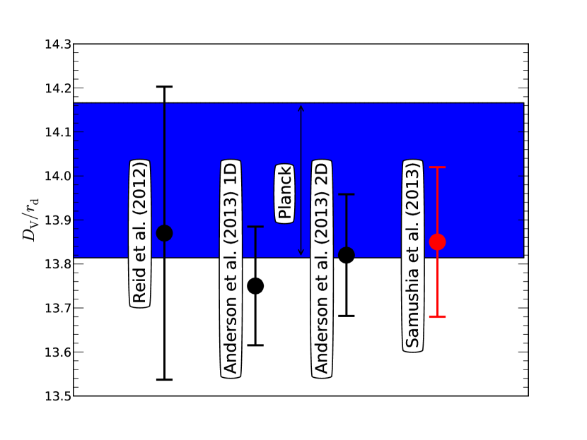
In Fig. 9, the label 1D refers to the result derived by fitting the monopole of the correlation function only, while the label 2D refers to the result derived from the fit to the monopole and the quadrupole of the correlation function (see Anderson et al., 2014, for details). differ from our analysis in two important aspects. They apply ‘reconstruction’ to the measured galaxy distribution to partially remove the nonlinear smearing of the BAO feature, and marginalize over the broad-band shape of the correlation function, so that the estimate of the distance comes from the BAO peak feature alone.
Beutler et al. (2013) and Chuang et al. (2013) measured the distance–redshift relationship using the Legandre moments of power spectrum and correlation function, respectively. Beutler et al. (2013) perform their analysis in Fourier space. The Chuang et al. (2013) analysis is in configuration space but uses a different range of scales and theoretical model than our work. Despite differences in the applied methodology, the estimates are consistent within 1 error bars.
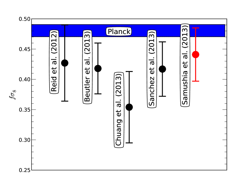
The growth rate, , has also been measured in the same redshift bin by Beutler et al. (2013, DR11), Reid et al. (2012, DR9), Chuang et al. (2013, DR11) and Sanchez et al. (2014). The comparison of results is presented in Fig. 10. In the Sanchez et al. (2014) analysis, is a derived parameter computed by combining CMASS data with Planck assuming CDM model; their estimate is perfectly consistent with ours. The Reid et al. (2012) analysis is similar in the range of scales and theoretical modelling to the current paper, but performed on DR9 data set. All measurements are consistent with each other and are somewhat lower than the Planck CDM-GR expectations.
6.1.1 Comparison with our DR9 measurements
The fitting methodology adopted in this paper is identical to that used in our DR9 analysis (Reid et al., 2012), but some of the priors have been updated. We adopt a prior on the linear matter power spectrum shape from Planck rather than WMAP7; Planck has substantially smaller errors, and so we expect the marginalization over the to contribute negligibly to our error budget in DR11. We also adopted a slightly more conservative top-hat prior on , by increasing the allowed range from 0 – 40 to 0 – 50, as the large-scale clustering data alone can-not well constrain this dispersion term; we have checked that this change of prior range does not affect our best-fitting parameter values significantly.
The effective area of DR11 is a factor of 2.5 larger than DR9; in the limit of negligible boundary effects, we would expect the covariance matrix on , and to be reduced by the same factor. A direct comparison indicates agreement at the level on the diagonals, with DR11 errors slightly larger than expected and with different off-diagonal structure. When projected on to (at fixed and ), which is the relevant case for the modified gravity constraints we present, our error in DR9 was 0.033 and is 0.028 in DR11, while we would have expected 0.021 from the effective volumes. This situation arises because, as we showed in table 2 of Reid et al. (2012), the prior on reduces the uncertainty on in the fixed geometry case substantially. The statistical errors have shrunk significantly in DR11, but we did not assume better prior knowledge on .
Fisher matrix analysis suggests that if parameter were perfectly known, the error would be reduced to 0.017 when the geometric and power spectrum parameters are held fixed.444For an update on the small-scale estimate and its effect on measurement see Reid et al. (2014).
In DR11 we obtain higher values for and , which brings us slightly closer to the values predicted by Planck. The offset between DR11 and DR9 results is just 0.3 per 3 degrees of freedom.
6.2 Constraints from monopole and quadrupole Separately
To determine the separate contribution of monopole and quadrupole we perform the same fit to each individually. The monopole and quadrupole measurements on their own are unable to break the degeneracy between and and can only constrain combinations of the two. Fig. 11 shows the constrains in – derived from the two multipoles. The solid lines show the expected degeneracy directions based on the linear theory predictions.
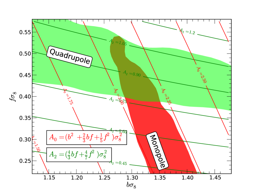
The quadrupole best constrains , as expected from the linear theory. The amplitude constraints from monopole are collinear to the combination , also as expected from linear theory.
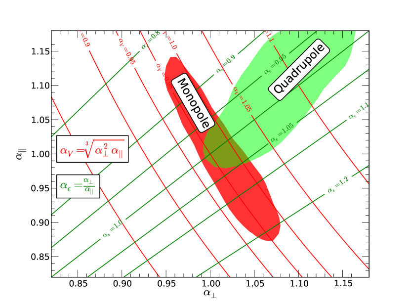
The AP parameters and show a qualitatively similar picture. Individual multipoles can only constrain certain combinations of parameters. Fig. 12 presents constraints in the – plane from the monopole and quadrupole separately. The solid lines show the expected degeneracy directions based on the linear theory predictions.
The principal component of the monopole constraint coincides with as expected from linear theory. The principal component of the quadrupole constraint is slightly tilted from the direction; from the monopole and from the quadrupole.
6.3 Separate fits to growth and AP
We next fit the monopole and quadrupole for the growth factor and AP parameters separately. First, we assume that the background expansion follows the predictions of spatially flat CDM but allows the growth rate to be a free parameter. In this case, the parameters and can be computed from and . For this model, where the background expansion is assumed to be following the CDM predictions, we find and . The constraint on growth improves to 6 per cent (from 10 per cent) and is perfectly consistent with the result of our more general fit.
Next, we assume that the growth rate follows the predictions of CDM-GR, but let the expansion rate and the distance–redshift relation vary. In this case is computed from but the and are free parameters. For this fit, we obtain and . Constraints on move to a lower value and tighten to 2 per cent (from 3 per cent), while constraints on move to a higher value and tighten to 1 per cent (from 2 per cent).
6.4 Contribution from small scales
Moments of the correlation function are measured with the best signal-to-noise ratio at small scales. The model that we use has been tested against numerical simulations with agreement at the per cent level down to Mpc. To determine explicitly the contribution of small scales on our fits, we redo the fit to the monopole and quadrupole keeping only scales above Mpc. The results of this fit and the comparison to the main results are shown in Fig. 13.
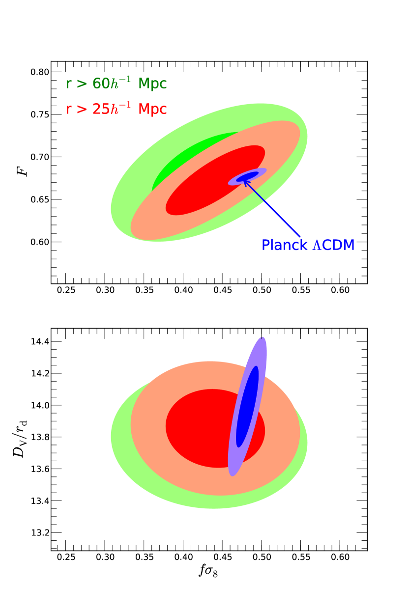
The inclusion of scales between Mpc improves our constraints by approximately a factor of 2. For the main parameters of interest we find , , , and . The biggest improvement is in the variables that are determined from the amplitudes of the multipoles such as , and . Improvement in is more modest, because most of the information about this quantity is produced by the BAO peak in the monopole at Mpc.
Small-scale clustering pushes and to higher values and to lower values. The two estimates, however, are highly consistent, the offset between the two being for 3 degrees of freedom. Both sets of measurements are consistent with Planck data. The difference between large-scale-only measurements and Planck inferred values is 1.8 for 3 degrees of freedom, while the difference between large-scale-only measurements and the ones using all scales above 25 Mpc is 0.3 for 3 degrees of freedom.
7 Cosmological implications
In following subsections, we constrain parameters of standard CDM-GR model by combining our measurements with the CMB and previous, independent BAO measurements. We also examine possible deviations from the standard model by considering phenomenological modifications to both and GR parts.
As a CMB data set we adopt the recent measurements of CMB temperature fluctuations by the Planck satellite (Planck Collaboration, 2013) supplemented by low- measurements of CMB polarization from the WMAP misssion (Bennet et al., 2013) and the high- measurements from the Atacama Cosmology Telescope (Das et al., 2013, ACT) and the South Pole Telescope (Reichart et al., 2012, SPT). For the rest of the paper, we will refer to this combination of CMB data as ePlanck555When computing the CMB likelihood we make the same assumptions as Planck Collaboration (2013). For example, we assume a minimum neutrino mass of . This affects the time of matter-radiation equality and angular-diameter distance to last scattering, as well as early integrated Sachs–Wolfe effect and the lensing potential.. For our BAO data compilation we use measurements from Beutler et al. (2011, ), Anderson et al. (2014, )666We only use a measurement of BAO from the lower redshift (LOWZ) sample since the measurement from the CMASS sample is highly correlated with our own estimate of . and Blake et al. (2011a, ).
To sample cosmological parameter space, we use the Monte Carlo Markov Chain (MCMC) technique implemented by the cosmomc package (Lewis & Bridle, 2002).
7.1 CDM-GR
In a spatially flat CDM-GR model, the expansion history of the Universe and the growth of perturbations can be fully described by six parameters. We choose these to be . The mean values and 1 confidence levels are listed in Table 3.
| CDM-GR | |||
|---|---|---|---|
| Parameter | ePlanck | BOSS + ePlanck | BOSS + ePlanck + BAO |
By combining BOSS DR11 results with Planck data, we are able to achieve a 1.6 per cent constraint on , a 1.3 per cent constraint on and a 1.2 per cent constraint on . After including BAO data set, the constraints improve to 1.3 per cent on and a 1.0 per cent constraint on , while relative constraint on does not change. The constraints on and are dominated by the information from the ePlanck data set.
7.2 Spatial curvature
We now relax the assumption that the spatial curvature is zero and allow the parameter to vary along with . The posterior confidence regions on curvature and nonrelativistic matter density are shown in Fig. 14.
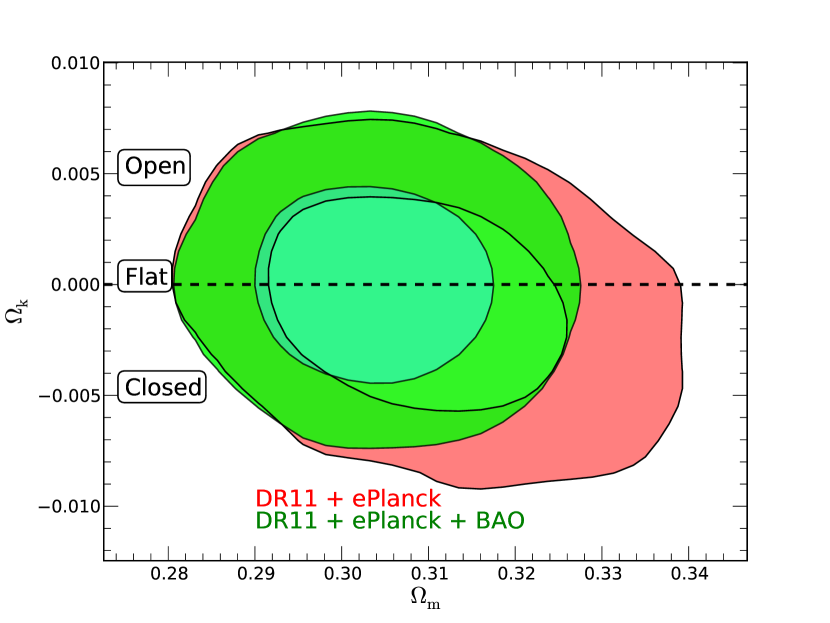
We find (a 0.3 per cent constraint) when combining BOSS DR11 with ePlanck and (a 0.3 per cent constraint) when adding the BAO compilation. In both cases the results are perfectly consistent with a spatially flat Universe.
7.3 Time dependence of DE
Alternative models of DE predict a time-dependent EoS . For a wide range of DE models that do not exhibit sudden transitions or large amount of DE at early times, for example models based on cosmological scalar fields, this time-dependence can be adequately parametrized by two parameters
| (32) |
(Chevallier & Polarski, 2001; Linder, 2003). (For DE models that do not belong to this family see e.g. Wetterich, 2004; Doran & Robbers, 2006). This reduces to our standard model for and .
We first set to zero and check if there is an evidence for to differ from on average. The confidence level contours on and nonrelativistic matter density are shown in Fig. 15.
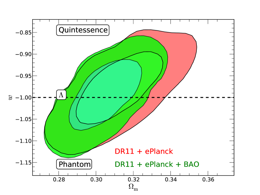
This analysis yields (a 8 per cent constraint) when BOSS DR11 is combined with ePlanck data and (a 6 per cent constraint) when the BAO compilation is added. In both cases, the results are perfectly consistent with a cosmological constant (). Our constraints on differ significantly from the DR9 results presented in Samushia et al. (2013), where we detected up to preference for . This change is mainly due to two differences. We now use ePlanck as our CMB data set, which predicts a higher value for the non-relativistic matter density. Also, our new measurements, although consistent with DR9 results, have moved in the direction that makes them more consistent with the CMB results (see Fig.8).
Finally, we consider a model in which the spatial curvature is a free parameter and both and are allowed to vary. The constraints on this model are shown in Fig. 16.
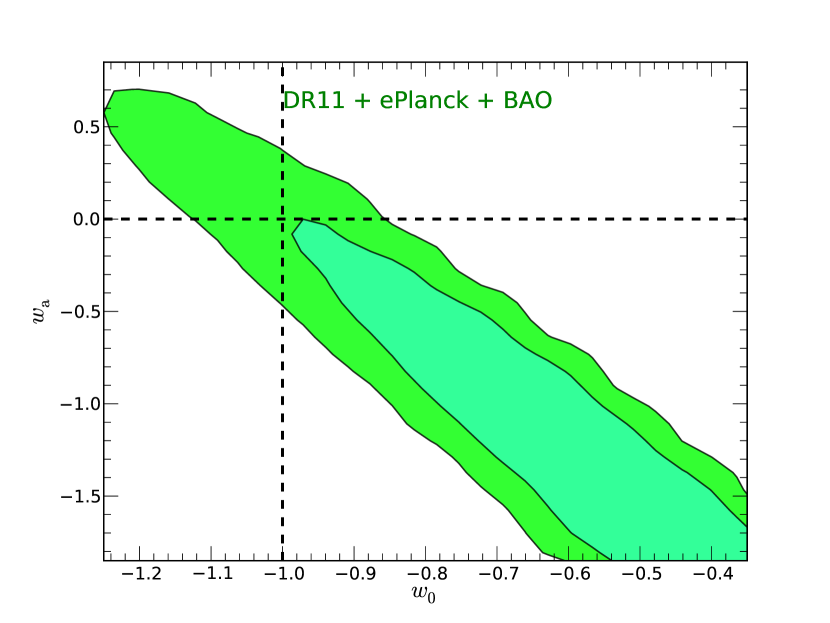
The DR11 data alone, even after combining with ePlanck, is not able to break all the degeneracies of this large parameter space. When DR11 and ePlanck are combined with the BAO, we see a preference for larger values of and smaller values of . The CDM value of and , however, is still within the confidence level.
7.4 Deviations from GR
MG predict scale dependence of bias and growth rate even in the linear regime and the effect of small-scale screening mechanisms is difficult to model. This makes devising a completely self-consistent test of MG models a non-trivial task. A number of proposals for parametrizing families of MG models have been discussed recently (see e.g. Battye & Pearson, 2012; Bloomfield et al., 2012; Baker, Ferreira & Skordis, 2013; Mueller, Bean & Watson, 2013). These parametrizations, however, are difficult to correctly implement in practice for a few reasons. First, they rely on the linear theory and are not expected to work below scales of Mpc. Secondly, they require a large number of free parameters and such a large parameter space cannot be effectively constrained by current data. For these reasons, we follow the approach of Samushia et al. (2013) and apply several few-parameter consistency tests to our measurements.
We parametrize the growth rate as a function of using
| (33) |
(Linder & Cahn, 2008). This approach does not provide a fully self-consistent test of MG models, as MG models predict a more complex change in observables compared to GR. This parametrization is, however, easy to implement and provides a simple consistency test. In GR, we expect the -index to be equal to 0.554. Measuring a significantly higher value would indicate a preference for a force weaker than GR gravity and vice versa. In our fits, we apply a hard prior of .
When constraining deviations from GR, we fix DE to be a cosmological constant. We also ignore the CMB power spectrum on large scales () to ensure that CMB data are used only to constrain the background evolution. The parametrizations that we use are not physically motivated and are simply meant to describe effective gravity at low redshifts rather than provide a full model that works accurately at all redshifts up to last-scattering surface.
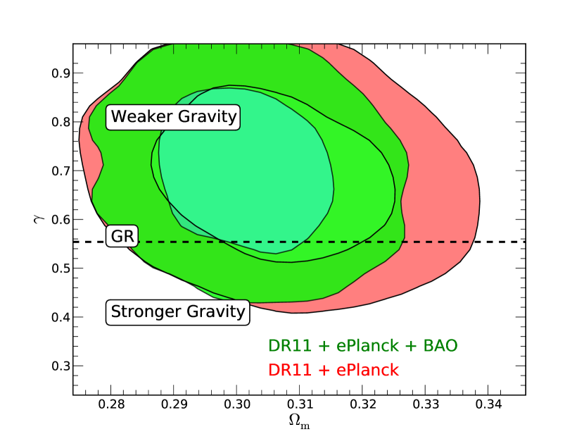
Constraints on and are shown in Fig. 17. When combining BOSS DR11 with ePlanck data, we recover (a 16 per cent measurement). With the BAO data set, we recover (a 16 per cent measurement). The values are within confidence of GR values but favour a weaker gravity.
Next, we parametrize the linear equation of growth following the approach of Pogosian et al. (2010) as
| (34) |
where is a matter overdensity, the overdot denotes a derivative with respect to , is the gravitational constant, and and are parameters describing deviations from GR. The GR limit is recovered when , where negative values of correspond to weaker than GR gravity and vice versa. The parameter dictates how rapidly the modifications are set larger values of corresponding to the modifications that appear at later times. Since large values of correspond to models in which gravity is indistinguishable from GR until some low redshift when the modification suddenly becomes significant, they are basically unconstrained. We place a flat prior of to avoid this problem. The confidence level contours of and are shown in Fig. 18.
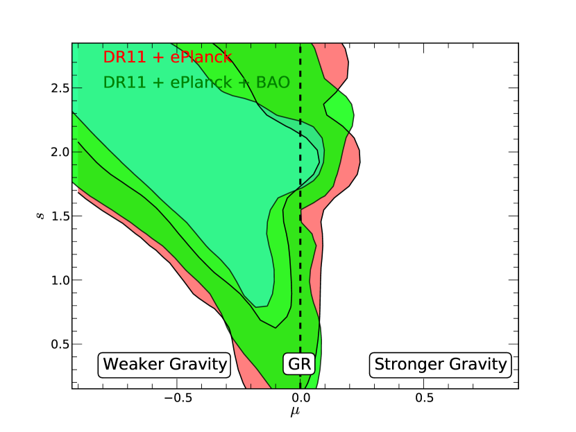
The GR predictions are within in posterior likelihood. Similar to -parametrization, the data again provide a mild preference for a weaker than GR gravity. This result is consistent with the DR9-based results reported in Samushia et al. (2013).
8 Conclusions
We have used the anisotropic clustering of galaxies in the BOSS DR11 data set to simultaneously constrain the growth rate, the redshift–distance relationship and the expansion rate at the redshift of . Overall, our measurements are in good agreement with the results of the Planck satellite propagated to low redshifts assuming CDM-GR.
By combining our measurements of , and with the CMB data we were able to derive tight constraints on basic cosmological parameters and parameters describing deviations from the CDM-GR model. We were able to constrain the curvature of Universe with 0.3 per cent precision, the DE EoS parameter with 8 per cent precision and the -index for growth with 16 per cent precision.
When we vary the background expansion within CDM predictions of the Planck data we measure the growth rate (parametrized by ) to be weaker but consistent within of GR predictions. This preference for lower values of growth rate has also been observed in other similar low-redshift measurements (see e.g. Macaulay, Wehus & Eriksen, 2013, for discussion). Our measurement of follows this trend but is closer to the GR predictions compared to the DR9 results of Reid et al. (2012) and the DR11 measurement of Beutler et al. (2013).
Similar measurements from a lower redshift (LOWZ) sample of BOSS galaxies will provide a complementary measurement of the growth rate in the DE-dominated redshift range of , which will significantly strengthen the constraining power over possible GR modifications and can potentially increase the significance of the ‘low growth rate’ signal.
Acknowledgements
LS gratefully acknowledges support by the European Research Council. BAR gratefully acknowledges support provided by NASA through Hubble Fellowship grant 51280 awarded by the Space Telescope Science Institute, which is operated by the Association of Universities for Research in Astronomy, Inc., for NASA, under contract NAS 5-26555. Funding for SDSS-III has been provided by the Alfred P. Sloan Foundation, the Participating Institutions, the National Sci- ence Foundation, and the U.S. Department of Energy Office of Sci- ence. The SDSS-III web site is http://www.sdss3.org/.
SDSS-III is managed by the Astrophysical Research Consortium for the Participating Institutions of the SDSS-III Collaboration including the University of Arizona, the Brazilian Participation Group, Brookhaven National Laboratory, University of Cambridge, CarnegieMellon University, University of Florida, the French Participation Group, the German Participation Group, Harvard University, the Instituto de Astrofisica de Canarias, theMichigan State/Notre Dame/JINA Participation Group, Johns Hopkins University, Lawrence Berkeley National Laboratory, Max Planck Institute for Astrophysics, Max Planck Institute for Extraterrestrial Physics, New Mexico State University, New York University, Ohio State University, Pennsylvania State University, University of Portsmouth, Princeton University, the Spanish ParticipationGroup, University of Tokyo, University of Utah, Vanderbilt University, University of Virginia, University of Washington, and Yale University.
We acknowledge the use of MCMC data from Planck Legacy Archive
(http://www.sciops.esa.int/index.php?project=planck&page=Planck_Legacy_Archive).
Numerical computations were done on the Sciama High Performance Compute cluster which is supported by the ICG, SEPNet and the University of Portsmouth.
References
- Albrecht et al. (2009) Albrecht A. et al., 2009, Findings of the Joint Dark Energy Mission Figure of Merit Science Working Group, arXiv:0901.0721 [astro-ph.IM]
- Alcock & Paczynski (1979) Alcock C., Paczynski B., 1979, Nature, 281, 358
- Anderson et al. (2012) Anderson L. et al., 2012, MNRAS, 427, 3435
- Anderson et al. (2014) Anderson L. et al., 2014, MNRAS, 441, 24
- Baker, Ferreira & Skordis (2013) Baker T., Ferreira P.G., Skordis C., 2013, PRD, 87, 024015
- Ballinger, Peacock & Heavens (1996) Ballinger W.E., Peacock J.A., Heavens A.F., 1996, MNRAS, 282, 877
- Bassett & Hlozek (2010) Bassett B.A., Hlozek R., 2010, in Ruiz-Lapuente P., ed., Dark Energy: Observational and Theoretical Approaches, Cambridge University Press, Cambridge, p. 246, arXiv:0910.5224 [astro-ph.CO]
- Battye & Pearson (2012) Battye R.A., Pearson J.A., 2012, JCAP, 7, 019
- Bennet et al. (2013) Bennet C.L. et al., 2013, ApJS, 208, 20
- Beutler et al. (2011) Beutler F. et al., 2011, MNRAS, 416, 3017
- Beutler et al. (2012) Beutler F. et al., 2012, MNRAS, 423, 3430
- Beutler et al. (2013) Beutler F. et al., 2013, MNRAS, 429, 3604
- Bianchi et al. (2012) Bianchi D. et al., 2012, 427, 2420
- Blake et al. (2011a) Blake C., Kazin E.A., Beutler F., Davis T.M., 2011, MNRAS, 418, 1707
- Blake et al. (2011b) Blake C., Brough S., Colless M., Contreras C., 2011, MNRAS, 415, 2876
- Blake et al. (2012) Blake C., Brough S., Colless M., Contreras C., 2012, 425, 405
- Bloomfield et al. (2012) Bloomfield J.K, Flanagan E.E., Park M., Watson S., 2012, preprint, arXiv:1211.7054 [astro-ph.CO]
- Bolton et al. (2012) Bolton A. et al., 2012, AJ, 144, 144
- Carlson, Reid & White (2013) Carlson J., Reid B.A., White M., 2013, MNRAS, 429, 1674
- Chuang & Wang (2013) Chuang C.-H., Wang Y., 2013, MNRAS, 431, 2634
- Chuang et al. (2012) Chuang C.-H. et al., 2012, MNRAS, 2013, 433, 3559
- Chuang et al. (2013) Chuang C.-H. et al., 2013, submitted to MNRAS, arXiv:1312.4889 [astro-ph.CO]
- Crocce, Scoccimarro & Bernardeau (2012) Crocce M., Scoccimarro R., Bernardeau F., 2012, MNRAS, 427, 2537
- Chevallier & Polarski (2001) Chevallier M., Polarski D., 2001, IJMPD, 10, 213
- Das et al. (2013) Das S. et al., 2013, preprint, arxiv:1301.1037 [astro-ph.CO]
- Dawson et al. (2013) Dawson K. et al., 2013, AJ, 145, 10
- Doran & Robbers (2006) Doran M., Robbers G., 2006, JCAP, 0606, 026
- Eisenstein & Hu (1998) Eisenstein D.J., Hu W., 1998, ApJ, 496, 605
- Eisenstein, Seo & White (2007) Eisenstein D.J., Seo H.-J., White M., 2007, ApJ, 664, 660
- Eisenstein et al. (2011) Eisenstein D.J. et al., 2011, AJ, 142, 72
- Elia et al. (2011) Elia A., Kulkarni S., Porciani C., Pietroni M., Matarrese S., 2011, MNRAS, 116, 1703
- Feldman, Kaiser & Peacock (1994) Feldman H.A., Kaiser N., Peacock J.A., 1994, ApJ, 426, 23
- Feroz, Hobson & Bridges (2009) Feroz F., Hobson M.P., Bridges M., 2009, MNRAS, 398, 1601
- Feroz et al. (2013) Feroz M., Hobson M.P., Cameron E.,Pettitt A.N., 2013, preprint, arXiv:1306.2144 [astro-ph.CO]
- Fukugita et al. (1996) Fukugita, M. et al., 1996, AJ, 111, 1748
- Gil-Marin et al. (2012) Gil-Marin H., Wagner C., Verde L., Porcini C., Jimenez R., JCAP, 11, 029
- Gunn et al. (2006) Gunn J.E. et al., 2006, AJ., 116, 3040
- Gunn et al. (2013) Gunn J.E. et al., 2013, AJ, 126, 32
- Guzzo et al. (2008) Guzzo L. et al., 2008, Nature, 451, 541
- Hamilton (1998) Hamilton A.J.S., 1998, preprint, arXiv:astro-ph/9708102
- Jackson (1972) Jackson J.C., 1972, MNRAS, 156, 1
- Kazin, Sanchez & Blanton (2012) Kazin E.A., Sanchez A.G., Blanton M.R., 2012, MNRAS, 419, 3223
- Sanchez et al. (2013a) Sanchez A. et al., 2013, MNRAS, 433, 1202
- Sanchez et al. (2014) Sanchez A. et al., 2014, MNRAS, 440, 2692
- Kaiser (1987) Kaiser N., 1987, MNRAS, 227, 1
- Landy & Szalay (1993) Landy S.D., Szalay A.S., 1993, ApJ, 412, 64
- Lewis & Bridle (2002) Lewis A., Bridle S., 2001, PRD, 66, 103511
- Linder (2003) Linder E.V., 2003, PRL, 90, 091
- Linder & Cahn (2008) Linder E.V., Cahn R.N., 2008, ApP, 28, 481
- Macaulay, Wehus & Eriksen (2013) Macaulay E., Wehus I.K., Eirksen H.K., 2013, PRL, 111, 161301
- Manera et al. (2013) Manera M. et al., MNRAS 2013, 428, 1036
- Marulli et al. (2012) Marulli F., Bianchi D., Branchini E., Guzzo L., Moscardini L., Angulo R.E., MNRAS, 2012, 426, 2566
- Mehta et al. (2012) Mehta K.T., Cuesta A.J., Xiaoying X., Eisenstein D.J., Padmanabhan N., MNRAS, 2012, 427, 2168
- Meiksin, White & Peacock (1999) Meiksin A., White M., Peacock J.A., 1999, MMRAS, 304, 851
- Mueller, Bean & Watson (2013) Mueller E.-M., Bean R., Watson S., 2013, PRD, 87, 083504
- Okamura, Taruya & Matsubara (2011) Okamura T., Taruya A., Matsubara T., 2011, JCAP, 8, 12
- Padmanabhan et al. (2012) Padmanabhan N. et al., 2012, MNRAS, 427, 2132
- Percival et al. (2014) Percival W.J. et al., 2014, MNRAS, 439, 2531
- Planck Collaboration (2013) Planck Collaboration, 2013, preprint, arXiv:1303.5076 [astro-ph.CO]
- Pogosian et al. (2010) Pogosian L., Silvestri A., Koyama K., Zhao G.-B., 2010, PRD, 81, 104023
- Rapetti et al. (2013) Rapetti D. et al., 2013, MNRAS, 432, 973
- Reichart et al. (2012) Reichart C.L., Shaw L., Zahn O., 2012, ApJ, 755, 23
- Reid & White (2011) Reid B.A., White M., 2011, MNRAS, 417, 1913
- Reid et al. (2012) Reid B.A. et al., 2012, MNRAS, 426, 2719
- Reid et al. (2014) Reid B.A. et al., 2014, preprint, arXiv:1404.3742 [astro-ph.CO]
- Ross et al. (2012) Ross A.J. et al., 2012, MNRAS, 424, 564
- Ross et al. (2014) Ross A.J. et al., 2014, 437, 1109
- Samushia et al. (2011) Samushia L. et al., 2011, MNRAS, 410, 1993
- Samushia, Percival & Raccanelli (2012) Samushia L., Percival W.J., Raccanelli A., 2012, MNRAS, 420, 2102
- Samushia et al. (2013) Samushia L. et al., 2013, MNRAS, 429, 1514
- Simpson et al. (2013) Simpson F. et al., 2013, MNRAS, 429, 2249
- Smee et al. (2013) Smee S.A. et al., 2013, AJ, 126, 32
- Strateva et al. (2001) Strateva I. et al., 2001, AJ, 122, 1861
- Taruya, Nishimichi & Saito (2010) Taruya A., Nishimichi T., Saito S., 2010, PRD, 82, 063522
- Taruya, Saito & Nishimichi (2011) Taruya A., Saito S., Nishimichi T., 2011, 83, 103527
- de la Torre & Guzzo (2012) de la Torre S., Guzzo G., 2012, MNRAS, 427, 327
- de la Torre et al. (2013) de la Torre S. et al., 2013, A&A, 557, 54
- Vlah et al. (2012) Vlah Z., Seljak U., McDonald P., Okamura T., Baldauf T., 2012, JCAP, 11, 009
- Wang, Reid & White (2014) Wang L., Reid B.A., White M., 2013, MNRAS, 437, 588
- Weinberg et al. (2013) Weinberg D.H., Mortonson M.J., Eisenstein D.J., Hirata C., Reiss A.G., Eduardo R., 2013, Phys. Rep., 530, 87
- Wetterich (2004) Wetterich C., 2004, PLB, 594, 17
- Zhao et al. (2012) Zhao G.-B. et al., 2012, PRD, 85, 123546
Appendix A CMB shape prior
Figure 19 displays the posterior likelihood of obtainable from DR11 data alone.
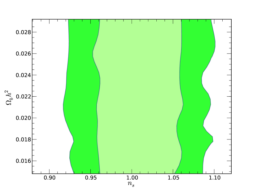
The likelihood surface does not close even within of the CMB constraints. Previous studies either fix the shape parameters to their CMB best-fit values (e.g. Samushia, Percival & Raccanelli, 2012), let vary and fix the rest (e.g. Blake et al., 2011b) , or marginalise over them by taking a prior centered around CMB best-fit values (e.g. Chuang et al., 2012).
We adopt a different approach and apply the CMB shape prior to our galaxy clustering likelihood. Since later we will combine our results with Planck data to obtain constraints on DE and MG parameters one may be led to an erroneous impression that the CMB data is being double-counted. We demonstrate below that this is not the case.
Let be a CMB likelihood, where are shape parameters and are other parameters that may be related to DE and gravity parameters of interest []. Let be galaxy likelihood, where are DE and gravity dependent []. For simplicity, assume , and to be scalars and that all likelihoods are multivariate Gaussian.
In our approach we take a CMB shape prior
| (35) |
apply it to galaxy data
| (36) |
and then combine it with full CMB likelihood
| (37) |
where .
Let’s compare this expression to that produced by directly combining the two likelihoods
| (38) |
and are also Gaussian with
| (39) | |||||
| (40) | |||||
| (41) |
always encloses . To first order in
| (42) | |||||
| (43) | |||||
| (44) |
| (45) | |||||
| (46) | |||||
| (47) |
This demonstrates that direct combination of galaxy clustering and CMB data always produce stronger constraints on derived parameters and therefore the galaxy clustering measurements obtained by assuming a CMB prior on the shape can be combined with the CMB data without double counting the information.
