Two-state thermodynamics of the ST2 model for supercooled water

Abstract

Thermodynamic properties of the ST2 model for supercooled liquid water exhibit anomalies similar to those observed in real water. A possible explanation of these anomalies is the existence of a metastable, liquid–liquid transition terminated by a critical point. This phenomenon, whose possible existence in real water is the subject of much current experimental work, has been unambiguously demonstrated for this particular model by most recent simulations. In this work, we reproduce the anomalies of two versions of the ST2 model with an equation of state describing water as a non-ideal “mixture” of two different types of local molecular order. We show that the liquid–liquid transition in the ST2 water is energy-driven. This is in contrast to another popular model, mW, in which non-ideality in mixing of two alternative local molecular orders is entropy-driven, and is not sufficiently strong to induce a liquid–liquid transition.

I Introduction

Liquid water is still poorly understood. Unlike ordinary substances, cold liquid water (near the triple point and, especially, in the supercooled region) and high-temperature liquid water behave as differently as if they consisted of different molecules. Highly-compressible, low-dielectric-constant water at high temperatures is a good solvent for hydrocarbons. On the low-temperature side of the phase diagram, water is an almost incompressible, high-dielectric-constant liquid, a good solvent for electrolytes, and exhibits numerous anomalous properties. The most famous anomaly is the maximum of the density at 4 °C. Even more striking is the anomalous behavior of water’s thermodynamic response functions, such the heat capacity,Angell, Shuppert, and Tucker (1973); Angell, Oguni, and Sichina (1982); Tombari, Ferrari, and Salvetti (1999); Archer and Carter (2000) compressibility,Speedy and Angell (1976); Kanno and Angell (1979); Mishima (2010a) and thermal expansivity,Hare and Sorensen (1987); Kanno and Angell (1980); Ter Minassian, Pruzan, and Soulard (1981) which becomes significantly more pronounced in the metastable supercooled state, suggesting a possible divergence at a temperature just below the homogeneous ice nucleation limit. One of the scenarios formulated to explain the anomalous behavior of water is the existence of a liquid–liquid transition terminated by a liquid–liquid critical point.Poole et al. (1992); Mishima and Stanley (1998a); Stanley et al. (2000); Stokely et al. (2010) The existence of the liquid–liquid transition in water, the so-called liquid water polyamorphism,Tanaka (2000); Mishima (2010b) has remained a fascinating, but highly debated, hypothesis. Indirect experimental evidence that supports this scenario comes from the observation of kinks in the melting curves of metastable ice polymorphs.Mishima and Stanley (1998b); Mishima (2000, 2011) More recently, it has been shown that water possesses two glass transitions,Amann-Winkel et al. (2013) an important observation that is consistent with the existence of two different forms of liquid water. However, the liquid–liquid separation in bulk water has not yet been directly observed in experiment, because of the challenge posed by rapid ice formation. The formation of ice can, in principle, be avoided on the time scales accessible with simulations of water-like models, allowing the properties of such models to be investigated under deeply supercooled conditions, thus providing additional insights into the nature of water’s anomalies. However, the existence of a liquid–liquid transition in a given water-like model is sensitive to the details of the intermolecular interactions. Furthermore, numerical artifacts associated with the implementation of simulation techniques can mask its presence.General Discussion (2013)

There are two popular models for water that demonstrate similar thermodynamic anomalies in the supercooled region but strikingly different phase behavior, ST2 and mW. In the ST2 model, each water molecule is comprised of five interaction sites arranged in a tetrahedral geometry.Stillinger and Rahman (1974) The ST2 model qualitatively reproduces many of the anomalous properties observed in real water. Its over-structured tetrahedral order enables one to study the anomalies at higher temperatures than for other models. As a result, ST2 has been used frequently in the computational investigations of water’s possible polyamorphism. Most simulations of the ST2 model have demonstrated the existence of the liquid–liquid separation in the supercooled region.Liu, Panagiotopoulos, and Debenedetti (2009); Sciortino, Saika-Voivod, and Poole (2011); Liu et al. (2012); Kesselring et al. (2012, 2013); Cuthbertson and Poole (2011); Poole et al. (2013); Palmer, Car, and Debenedetti (2013) Liu et al. Liu et al. (2012) observed two distinct liquid basins in the reversible free energy surface generated by computing, for a given temperature and pressure, histograms of density and an order parameter that distinguishes crystalline from amorphous configurations.Steinhardt, Nelson, and Ronchetti (1983) Poole et al. Poole et al. (2013) used a similar computational approach to perform an analysis for ST2 water modeled with the reaction-field treatment of the long-ranged electrostatics. The findings of Liu et al. Liu et al. (2012) and Poole et al. Poole et al. (2013) are also consistent with recent molecular dynamics simulations of ST2 water by Kesselring et al.,Kesselring et al. (2012) which show so-called “phase flipping” between the high-density liquid and low-density liquid on microsecond time scales. However, Limmer and ChandlerLimmer and Chandler (2011, 2013) in their simulations of the ST2 model observed only two minima in the free energy surface, one corresponding to a high-density liquid and the other to a low-density ice. They argued that the liquid–liquid transition in ST2 water, reported by other authors, was actually a liquid–crystal transition. The origin of the differences between the result of Limmer and Chandler and virtually all other studies of the ST2 model is still incompletely understood and is currently under investigation.General Discussion (2013) We also note the recent work by English et al.,English, Kusalik, and Tse (2013) who reported that the interface between the coexisting low- and high-density liquids is not stable. This result is in contrast with ongoing explicit interface simulation results in two of our groups, which will be the subject of a future publication.

Another interesting model of water is the mW model devised by Molinero and Moore.Molinero and Moore (2009) The mW model, suitable for fast computations, is a monatomic model of water; it models the water molecule as a single atom with only short-range interactions. The mW model imitates the anomalous behavior of cold and supercooled water, including the density maximum and the strong increase of the heat capacity and compressibility in the supercooled region.Molinero and Moore (2009); Moore and Molinero (2011); Limmer and Chandler (2011) Limmer and ChandlerLimmer and Chandler (2011, 2013) have shown that the mW model does not exhibit liquid–liquid separation in the range studied (from 0 MPa to 1000 MPa, down to 160 K). Indeed, Moore and MolineroMoore and Molinero (2011) demonstrated that in this model the supercooled liquid can no longer be equilibrated before it crystallizes and there is no sign of a liquid–liquid transition in the supercooled regime.

Despite the obvious difference with respect to the existence of the metastable liquid–liquid phase transition, one remarkable feature is shared by both ST2 and mW models,Cuthbertson and Poole (2011); Moore and Molinero (2009) and also possibly by real water:Nilsson, Huang, and Pettersson (2012); Taschin et al. (2013) the existence of two alternative, but interconvertible, configurations (or “states”) of local molecular order, namely a high-density liquid structure and a low-density liquid structure. A bimodal inherent structure in simulated TIP4P/2005 liquid water was also found by Wikfeldt et al. Wikfeldt, Nilsson, and Pettersson (2011) Competition between these configurations naturally explains the density anomaly and other thermodynamic anomalies in cold water. In particular, if the excess Gibbs energy of mixing of these two states is positive, the nonideality of the “mixture” can be sufficient to cause liquid–liquid separation, or, at least, to significantly reduce the stability of the homogeneous liquid phase and consequently generate the anomalies in the thermodynamic response functions. The best, so far, description of all currently available experimental data on thermodynamic properties of supercooled water is achieved with an equation of state based on the hypothesis of non-ideal, nearly athermal mixing of the two structures in water.Holten and Anisimov (2012a) However, since experimental data are not yet available beyond the homogeneous ice nucleation limit, the possibility of a liquid–liquid transition in real water must be examined by indirect means. The transition line is obtained from the extrapolation of the properties far away from the transition, thus making the location of the critical point very uncertain. The existence of a bimodal distribution of molecular configurations in water is supported by X-ray absorption and emission spectroscopyNilsson, Huang, and Pettersson (2012); Tokushima et al. (2008); Wernet et al. (2004) and an investigation of vibrational dynamics,Taschin et al. (2013) and there is information on the fraction of water molecules involved in each alternative structure.Wernet et al. (2004); Huang et al. (2009); Xu et al. (2009) Information on this fraction is also readily obtained from numerical or analytical calculations for water models. The fractions of molecules involved in the high-density structure and in the low-density structure at various temperatures and pressures were computed and reported by Moore and MolineroMoore and Molinero (2009) for the mW model, by Cuthbertson and PooleCuthbertson and Poole (2011) for the ST2 model, and by Wikfeldt et al. Wikfeldt, Nilsson, and Pettersson (2011) for the TIP4P/2005 model.

In this paper, we reproduce the anomalies of two versions of the ST2 model with an equation of state describing water as a non-ideal “mixture” of two different types of local molecular order. We show that the liquid–liquid transition in the ST2 water is mainly energy driven. This is in contrast to the mW model, in which non-ideality in mixing of two alternative local orders is entropy driven,Holten et al. (2013) and is not sufficiently strong to induce a liquid–liquid transition.

II Thermodynamics of two states in liquid water

II.1 One liquid – two structures

Liquid–liquid phase separation in a pure substance can be explained if the substance is viewed as a mixture of two interconvertible states or structures involving the same molecules, whose ratio is controlled by thermodynamic equilibrium.Bertrand and Anisimov (2011) The existence of two states does not necessarily mean that they will phase separate.Holten et al. (2013); Tanaka (2013); General Discussion (2013) If these states form an ideal solution, the liquid will remain homogeneous at any temperature or pressure. However, if the solution is non-ideal, a positive excess Gibbs energy of mixing, $G^{\text{E}}=H^{\text{E}}-TS^{\text{E}}$, could cause phase separation if the nonideality of mixing of the two states is strong enough. If the excess Gibbs energy is associated with a heat of mixing $H^{\text{E}}$, the separation is energy-driven. If the excess Gibbs energy is associated with an excess entropy $S^{\text{E}}$, the separation is entropy-driven. The entropy-driven nature of such a separation means that the two states would allow more possible statistical configurations, and thus higher entropy, if they were unmixed.

ExperimentsNilsson, Huang, and Pettersson (2012); Taschin et al. (2013) are consistent with the existence of a bimodal distribution of molecular configurations in water. On a molecular level, Mishima and StanleyMishima and Stanley (1998a) explained that if the intermolecular potential of a pure fluid could exhibit two minima, the interplay between these minima may define the critical temperature $T_{\text{c}}$ and pressure $P_{\text{c}}$ of liquid–liquid separation. Another possibility is a double-step potential that depends on hydrogen-bond bending, as shown by Tu et al. Tu et al. (2012) A liquid–liquid transition was also demonstrated in the two-scale spherically symmetric Jagla ramp model of anomalous liquids.Xu et al. (2006)

The idea that water is a “mixture” of two different structures dates back to the 19th century.Whiting (1884); Röntgen (1892) More recently, two-state models have become popular to explain liquid polyamorphism.McMillan (2004); Wilding, Wilson, and McMillan (2006); Vedamuthu, Singh, and Robinson (1994) Ponyatovsky et al. Ponyatovsky, Sinitsyn, and Pozdnyakova (1998) and MoynihanMoynihan (1996) assumed that water could be considered as a “regular binary solution” of two states, which implies that the phase separation is driven by energy. They made an attempt to describe the thermodynamic anomalies with this model, but the agreement with experimental data was only qualitative.

Cuthbertson and PooleCuthbertson and Poole (2011) applied the energy-driven version of the two-state thermodynamics to describe the fraction of molecules in the high-density structure of the ST2 model, which exhibits liquid–liquid separation. Holten et al. Holten et al. (2013) explained and reproduced the thermodynamic anomalies of the mW model with the same equation of state as was used in Ref. Holten and Anisimov, 2012a to describe real supercooled water. The direct computation of the fraction of molecules involved in the low-density structure in the mW model was in agreement with the prediction of the equation of state. However, in the mW model the athermal, entropy-driven, non-ideality of mixing of the two alternative structures never becomes strong enough to cause liquid–liquid phase separation. The situation in real water remains less certain, but the best correlation of available experimental data for real water favors an athermal, entropy-driven nonideality in mixing of such configurations.Holten and Anisimov (2012a)

The hypothesized existence of two liquid states in pure water can be globally viewed in the context of polyamorphism,Tanaka (2000); Mishima (2010b) a phenomenon that has been experimentally observed or theoretically suggested in silicon, liquid phosphorus, triphenyl phosphate, and in some other molecular-network-forming substances.McMillan (2004); Wilding, Wilson, and McMillan (2006); Tanaka (2013) Commonly, polyamorphism in such systems is described as energy-driven. However, there is an ambiguity in terminology that can be found in the literature,McMillan (2004); Wilding, Wilson, and McMillan (2006) where the term “density, entropy-driven” is used for a purely energy-driven phase separation as if the transition were driven by both entropy and density.

The thermodynamic relation between the molar volume change $\Delta V$ and the latent heat (enthalpy change) of phase transition $\Delta H=T\Delta S$ is given by the Clapeyron equation

$$\frac{\mathrm{d}P}{\mathrm{d}T}=\frac{\Delta S}{\Delta V}.$$ (1)

Therefore, the relation between the volume/density ($\rho=1/V)$ change and the latent heat/entropy change is controlled by the slope of the transition line in the $P$–$T$ plane. The Clapeyron equation itself does not provide an answer whether the liquid–liquid transition in pure substances is energy-driven or entropy-driven. To answer this question one should examine the source of non-ideality in the Gibbs energy.

II.2 Mean-field equation of state

We assume that liquid water at low temperatures can be described as a mixture of two interconvertible states or structures, a high-density state A and a low-density state B. The fraction of molecules in state B, denoted by $x$, is controlled by the ‘reaction’

$$\text{A}\rightleftharpoons\text{B}.$$ (2)

For the molar Gibbs energy $G$ of the two-state mixture, we adopt the following expression:Holten and Anisimov (2012a)

$$G=G^{\text{A}}+xG^{\text{BA}}+RT\bigl{[}x\ln x+(1-x)\ln(1-x)+Wx(1-x)\bigr{]},$$ (3)

where $x$ is the mole fraction of state B, $G^{\text{A}}$ is the Gibbs energy of pure state A, $R$ is the molar gas constant, $T$ is the temperature, and $W$, the measure of the nonideality of mixing, is a function of temperature and pressure.

The condition of chemical reaction equilibrium,

$$\left(\frac{\partial G}{\partial{x}}\right)_{T,P}=0,$$ (4)

defines the equilibrium fraction $x=x_{\text{e}}$.

The difference in Gibbs energy between the pure states $G^{\text{BA}}\equiv G^{\text{B}}-G^{\text{A}}$ is related to the equilibrium constant $K$ of reaction (2) byPrigogine and Defay (1954)

$$\ln K=-\frac{G^{\text{BA}}}{RT}.$$ (5)

The condition (4) implies

$$\ln K-\ln\frac{x}{1-x}-W(1-2x)=0.$$ (6)

This equation must be solved numerically for the equilibrium fraction $x=x_{\text{e}}$. The condition $\ln K=0$ at $W>2$ defines the line of liquid–liquid transition between a phase rich in structure A and a phase rich in structure B. The continuation of this line ($\ln K=0$ at $W<2$) is known as the Widom line.Xu et al. (2005); Fuentevilla and Anisimov (2006); Bertrand and Anisimov (2011); Holten et al. (2012); Holten and Anisimov (2012a) The location of the critical point ($\ln K=0$ and $W=2$) is defined by

$$\biggl{(}\frac{\partial^{2}G}{\partial x^{2}}\biggr{)}_{T,P}=0,\qquad\biggl{(}\frac{\partial^{3}G}{\partial x^{3}}\biggr{)}_{T,P}=0.$$ (7)

For the application to the ST2 model, we adopt a linear expression for $\ln K$ as the simplest approximation,

$$\ln K=\lambda(\Delta\hat{T}+a\Delta\hat{P}),$$ (8)

where

$$\Delta\hat{T}=\frac{T-T_{\text{c}}}{T_{\text{c}}},\quad\Delta\hat{P}=\frac{(P-P_{\text{c}})}{\rho_{\text{c}}RT_{\text{c}}},$$ (9)

with $T_{\text{c}}$, $P_{\text{c}}$, and $\rho_{\text{c}}$ the critical temperature, pressure, and molar density, and the parameter $a$ is proportional to the slope of the $\ln K=0$ line in the phase diagram,

$$a=\frac{1}{\rho_{\text{c}}R}\frac{\mathrm{d}P}{\mathrm{d}T},$$ (10)

and where $\lambda$ is related to the heat of reaction (2),

$$\lambda=\frac{\Delta H^{\text{BA}}T_{\text{c}}}{RT^{2}}.$$ (11)

We note that $\Delta H^{\text{BA}}$ is negative, and reaction (2) is exothermal.

In the theory of critical phenomena,Fisher (1983); Anisimov and Sengers (2000); Behnejad, Sengers, and Anisimov (2010) the thermodynamic properties are expressed in terms of the scaling fields $h_{1}$ and $h_{2}$ and the scaling densities $\phi_{1}$ and $\phi_{2}$, conjugate to $h_{1}$ and $h_{2}$. The scaling density $\phi_{1}$, the order parameter, is associated with the low-density fraction as

$$\phi_{1}=(x-x_{\text{c}})/x_{\text{c}}=2x-1.$$ (12)

The ordering field $h_{1}$, conjugate to the order parameter, and the second scaling field $h_{2}$ are

$$h_{1} =\ln K,$$ (13)

$$h_{2} =2-W.$$ (14)

The second scaling density $\phi_{2}$, conjugate to $h_{2}$, is in the mean-field approximation

$$\phi_{2}=-\frac{1}{2}\phi_{1}^{2}.$$ (15)

The strong susceptibility $\chi_{1}=({\partial{\phi_{1}}/\partial{h_{1}}})_{h_{2}}$ defines the liquid–liquid stability limit (spinodal) as

$$\chi_{1}^{-1}=\frac{1}{2RT}\biggl{(}\frac{\partial^{2}G}{\partial x^{2}}\biggr{)}_{T,P}=0,$$ (16)

and is given in the mean-field approximation by

$$\chi_{1}=\biggl{[}\frac{1}{2x(1-x)}-W\biggr{]}^{-1}.$$ (17)

The cross susceptibility $\chi_{12}=({\partial{\phi_{1}}/\partial{h_{2}}})_{h_{1}}=({\partial{\phi_{2}}/\partial{h_{1}}})_{h_{2}}$ and the weak susceptibility $\chi_{2}=({\partial{\phi_{2}}/\partial{h_{2}}})_{h_{1}}$ are given in the mean-field approximation by

$$\chi_{12} =-\phi_{1}\chi_{1},$$ (18)

$$\chi_{2} =\phi_{1}^{2}\chi_{1}.$$ (19)

We now introduce dimensionless quantities for the temperature, pressure, molar Gibbs energy, molar volume, and molar entropy, correspondingly,

$$\hat{T}=\frac{T}{T_{\text{c}}},\qquad\hat{P}=\frac{P}{\rho_{\text{c}}RT_{\text{c}}},\qquad\hat{G}=\frac{G}{RT_{\text{c}}},$$ (20)

$$\hat{V}=\frac{\rho_{\text{c}}}{\rho},\qquad\hat{S}=\frac{S}{R},$$ (21)

and the dimensionless response functions, namely isothermal compressibility, expansivity, and molar isobaric heat capacity,

$$\hat{\kappa}_{T}=\rho_{\text{c}}RT_{\text{c}}\kappa_{T},\quad\hat{\alpha}_{P}=T_{\text{c}}\alpha_{P},\quad\hat{C}_{P}=C_{P}/R.$$ (22)

The physical properties are given by (see Appendix A)

$$\hat{V} =-\frac{\hat{T}}{2}\left[a\lambda(\phi_{1}+1)-W_{\hat{P}}(\phi_{2}+\tfrac{1}{2})\right]+\hat{G}^{\text{A}}_{\hat{P}},$$ (23)

$$\hat{S} =-\frac{\hat{G}-\hat{G}^{\text{A}}}{\hat{T}}+\frac{\hat{T}}{2}\left[\lambda(\phi_{1}+1)-W_{\hat{T}}(\phi_{2}+\tfrac{1}{2})\right]-\hat{G}^{\text{A}}_{\hat{T}},$$ (24)

where the subscripts $\hat{T}$ and $\hat{P}$ indicate partial derivatives with respect to these quantities. With the assumption that $W_{\hat{P}\hat{P}}=0$, we find for the response functions,

$$\hat{\kappa}_{T}\hat{V} =\frac{\hat{T}}{2}(a^{2}\lambda^{2}\chi_{1}-2a\lambda W_{\hat{P}}\chi_{12}+W_{\hat{P}}^{2}\chi_{2})-\hat{G}^{\text{A}}_{\hat{P}\hat{P}},$$ (25)

$$\hat{\alpha}_{P}\hat{V} =\frac{\hat{V}-\hat{G}^{\text{A}}_{\hat{P}}}{\hat{T}}-\frac{\hat{T}\lambda}{2}(a\lambda\chi_{1}-W_{\hat{P}}\chi_{12})$$

$$+\frac{\hat{T}}{2}\bigl{[}W_{\hat{T}\hat{P}}(\phi_{2}+\tfrac{1}{2})+W_{\hat{T}}(a\lambda\chi_{12}-W_{\hat{P}}\chi_{2})\bigr{]}+\hat{G}^{\text{A}}_{\hat{T}\hat{P}},$$ (26)

$$\frac{\hat{C}_{P}}{\hat{T}} =\lambda(\phi_{1}+1)-W_{\hat{T}}(\phi_{2}+\tfrac{1}{2})+\hat{T}\Bigl{[}\tfrac{1}{2}\lambda^{2}\chi_{1}$$ (27)

$$-\lambda W_{\hat{T}}\chi_{12}+\tfrac{1}{2}W_{\hat{T}}^{2}\chi_{2}-\frac{W_{\hat{T}\hat{T}}}{2}(\phi_{2}+\tfrac{1}{2})\Bigr{]}-\hat{G}^{\text{A}}_{\hat{T}\hat{T}}.$$ (28)

The Gibbs energy $G^{\text{A}}$ of the pure structure A defines the “background” of the properties and is approximated as

$$G^{\text{A}}=RT_{\text{c}}\sum_{m,n}c_{mn}(\Delta\hat{T})^{m}(\Delta\hat{P})^{n},$$ (29)

where $m$ and $n$ are integers and $c_{mn}$ are adjustable coefficients.

The nonideality factor $W$ may depend on temperature and pressure. If it does not depend on the temperature, Eq. (3) describes an athermal mixture (with non-ideal entropy).Prigogine and Defay (1954) If $W$ is inversely proportional to the temperature, the equation describes a regular mixture (with non-ideal enthalpy).Prigogine and Defay (1954) In a more general case, both regular and athermal contributions can be present. We suggest the following expression that contains both contributions:

$$W=(1-\delta)(2+\omega_{\text{a}}\Delta\hat{P})+\frac{\delta(2+\omega_{\text{r}}\Delta\hat{P})}{\hat{T}},$$ (30)

where $\delta$, the switching parameter between entropy-driven and energy-driven nonidealities, has a value in the range of 0 to 1, and $\omega_{\text{a}}$ and $\omega_{\text{r}}$ are adjustable coefficients. For $\delta=0$, this yields a purely entropy-driven nonideality of mixing, and for nonzero $\delta$ it yields an equation of state with both entropy and energy contributions to the nonideality. A purely energy-driven nonideality is obtained for $\delta=1$. For any value of $\delta$, the condition of $W=2$ at the critical point is satisfied.

The Gibbs energy of mixing

$$\Delta\hat{G} =2(\hat{G}-\hat{G}^{\text{A}}-x\hat{G}^{\text{BA}})-\frac{W\hat{T}}{2}$$ (31)

$$=2\hat{T}\biggl{[}x\ln x+(1-x)\ln(1-x)-\frac{W}{4}(1-2x)^{2}\biggr{]}$$ (32)

can be expanded around the critical point in powers of $\phi_{1}$ as

$$\frac{\Delta\hat{G}}{\hat{T}}\simeq\left(1-\frac{W}{2}\right)\phi_{1}^{2}+\frac{1}{6}\phi_{1}^{4}+\ldots,$$ (33)

which can be compared with the Landau expansionBertrand and Anisimov (2011)

$$\frac{\Delta\hat{G}}{\hat{T}}\simeq\frac{1}{2}h_{2}\phi_{1}^{2}+\frac{1}{6}\phi_{1}^{4}+\ldots$$ (34)

For $\delta=0$ (entropy-driven nonideality), the second scaling field $h_{2}=-\omega_{\text{a}}\Delta\hat{P}$. For $\delta=1$ (energy-driven nonideality), a first-order expansion in $\Delta\hat{T}$ and $\Delta\hat{P}$ yields

$$h_{2}=2-\frac{2+\omega_{\text{r}}\Delta\hat{P}}{\hat{T}}\approx 2\Delta\hat{T}-\omega_{\text{r}}\Delta\hat{P}.$$ (35)

II.3 Accounting for critical fluctuations

Accounting for critical order-parameter fluctuations, as predicted by scaling theory,Fisher (1983); Anisimov and Sengers (2000); Behnejad, Sengers, and Anisimov (2010) in the vicinity of the critical point is accomplished by a so-called crossover procedure.Anisimov and Sengers (2000); Behnejad, Sengers, and Anisimov (2010); Anisimov et al. (1992); Kim et al. (2003); Holten and Anisimov (2012b) To implement a crossover between mean-field and asymptotic scaling behavior, the mean-field Gibbs energy is to be renormalized. This renormalization is carried out by replacing the weak scaling field $h_{2}=2-W$ and the order parameter $\phi_{1}=2x-1$ by the crossover variables $h_{2,\times}=2-W_{\times}$ and $\phi_{1,\times}=2x_{\times}-1$ asAnisimov and Sengers (2000); Anisimov et al. (1992)

$$h_{2,\times} =h_{2}\,\mathcal{T}\mathcal{U}^{-1/2},$$ (36)

$$\phi_{1,\times} =\phi_{1}\,\mathcal{D}^{1/2}\mathcal{U}^{1/4},$$ (37)

where the rescaling functions $\mathcal{T}$, $\mathcal{U}$, and $\mathcal{D}$ will be defined below. In addition, a kernel term $k$,

$$k=-\tfrac{1}{2}c_{t}^{2}h_{2}^{2}\mathcal{K},$$ (38)

responsible for the singularity in the weak susceptibility $\chi_{2}$, is to be added to the renormalized Gibbs energy of mixing $\Delta\hat{G}_{\times}/\hat{T}$.Holten and Anisimov (2012b); Edison, Anisimov, and Sengers (1998); van ’t Hof, Japas, and Peters (2001) Here $\mathcal{K}$ is another rescaling function and $c_{t}$ is the kernel term amplitude. The detailed description of the crossover theory can be found in Ref. Anisimov et al., 1992; Kim et al., 2003. In this work, following Ref. Holten and Anisimov, 2012b, we use a simplified version of the crossover procedure in which the parameter $c_{t}$ is defined as

$$c_{t}=\tfrac{1}{2}(u^{*}\Lambda)^{1/2},$$ (39)

where the fixed-point coupling constant of renormalization group theory $u^{*}\simeq 0.472$, and $\Lambda$ is a molecular cutoff.

The rescaling functions are defined as

$$\mathcal{T} =Y^{(2\nu-1)/\Delta}, \mathcal{U} =Y^{\nu/\Delta},$$ (40)

$$\mathcal{D} =Y^{(\gamma-2\nu)/\Delta}, \mathcal{K} =\frac{\nu}{\alpha\Lambda}(Y^{-\alpha/\Delta}-1),$$ (41)

with the universal critical exponentsFisher (1983); Pelissetto and Vicari (2002); Anisimov and Sengers (2000); Behnejad, Sengers, and Anisimov (2010); Sengers and Shanks (2009)

$$\nu =0.63, \Delta =0.5,$$ (42)

$$\gamma =1.24, \alpha =0.11.$$ (43)

For the crossover function $Y(\kappa)$, we adopt the expressionHolten and Anisimov (2012b)

$$Y(\kappa)=\left(1+\frac{\Lambda^{2}}{\kappa^{2}}\right)^{-\Delta/(2\nu)}.$$ (44)

Here the parameter $\kappa$ is the effective distance from the critical point, which is inversely proportional to the correlation length of the order-parameter fluctuations. When $\kappa\rightarrow 0$, at the critical point, $\Lambda^{2}/\kappa^{2}\rightarrow\infty$, and the crossover function represents the asymptotic scaling regime. When $\Lambda^{2}/\kappa^{2}\ll 1$, far away from the critical point, $Y(\kappa)\rightarrow 1$ and the fluctuations are negligible (mean-field regime).

The Gibbs energy of mixing $\Delta\hat{G}$ becomes renormalized as

$$\frac{\Delta\hat{G}_{\times}}{\hat{T}}=~{} 2\biggl{[}x_{\times}\ln x_{\times}+(1-x_{\times})\ln(1-x_{\times})-\frac{W_{\times}}{4}(1-2x_{\times})^{2}\biggr{]}$$

$$-\frac{1}{2}c_{t}^{2}h_{2}^{2}\cal{K}.$$ (45)

The parameter $\kappa$ is calculated by iteration from the implicit relationEdison, Anisimov, and Sengers (1998); Povodyrev, Anisimov, and Sengers (1999); van ’t Hof, Japas, and Peters (2001); Holten and Anisimov (2012b)

$$\kappa^{2}=c_{t}Y^{\nu/(2\Delta)}\left[\frac{1}{2x_{\times}(1-x_{\times})}-W_{\times}\right].$$ (46)

The condition for chemical reaction equilibrium yields the condition for the equilibrium concentration $x=x_{\text{e}}$,

$$\ln K-\left(\frac{\partial{x_{\times}}}{\partial{x}}\right)_{W}\left[\ln\left(\frac{x_{\times}}{1-x_{\times}}\right)+W_{\times}(1-2x_{\times})\right]$$

$$+\left(x_{\times}-\frac{1}{2}\right)^{2}\left(\frac{\partial{W_{\times}}}{\partial{x}}\right)_{W}-\frac{1}{2}\left(\frac{\partial{k}}{\partial{x}}\right)_{W}=0.$$ (47)

This equation is used to find the value of the low-density fraction, when the influence of critical fluctuations is taken into account. We note that the equations for the physical properties, given by Eqs. (23)–(28), remain valid in the crossover regime, provided that the scaling densities and susceptibilities are calculated with the crossover procedure.

III Description of the ST2 model with the equation of state

III.1 Two versions of ST2

In this work, we consider two versions of the ST2 model of water.Stillinger and Rahman (1974) One version, which we refer to as ST2(I), has been investigated in Refs. Poole, Saika-Voivod, and Sciortino, 2005; Cuthbertson and Poole, 2011 with the reaction field method to approximate electrostatic interactions. Data from the ST2(I) model, previously published in Ref. Poole, Saika-Voivod, and Sciortino, 2005, were obtained from molecular dynamics simulations of 1728 ST2 water molecules, at constant temperature and volume. Complete details of the simulation procedure are as described in Ref. Poole, Saika-Voivod, and Sciortino, 2005. Raw data for this model consist of pressure and energy as a function of volume and temperature. As a result, data on isobars must be obtained by interpolation. To facilitate this, we fitted to the $P(V,T)$ and $E(V,T)$ data a bivariate polynomial of the form

$$\sum_{i=0}^{7}\sum_{j=0}^{6}a_{ij}c_{i}(V)c_{j}(T),$$ (48)

where $c_{i}(V)$ is the Chebyshev polynomial of the first kind of degree $i$ as a function of $V$, $c_{j}(T)$ is similarly defined, and $a_{ij}$ are the parameters of the fit. The fits also allow us to estimate response functions via differentiation of the fitted functions. The fit is valid only in a reduced temperature and pressure range, as shown in Fig. 1. In addition, the fraction of molecules in a low-density state was estimated from the distance $r_{5}$ from the oxygen atom of a molecule to its fifth-nearest neighbor.Cuthbertson and Poole (2011) Molecules were assigned to the low-density state when $r_{5}>0.35$ nm, and to the high-density state otherwise. The raw data for the fraction of molecules in the low-density state were obtained as a function of volume and temperature, and were converted to data on isobars by a linear interpolation between data points. The location of the interpolated points is shown in Fig. 1.

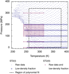
Figure 1: Location of the property data of the ST2(I) and ST2(II) models. The raw data obtained for both models are values of energy and density at each temperature and pressure point. For the ST2(II) model, the low-density fractions are also raw data. For the ST2(I) data, polynomials are fitted to the raw data for energy and density in the dashed region, to obtain values for the density on isobars and values for the response functions. Values for the low-density fraction on isobars are obtained by linear interpolation of the raw data.

The second version of the ST2 model has been investigated in Refs. Liu, Panagiotopoulos, and Debenedetti, 2009; Liu et al., 2012; Palmer, Car, and Debenedetti, 2013, and will be referred to as ST2(II). Data from the ST2(II) model were calculated from Monte Carlo simulations of 400 ST2 water molecules at constant pressure and temperature, with the Ewald treatment of electrostatics with vacuum boundary conditions. The raw data consist of density and energy as a function of temperature and pressure, at locations shown in Fig. 1. In addition, we computed the low-density fraction at each point, using the same criterion as for the ST2(I) model.

The approximations used in the formulation of the two-state thermodynamics, in particular Eq. (8), make our equation of state less accurate away from the critical point. This is why, to reduce the required number of background terms in Eq. (29), our equation of state was fitted to data in the reduced pressure ranges of 100 MPa to 250 MPa (ST2(I)) and 100 MPa to 300 MPa (ST2(II)). In the case of the ST2(I) data, the temperature range was also reduced to the range of 240 K to 322 K. For ST2(I), the equation of state was fitted to the volumes and response functions that were calculated from the polynomial fit, while for ST2(II), the equation was directly fitted to density and energy values obtained from simulations. The total number of the adjustable background coefficients is thus restricted to seven (see tables 1–4 in Appendix B). The parameter $c_{00}$ defines the zero point of energy. For the current ST2 simulations, the zero point of energy corresponds to moving all the molecules in the system infinitely far apart from one another.

III.2 Source of nonideality: energy-driven versus entropy-driven

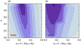
Figure 2: Contour lines of the sum of squared deviations $\chi^{2}$ of the data from the equation of state as a function of the effective interaction parameter $\omega$ given by Eq. (49) and $\delta$, the switching parameter between entropy-driven and energy-driven nonidealities, for the ST2(I) (a) and ST2(II) (b) models. Darker colors represent a better fit, where in (a), the darkest color represents $\chi^{2}\leq 2.5$, with subsequent contours corresponding to increases in $\chi^{2}$ by a factor of 1.6. In (b), the darkest color represents $\chi^{2}\leq 1.3$, and subsequent contours correspond to increases in $\chi^{2}$ by a factor of 1.3. For this analysis, the mean-field version of the equation of state is used, and the critical point location is fixed as 252 K, 165 MPa for ST2(I) and 247 K, 155 MPa for ST2(II).

Figure 2 shows the quality of the description of the ST2 data of versions I and II, with the nonideality factor $W$ given by Eq. (30), as a function of $\delta$ and the effective coefficient $\omega$,

$$\omega\equiv(1-\delta)\omega_{\text{a}}+\delta\omega_{\text{r}}.$$ (49)

For any value of $\delta$, a pressure dependence of $W$ appears to be necessary, with an optimum $\omega$ between 0.25 and 0.35. However, an energy-driven nonideality (with $\delta=1$) gives a much better result than entropy-driven nonideality (with $\delta=0$). Therefore, in subsequent sections, we adopt $\delta=1$.

III.3 Location of the liquid–liquid critical point

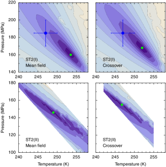
Figure 3: Location of the critical point for the mean-field equation (left) and the crossover equation (right), for the ST2(I) (top) and ST2(II) (bottom) models. Contours indicate the sum of squared deviations $\chi^{2}$ of the fit from the data, and darker colors represent lower deviations. For ST2(I), the darkest color represents $\chi^{2}\leq 4$, with subsequent contours corresponding to increases in $\chi^{2}$ by a factor of 1.6. For ST2(II), the darkest color represents $\chi^{2}\leq 0.4$, with subsequent contours corresponding to increases in $\chi^{2}$ by a factor of 1.6. The green dot shows the optimum critical point location. The blue dot with error bars represents the estimate by Cuthbertson and PooleCuthbertson and Poole (2011) of the location of the critical point.

Two approximations of the equation of state were considered: the mean-field equation described in Sec. II.2, and a renormalized equation of state that takes into account critical fluctuations and exhibits critical scaling behavior close to the critical point (Sec. II.3). The latter equation of state crosses over to mean-field behavior away from the critical point. Figure 3 shows how the goodness of the fit of both equations depends on the location of the critical point, for both the ST2(I) and ST2(II) model. For both ST2 models, the optimum critical point location for the crossover equation is at lower temperature and higher pressure than that of the mean-field equation. For the ST2(I) model, the location of the critical point predicted by the crossover equation is close to the estimate of Cuthbertson and Poole,Cuthbertson and Poole (2011) although outside of the reported error bars. Taking into account critical fluctuations causes a shift of the critical point in the direction of the two-phase region.Anisimov et al. (1992); Edison, Anisimov, and Sengers (1998); Povodyrev, Anisimov, and Sengers (1999) The shift in pressure is about 8 MPa, which is 7% of $\rho_{\text{c}}RT_{\text{c}}$.

The Gibbs energy of mixing $\Delta\hat{G}$, given by Eq. (31), is symmetric with respect to the order parameter $\phi_{1}=2x-1$. This means that in our equation of state the Widom line corresponds to the low-density fraction $x=1/2$ and to the inflection point in the fraction versus temperature. The low-density fraction was also found to be be $1/2$ at the Widom line in the simulated TIP4P/2005 model.Wikfeldt, Nilsson, and Pettersson (2011) However, in our equation of state this is a simplification, valid only close to the critical point. Figure 4 shows that for ST2(I), the locations of $x=1/2$ and the inflection points become different upon departure from the critical point, with our prediction being a compromise between these two. To improve this feature, one needs to introduce some asymmetry with respect to the low-density fraction $x$ in the Gibbs energy of mixing [Eq. (31)], and go beyond the linear approximation in the expression for $\ln K$ [Eq. (8)].

For the ST2(II) model, the shift in critical pressure between the mean-field and crossover critical point locations is about 9 MPa (Fig. 3). The optimum critical temperatures that we find (249.0 K for the mean-field equation and 246.8 K for the crossover equation) do not agree with the 2009 estimate of Liu et al. Liu, Panagiotopoulos, and Debenedetti (2009) of $237\pm 4$ K shown in Fig. 4. However, the liquid–liquid transition line that we find does agree with the points at 223 K and 228.6 K that Liu et al. Liu et al. (2012) estimated in 2012.

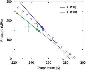
Figure 4: Comparison of critical point locations and liquid–liquid transition lines for the ST2(I) and ST2(II) models. Open circles (with error bars) are critical point locations reported in Refs Cuthbertson and Poole, 2011; Liu, Panagiotopoulos, and Debenedetti, 2009. Closed circles and squares: fitted location of critical point according to the mean-field or crossover equation, respectively. The lines are the liquid–liquid transition lines (solid) and Widom lines (dashed). Open diamonds are points with a low-density fraction equal to 1/2 (ST2(I)).Cuthbertson and Poole (2011) Triangles: inflection points in the low-density fraction versus temperature. Open squares: estimated locations of phase transitionLiu et al. (2012) (ST2(II))

III.4 Description of thermodynamic properties

Figure 5 shows thermodynamic-property data from the polynomial fit of the ST2(I) model, together with predictions from the equation of state. The predictions match the data well. In the region where ST2(I) data are available, the fits of the mean-field and crossover equations are almost indistinguishable. This is why the curves for the properties are shown only for the crossover equation, except for the liquid–liquid coexistence curve, for which the shapes are different in the close vicinity of the critical point. In Fig. 6, the raw ST2(I) data are shown in an energy–density plot. The molar energy $E$ is calculated as

$$E=G+TS-PV.$$ (50)

The equation of state agrees well with the data, except for three isotherms at low density and low temperatures.

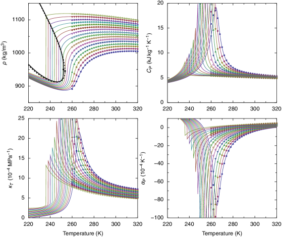
Figure 5: Density $\rho$, isobaric heat capacity $C_{P}$, isothermal compressibility $\kappa_{T}$, and expansivity $\alpha_{P}$ along isobars, predicted by the crossover equation of state. The data points are obtained from polynomial fits to raw data for the volume and energy for the ST2(I) model. In the density graph, the black curves indicate the phase coexistence densities (dashed: mean-field equation, solid: crossover equation), and the black dots represent the mean-field and crossover locations for the critical point. Isobar pressures are 100 MPa to 250 MPa in steps of 10 MPa.

Figure 6: Isotherms of energy $E$ versus density $\rho$, for the ST2(I) model (points) and predictions by the crossover equation of state. The black curves indicate phase coexistence (dashed: mean-field equation, solid: crossover equation), and the black dots represent the mean-field and crossover locations for the critical point. From bottom to top, the isotherm temperatures are 240 K to 320 K in steps of 5 K.

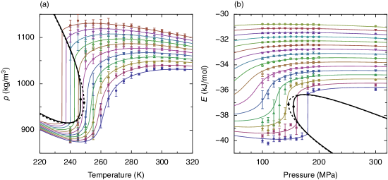
Figure 7: Density $\rho$ (a) and molar energy $E$ (b) obtained for the ST2(II) model (points) and predicted by the crossover equation of state. The black curves indicate two-phase coexistence (dashed: mean-field equation, solid: crossover equation), and the black dots represent the critical point. In (a) the isobar pressures are 100 MPa to 200 MPa in steps of 10 MPa. In (b), the isotherm temperatures are 240 K to 315 K in steps of 5 K.

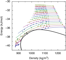
Figure 8: Isotherms of energy $E$ versus density $\rho$, for the ST2(II) model (points) and predictions by the crossover two-state equation. The black curves indicate phase coexistence (dashed: mean-field equation, solid: crossover equation), and the black dots represent the critical point. From bottom to top, the isotherm temperatures are 240 K to 315 K in steps of 5 K.

For the ST2(II) model, the equation of state was fitted to the raw data. The results are shown in Figs. 7 and 8. It is seen from both figures that the quality of the description of the density and energy is even better than for the ST2(I) model, in particular for low density and low temperature.

The numerical values of the parameters of the equation of state are given in tables 1–4.

III.5 Low-density fraction

The low-density fractions $x$ predicted (not fitted) by the equation of state are shown in Fig. 9. The fractions predicted by the mean-field equation and the crossover equation are indistinguishable, except for the fraction at the liquid–liquid coexistence in the close vicinity to the critical point. For both ST2 models, the predictions do qualitatively represent the low-density fraction. For ST2(I), where data are available close to the critical point, the predictions are quantitatively good.

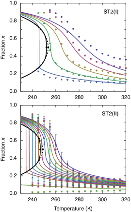
Figure 9: Low-density fraction from the ST2(I) and ST2(II) models (points) and the predictions from the crossover equation of state. The black curves indicate the phase coexistence fractions (dashed: mean-field equation, solid: crossover equation). For ST2(I), the isobar pressures are 0 MPa to 200 MPa in steps of 50 MPa. For ST2(II), the isobar pressures are 100 MPa to 200 MPa in steps of 10 MPa, followed by 300 MPa.

IV Discussion and conclusion

Figure 10: Heat capacity at constant volume $C_{V}$ along the critical isobar, $P=P_{\text{c}}$, predicted for the ST2(II) model for the mean-field equation (dashed) and crossover equation (solid).

Our analysis of the two versions of the ST2 model could not detect significant deviations from the mean-field approximation of the equation of state. To unambiguously detect the effects of the critical fluctuations, we would need more data close to the critical point. With the data currently available, the location of the critical point for both versions of the ST2 model is still not certain enough. Secondly, for the properties analyzed the effects of fluctuations are not very pronounced. There is one property whose anomaly solely originates from the fluctuation effects. This is the heat capacity at constant volume $C_{V}$ which weakly diverges at the critical point in scaling theory and remains finite in the mean-field approximation.Anisimov and Sengers (2000); Behnejad, Sengers, and Anisimov (2010) We have calculated $C_{V}$ as a function of temperature along the critical isobar. The result is shown in Fig. 10 for the ST2(II) model. In the crossover equation, the peak of $C_{V}$ is very narrow (within 0.1 K). This feature makes such a peak undetectable within the accuracy of the simulations, which have temperature increments of 5 K. For real supercooled water, it was also impossible to distinguish between the mean-field approximation and effects of the critical fluctuations, because of the lack of experimental data in the critical region. A parametric equation of state which obeys the asymptotic scaling laws was applied to describe the thermodynamic properties of supercooled water in Refs. Fuentevilla and Anisimov, 2006; Bertrand and Anisimov, 2011; Holten et al., 2012. The crossover to mean-field behavior away from the critical point was absorbed in the adjustable backgrounds. The quality of the description was similar to that of the two-state equation.Holten and Anisimov (2012a)

The order parameter in our equation of state, $\phi_{1}$, is introduced phenomenologically through the low-density fraction. We assume that the order parameter thermodynamically belongs to the same universality class as the order parameter near the vapor–liquid transition (associated with the density). However, because the low-density fraction relaxes through a reorientation of molecular bonds, dynamically, the order parameter may belong to the nonconserved-order-parameter universality class,Tanaka (1999); Biddle et al. (2013) even if this order parameter is coupled with conserved properties, density and energy, through Eqs. (23) and (24).

The results presented in previous sections show that the two-state physics reasonably describes the properties of both versions of the ST2 model of water. It is interesting to compare the application of this approach to two alternative models of water, ST2 and mW. While the nonideality in mixing of the two states in the mW model is not strong enough to cause a metastable liquid–liquid separation, the ST2 model does show the metastable liquid–liquid transition, terminated by a critical point. Phenomenologically, the reason for the different behavior of these two models may be associated with the source of the nonideality. As shown in Ref. Holten et al., 2013, in the mW model the nonideality is purely entropy-driven (athermal mixing of two structures), while in the ST2 model the nonideality is mainly energy-driven. As discussed in Ref. Holten et al., 2013, the physical origin of the excess entropy of mixing in the mW model can be attributed to the clustering of the molecules involved in the low-density structure. The clustering significantly suppresses the entropy of mixing. A similar effect is well known for mixtures of high-molecular-weight polymers, where the number of statistical configurations is restricted by polymerization.Flory (1953) However, this effect alone cannot cause phase separation without some contribution from the enthalpy of mixing, which is almost nonexistent in the mW model.Holten et al. (2013)

We remain agnostic with respect to the most intriguing question: whether real liquid water exhibits a metastable liquid–liquid transition or not. We do not, in other words, address the question of whether real liquid water is closer to mW or to ST2. It was shown in Ref. Holten and Anisimov, 2012a that the anomalies of supercooled water can be described by the nearly athermal, entropy-driven nonideality of mixing of the two states, similar to mW. However, is the magnitude of the nonideality sufficient to cause the metastable liquid–liquid separation? To answer this question, significantly more accurate experiments on the response functions, as well as independent measurements of the low-density fraction as a function of temperature and pressure in real water are desirable.

Appendix A Derivation of Eqs. (23)–(28)

Critical phenomena can be characterized by the scaling fields $h_{1}$ and $h_{2}$, which are given for our equation of state by Eqs. (13) and (14),

$$h_{1} =\ln K,$$ (51)

$$h_{2} =2-W,$$ (52)

and a dependent scaling field $h_{3}(h_{1},h_{2})$, which is the critical part of the field-dependent thermodynamic potential. For our equation of state, we adopt the formHolten and Anisimov (2012b)

$$h_{3}=-\frac{2(\hat{G}-\hat{G}^{\text{A}})}{\hat{T}}-\ln K+\frac{W}{2}.$$ (53)

The scaling fields are connected to the scaling densities $\phi_{1}$ and $\phi_{2}$ by the relation

$$\mathrm{d}h_{3}=\phi_{1}\mathrm{d}h_{1}+\phi_{2}\mathrm{d}h_{2},$$ (54)

so that

$$\phi_{1}=\left(\frac{\partial{h_{3}}}{\partial{h_{1}}}\right)_{h_{2}},\qquad\phi_{2}=\left(\frac{\partial{h_{3}}}{\partial{h_{2}}}\right)_{h_{1}}.$$ (55)

All thermodynamic properties can be written as derivatives of the dimensionless Gibbs energy $\hat{G}$. From Eq. (53) it follows that

$$\hat{G}=-\frac{\hat{T}}{2}\left(h_{3}+\ln K-\frac{W}{2}\right)+\hat{G}^{\text{A}}.$$ (56)

The dimensionless volume $\hat{V}$ can then be written as

$$\hat{V}=\left(\frac{\partial{\hat{G}}}{\partial{\hat{P}}}\right)_{\hat{T}}=-\frac{\hat{T}}{2}\left[\left(\frac{\partial{h_{3}}}{\partial{\hat{P}}}\right)_{\hat{T}}+a\lambda-\frac{W_{\hat{P}}}{2}\right]+\hat{G}^{\text{A}}_{\hat{P}}.$$ (57)

The pressure derivative of $h_{3}$ is found from Eq. (54),

$$\left(\frac{\partial{h_{3}}}{\partial{\hat{P}}}\right)_{\hat{T}} =\phi_{1}\left(\frac{\partial{h_{1}}}{\partial{\hat{P}}}\right)_{\hat{T}}+\phi_{2}\left(\frac{\partial{h_{2}}}{\partial{\hat{P}}}\right)_{\hat{T}}$$

$$=\phi_{1}a\lambda-\phi_{2}W_{\hat{P}}.$$ (58)

When we substitute this result in Eq. (57), we obtain Eq. (23). The dimensionless entropy $\hat{S}$ is related to the Gibbs energy as

$$\hat{S} =-\left(\frac{\partial{\hat{G}}}{\partial{\hat{T}}}\right)_{\hat{P}}$$

$$=\frac{\hat{T}}{2}\left[\left(\frac{\partial{h_{3}}}{\partial{\hat{T}}}\right)_{\hat{P}}+\lambda-\frac{W_{\hat{T}}}{2}\right]+\frac{1}{2}\left(h_{3}+\ln K-\frac{W}{2}\right)-\hat{G}^{\text{A}}_{\hat{T}}$$

$$=\frac{\hat{T}}{2}\left[\phi_{1}\lambda-\phi_{2}W_{\hat{T}}+\lambda-\frac{W_{\hat{T}}}{2}\right]-\frac{\hat{G}-\hat{G}^{\text{A}}}{\hat{T}}-\hat{G}^{\text{A}}_{\hat{T}},$$ (59)

where the temperature derivative of $h_{3}$ was obtained analogously to Eq. (58). This result for $\hat{S}$ leads to Eq. (24).

The dimensionless response functions are expressed in terms of the scaling susceptibilities $\chi_{1}$, $\chi_{12}$, and $\chi_{2}$, which are connected to the scaling densities by the relations

$$\mathrm{d}\phi_{1} =\chi_{1}\mathrm{d}h_{1}+\chi_{12}\mathrm{d}h_{2},$$ (60)

$$\mathrm{d}\phi_{2} =\chi_{12}\mathrm{d}h_{1}+\chi_{2}\mathrm{d}h_{2}.$$ (61)

The dimensionless compressibility $\hat{\kappa}_{T}$ is related to $\hat{V}$ as

$$\hat{\kappa}_{T}\hat{V}=-\left(\frac{\partial{\hat{V}}}{\partial{\hat{P}}}\right)_{\hat{T}}=\frac{\hat{T}}{2}\left[a\lambda\left(\frac{\partial{\phi_{1}}}{\partial{\hat{P}}}\right)_{\hat{T}}-W_{\hat{P}}\left(\frac{\partial{\phi_{2}}}{\partial{\hat{P}}}\right)_{\hat{T}}\right]-\hat{G}^{\text{A}}_{\hat{P}\hat{P}},$$ (62)

under the assumption that $W_{\hat{P}\hat{P}}=0$. The pressure derivative of $\phi_{1}$ is found from Eq. (60),

$$\left(\frac{\partial{\phi_{1}}}{\partial{\hat{P}}}\right)_{\hat{T}} =\chi_{1}\left(\frac{\partial{h_{1}}}{\partial{\hat{P}}}\right)_{\hat{T}}+\chi_{2}\left(\frac{\partial{h_{2}}}{\partial{\hat{P}}}\right)_{\hat{T}}$$

$$=\chi_{1}a\lambda+\chi_{12}W_{\hat{P}},$$ (63)

and the pressure derivative of $\phi_{2}$ is found analogously from Eq. (61).

The dimensionless expansivity $\hat{\alpha}_{P}$ and heat capacity $\hat{C}_{P}$ are found from the relations

$$\hat{\alpha}_{P}\hat{V}=\left(\frac{\partial{\hat{V}}}{\partial{\hat{T}}}\right)_{\hat{P}},\qquad\frac{\hat{C}_{P}}{\hat{T}}=\left(\frac{\partial{\hat{S}}}{\partial{\hat{T}}}\right)_{\hat{P}},$$ (64)

which are evaluated in the same manner as Eq. (62).

Appendix B Tables

For all fits, the parameter $c_{01}$ is given by

$$c_{01}=1+a\lambda/2-\omega_{\text{r}}/4,$$ (65)

to ensure that $\hat{V}=1$ at the critical point. The parameter $c_{00}$ defines the zero point of energy, as described in Sec. III.1. The parameter $c_{10}$ defines the zero point of entropy and was taken zero. The molecular cutoff parameter in the crossover procedure is optimized by trial at the value $\Lambda=0.3$ for both versions of the ST2 model.

Table 1: Parameters for the mean-field equation fitted to ST2(I)

Parameter	Value	Parameter	Value
$T_{\text{c}}$	$253.5~{}\text{K}$	$c_{02}$	$-7.275\;1\times 10^{-3}$
$P_{\text{c}}$	$160.0~{}\text{MPa}$	$c_{03}$	$-2.330\;2\times 10^{-3}$
$\rho_{\text{c}}$	$52.478~{}\text{kmol m^{-3}}$	$c_{11}$	$1.950\;3\times 10^{-1}$
$\lambda$	$-3.491\,5$	$c_{12}$	$-2.765\;1\times 10^{-2}$
$a$	$0.085\,811$	$c_{13}$	$1.202\;0\times 10^{-2}$
$\omega_{\text{r}}$	$0.231\,65$	$c_{20}$	$-5.830\;3$
$c_{00}$	$-1.664\;6\times 10^{1}$	$c_{30}$	$2.115\;0$

Table 2: Parameters for the crossover equation fitted to ST2(I)

$T_{\text{c}}$	$252.0~{}\text{K}$	$c_{02}$	$-8.350\;6\times 10^{-3}$
$P_{\text{c}}$	$168.0~{}\text{MPa}$	$c_{03}$	$-2.006\;6\times 10^{-3}$
$\rho_{\text{c}}$	$52.739~{}\text{kmol m^{-3}}$	$c_{11}$	$1.855\;0\times 10^{-1}$
$\lambda$	$-3.464\,3$	$c_{12}$	$-2.145\;7\times 10^{-2}$
$a$	$0.085\,496$	$c_{13}$	$1.078\;2\times 10^{-2}$
$\omega_{\text{r}}$	$0.238\,02$	$c_{20}$	$-5.856\;6$
$c_{00}$	$-1.677\;7\times 10^{1}$	$c_{30}$	$2.092\;5$

Table 3: Parameters for the mean-field equation fitted to ST2(II)

Parameter	Value	Parameter	Value
$T_{\text{c}}$	$249.0~{}\text{K}$	$c_{02}$	$-8.524\;1\times 10^{-3}$
$P_{\text{c}}$	$146.0~{}\text{MPa}$	$c_{03}$	$-1.323\;2\times 10^{-3}$
$\rho_{\text{c}}$	$53.261~{}\text{kmol m^{-3}}$	$c_{11}$	$2.405\;2\times 10^{-1}$
$\lambda$	$-3.202\,1$	$c_{12}$	$-1.199\;9\times 10^{-2}$
$a$	$0.119\,9$	$c_{13}$	$3.415\;1\times 10^{-3}$
$\omega_{\text{r}}$	$0.171\,81$	$c_{20}$	$-4.400\;7$
$c_{00}$	$-1.550\;9\times 10^{1}$	$c_{30}$	$1.768\;5$

Table 4: Parameters for the crossover equation fitted to ST2(II)

Parameter	Value	Parameter	Value
$T_{\text{c}}$	$246.75~{}\text{K}$	$c_{02}$	$-9.471\;7\times 10^{-3}$
$P_{\text{c}}$	$155.0~{}\text{MPa}$	$c_{03}$	$-1.099\;9\times 10^{-3}$
$\rho_{\text{c}}$	$53.645~{}\text{kmol m^{-3}}$	$c_{11}$	$2.340\;0\times 10^{-1}$
$\lambda$	$-3.179\,3$	$c_{12}$	$-8.685\;3\times 10^{-3}$
$a$	$0.120\,53$	$c_{13}$	$2.836\;9\times 10^{-3}$
$\omega_{\text{r}}$	$0.171\,81$	$c_{20}$	$-4.408\;8$
$c_{00}$	$-1.568\;5\times 10^{1}$	$c_{30}$	$1.714\;6$

References

- Angell, Shuppert, and Tucker (1973) C. A. Angell, J. Shuppert, and J. C. Tucker, J. Phys. Chem. 77, 3092 (1973).
- Angell, Oguni, and Sichina (1982) C. A. Angell, M. Oguni, and W. J. Sichina, J. Phys. Chem. 86, 998 (1982).
- Tombari, Ferrari, and Salvetti (1999) E. Tombari, C. Ferrari, and G. Salvetti, Chem. Phys. Lett. 300, 749 (1999).
- Archer and Carter (2000) D. G. Archer and R. W. Carter, J. Phys. Chem. B 104, 8563 (2000).
- Speedy and Angell (1976) R. J. Speedy and C. A. Angell, J. Chem. Phys. 65, 851 (1976).
- Kanno and Angell (1979) H. Kanno and C. A. Angell, J. Chem. Phys. 70, 4008 (1979).
- Mishima (2010a) O. Mishima, J. Chem. Phys. 133, 144503 (2010a).
- Hare and Sorensen (1987) D. E. Hare and C. M. Sorensen, J. Chem. Phys. 87, 4840 (1987).
- Kanno and Angell (1980) H. Kanno and C. A. Angell, J. Chem. Phys. 73, 1940 (1980).
- Ter Minassian, Pruzan, and Soulard (1981) L. Ter Minassian, P. Pruzan, and A. Soulard, J. Chem. Phys. 75, 3064 (1981).
- Poole et al. (1992) P. H. Poole, F. Sciortino, U. Essmann, and H. E. Stanley, Nature (London) 360, 324 (1992).
- Mishima and Stanley (1998a) O. Mishima and H. E. Stanley, Nature 396, 329 (1998a).
- Stanley et al. (2000) H. E. Stanley, S. V. Buldyrev, M. Canpolat, O. Mishima, M. R. Sadr-Lahijany, A. Scala, and F. W. Starr, Phys. Chem. Chem. Phys. 2, 1551 (2000).
- Stokely et al. (2010) K. Stokely, M. G. Mazza, H. E. Stanley, and G. Franzese, Proc. Natl. Acad. Sci. U.S.A. 107, 1301 (2010).
- Tanaka (2000) H. Tanaka, Europhys. Lett. 50, 340 (2000).
- Mishima (2010b) O. Mishima, Proc. Jpn. Acad., Ser. B 86, 165 (2010b).
- Mishima and Stanley (1998b) O. Mishima and H. E. Stanley, Nature 392, 164 (1998b).
- Mishima (2000) O. Mishima, Phys. Rev. Lett. 85, 334 (2000).
- Mishima (2011) O. Mishima, J. Phys. Chem. B 115, 14064 (2011).
- Amann-Winkel et al. (2013) K. Amann-Winkel, C. Gainaru, P. H. Handle, M. Seidl, H. Nelson, R. Böhmer, and T. Loerting, Proc. Natl. Acad. Sci. U.S.A. 110, 17720 (2013).
- General Discussion (2013) General Discussion, Faraday Discuss. 167, 109 (2013).
- Stillinger and Rahman (1974) F. H. Stillinger and A. Rahman, J. Chem. Phys. 60, 1545 (1974).
- Liu, Panagiotopoulos, and Debenedetti (2009) Y. Liu, A. Z. Panagiotopoulos, and P. G. Debenedetti, J. Chem. Phys. 131, 104508 (2009).
- Sciortino, Saika-Voivod, and Poole (2011) F. Sciortino, I. Saika-Voivod, and P. H. Poole, Phys. Chem. Chem. Phys. 13, 19759 (2011).
- Liu et al. (2012) Y. Liu, J. C. Palmer, A. Z. Panagiotopoulos, and P. G. Debenedetti, J. Chem. Phys. 137, 214505 (2012).
- Kesselring et al. (2012) T. A. Kesselring, G. Franzese, S. V. Buldyrev, H. J. Herrmann, and H. E. Stanley, Sci. Rep. 2, 474 (2012).
- Kesselring et al. (2013) T. A. Kesselring, E. Lascaris, G. Franzese, S. V. Buldyrev, H. J. Herrmann, and H. E. Stanley, J. Chem. Phys. 138, 244506 (2013).
- Cuthbertson and Poole (2011) M. J. Cuthbertson and P. H. Poole, Phys. Rev. Lett. 106, 115706 (2011).
- Poole et al. (2013) P. H. Poole, R. K. Bowles, I. Saika-Voivod, and F. Sciortino, J. Chem. Phys. 138, 034505 (2013).
- Palmer, Car, and Debenedetti (2013) J. C. Palmer, R. Car, and P. G. Debenedetti, Faraday Discuss. 167, 77 (2013).
- Steinhardt, Nelson, and Ronchetti (1983) P. J. Steinhardt, D. R. Nelson, and M. Ronchetti, Phys. Rev. B 28, 784 (1983).
- Limmer and Chandler (2011) D. T. Limmer and D. Chandler, J. Chem. Phys. 135, 134503 (2011).
- Limmer and Chandler (2013) D. T. Limmer and D. Chandler, J. Chem. Phys. 138, 214504 (2013).
- English, Kusalik, and Tse (2013) N. J. English, P. G. Kusalik, and J. S. Tse, J. Chem. Phys. 139, 084508 (2013).
- Molinero and Moore (2009) V. Molinero and E. B. Moore, J. Phys. Chem. B 113, 4008 (2009).
- Moore and Molinero (2011) E. B. Moore and V. Molinero, Nature 479, 506 (2011).
- Moore and Molinero (2009) E. B. Moore and V. Molinero, J. Chem. Phys. 130, 244505 (2009).
- Nilsson, Huang, and Pettersson (2012) A. Nilsson, C. Huang, and L. G. Pettersson, J. Mol. Liq. 176, 2 (2012).
- Taschin et al. (2013) A. Taschin, P. Bartolini, R. Eramo, R. Righini, and R. Torre, Nat. Commun. 4, 2401 (2013).
- Wikfeldt, Nilsson, and Pettersson (2011) K. T. Wikfeldt, A. Nilsson, and L. G. M. Pettersson, Phys. Chem. Chem. Phys. 13, 19918 (2011).
- Holten and Anisimov (2012a) V. Holten and M. A. Anisimov, Sci. Rep. 2, 713 (2012a).
- Tokushima et al. (2008) T. Tokushima, Y. Harada, O. Takahashi, Y. Senba, H. Ohashi, L. G. M. Pettersson, A. Nilsson, and S. Shin, Chem. Phys. Lett. 460, 387 (2008).
- Wernet et al. (2004) Ph. Wernet, D. Nordlund, U. Bergmann, M. Cavalleri, M. Odelius, H. Ogasawara, L. Å. Näslund, T. K. Hirsch, L. Ojamäe, P. Glatzel, L. G. M. Pettersson, and A. Nilsson, Science 304, 995 (2004).
- Huang et al. (2009) C. Huang, K. T. Wikfeldt, T. Tokushima, D. Nordlund, Y. Harada, U. Bergmann, M. Niebuhr, T. M. Weiss, Y. Horikawa, M. Leetmaa, M. P. Ljungberg, O. Takahashi, A. Lenz, L. Ojamäe, A. P. Lyubartsev, S. Shin, L. G. M. Pettersson, and A. Nilsson, Proc. Natl. Acad. Sci. U.S.A. 106, 15214 (2009).
- Xu et al. (2009) L. Xu, F. Mallamace, Z. Yan, F. W. Starr, S. V. Buldyrev, and H. E. Stanley, Nature Phys. 5, 565 (2009).
- Holten et al. (2013) V. Holten, D. T. Limmer, V. Molinero, and M. A. Anisimov, J. Chem. Phys. 138, 174501 (2013).
- Bertrand and Anisimov (2011) C. E. Bertrand and M. A. Anisimov, J. Phys. Chem. B 115, 14099 (2011).
- Tanaka (2013) H. Tanaka, Faraday Discuss. 167, 9 (2013).
- Tu et al. (2012) Y. Tu, S. V. Buldyrev, Z. Liu, H. Fang, and H. E. Stanley, EPL 97, 56005 (2012).
- Xu et al. (2006) L. Xu, S. V. Buldyrev, C. A. Angell, and H. E. Stanley, Phys. Rev. E 74, 031108 (2006).
- Whiting (1884) H. Whiting, Proc. Am. Acad. Arts Sci. 19, 353 (1884).
- Röntgen (1892) W. C. Röntgen, Ann. Phys. (Leipzig) 281, 91 (1892).
- McMillan (2004) P. F. McMillan, J. Mater. Chem. 14, 1506 (2004).
- Wilding, Wilson, and McMillan (2006) M. C. Wilding, M. Wilson, and P. F. McMillan, Chem. Soc. Rev. 35, 964 (2006).
- Vedamuthu, Singh, and Robinson (1994) M. Vedamuthu, S. Singh, and G. W. Robinson, J. Phys. Chem. 98, 2222 (1994).
- Ponyatovsky, Sinitsyn, and Pozdnyakova (1998) E. G. Ponyatovsky, V. V. Sinitsyn, and T. A. Pozdnyakova, J. Chem. Phys. 109, 2413 (1998).
- Moynihan (1996) C. T. Moynihan, Mat. Res. Soc. Symp. Proc. 455, 411 (1996).
- Prigogine and Defay (1954) I. Prigogine and R. Defay, Chemical Thermodynamics (Longmans, Green & Co., London, 1954).
- Xu et al. (2005) L. Xu, P. Kumar, S. V. Buldyrev, S.-H. Chen, P. H. Poole, F. Sciortino, and H. E. Stanley, Proc. Natl. Acad. Sci. U.S.A. 102, 16558 (2005).
- Fuentevilla and Anisimov (2006) D. A. Fuentevilla and M. A. Anisimov, Phys. Rev. Lett. 97, 195702 (2006), erratum ibid. 98, 149904 (2007).
- Holten et al. (2012) V. Holten, C. E. Bertrand, M. A. Anisimov, and J. V. Sengers, J. Chem. Phys. 136, 094507 (2012).
- Fisher (1983) M. E. Fisher, in Critical Phenomena, Lecture Notes in Physics, Vol. 186, edited by F. J. W. Hahne (Springer, Berlin, 1983) pp. 1–139.
- Anisimov and Sengers (2000) M. A. Anisimov and J. V. Sengers, in Equations of State for Fluids and Fluid Mixtures, Experimental Thermodynamics, Vol. V, edited by J. V. Sengers, R. F. Kayser, C. J. Peters, and H. J. White, Jr. (Elsevier, Amsterdam, 2000) Chap. 11, pp. 381–434.
- Behnejad, Sengers, and Anisimov (2010) H. Behnejad, J. V. Sengers, and M. A. Anisimov, in Applied Thermodynamics of Fluids, edited by A. R. H. Goodwin, J. V. Sengers, and C. J. Peters (RSC Publishing, Cambridge, UK, 2010) Chap. 10, pp. 321–367.
- Anisimov et al. (1992) M. A. Anisimov, S. B. Kiselev, J. V. Sengers, and S. Tang, Physica A 188, 487 (1992).
- Kim et al. (2003) Y. C. Kim, M. A. Anisimov, J. V. Sengers, and E. Luijten, J. Stat. Phys. 110, 591 (2003).
- Holten and Anisimov (2012b) V. Holten and M. A. Anisimov, Sci. Rep. 2, 713 (2012b), supplementary information.
- Edison, Anisimov, and Sengers (1998) T. A. Edison, M. A. Anisimov, and J. V. Sengers, Fluid Phase Equilib. 150–151, 429 (1998).
- van ’t Hof, Japas, and Peters (2001) A. van ’t Hof, M. L. Japas, and C. J. Peters, Fluid Phase Equilib. 192, 27 (2001).
- Pelissetto and Vicari (2002) A. Pelissetto and E. Vicari, Phys. Rep. 368, 549 (2002).
- Sengers and Shanks (2009) J. V. Sengers and J. G. Shanks, J. Stat. Phys. 137, 857 (2009).
- Povodyrev, Anisimov, and Sengers (1999) A. A. Povodyrev, M. A. Anisimov, and J. V. Sengers, Physica A 264, 345 (1999).
- Poole, Saika-Voivod, and Sciortino (2005) P. H. Poole, I. Saika-Voivod, and F. Sciortino, J. Phys.: Condens. Matter 17, L431 (2005).
- Tanaka (1999) H. Tanaka, J. Phys.: Condens. Matter 11, L159 (1999).
- Biddle et al. (2013) J. W. Biddle, V. Holten, J. V. Sengers, and M. A. Anisimov, Phys. Rev. E 87, 042302 (2013).
- Flory (1953) P. J. Flory, Principles of Polymer Chemistry (Cornell University Press, Ithaca, NY, 1953).