Structure of cylindrical electric double layers: Comparison of density functional and modified Poisson-Boltzmann theories with Monte Carlo simulations

Abstract

The structure of cylindrical double layers is studied using a modified Poisson Boltzmann theory and the density functional approach. In the model double layer, the electrode is a cylindrical polyion that is infinitely long, impenetrable, and uniformly charged. The polyion is immersed in a sea of equi-sized rigid ions embedded in a dielectric continuum. An in-depth comparison of the theoretically predicted zeta potentials, the mean electrostatic potentials, and the electrode-ion singlet density distributions is made with the corresponding Monte Carlo simulation data. The theories are seen to be consistent in their predictions that include variations in ionic diameters, electrolyte concentrations, and electrode surface charge densities, and are also capable of well reproducing some new and existing Monte Carlo results.

Key words: electric double layer, restricted primitive model, density profiles

PACS: 82.45.Fk, 61.20.Qg, 82.45.Gj

Abstract

Вивчено структуру цилiндричних подвiйних шарiв, використовуючи модифiковану теорiю Пуассона-Больцмана i теорiю функцiоналу густини. У цiй моделi подвiйного шару електродом є нескiнченно довгий, непроникний та однорiдно заряджений цилiндричний полiiон. Вiн оточений системою iонiв однакового розмiру у дiелектричному середовищi. Виконано докладне порiвняння результатiв теорiї для дзета потенцiалiв, для середнього електростатичного потенцiалу та для розподiлiв густини iон-електрод з даними комп’ютерного моделювання Монте Карло. Теоретичнi результати узгоджуються з новими та попереднiми даними моделювання Монте Карло при змiнi рiзних параметрiв, таких як iоннi дiаметри, концентрацiя електрода, густина заряду електрода.

Ключовi слова: подвiйний електричний шар, обмежена примiтивна модель, профiлi густини

1 Introduction

Description of the interactions and correlations of large polyions with the small, more mobile ions in the surrounding ionic cloud is of significance in situations ranging from fundamental life processes such as the transport of ions, water, and various molecules across cell membranes, flocculation in colloidal systems [1], industrial polyelectrolytes [2], and the native structure of DNA and various proteins [3, 4, 5]. The structure and thermodynamics of all these systems manifest the complex behaviour of small ions within the atmosphere. A detailed understanding of the static structural features is therefore central to assessing the relative effect of various control parameters in such phenomena.

The electrode (polyion) along with the neighbouring inhomogeneous ion layer constitute the electric double layer with the shape of the polyion determining the geometry of the double layer. Over the past few decades the planar double layer (PDL) has become synonymous with the electric double layer as it has been the one to have been extensively investigated through theoretical approaches, numerical simulation methods, and experimental techniques (see for example, references [6, 7] for recent reviews). This notwithstanding, other double layer systems, viz., the cylindrical double layer (CDL), the spherical double layer (SDL), and ellipsoidal double layer (ESDL) have been coming under increasing scrutiny in recent years.

A number of experimental techniques including the small angle x-ray and neutron scattering [8, 9], the optical imaging, and electrophoretic mobility measurements have been used to probe the properties of electric double layers [10, 11]. Recent advances in theoretical approaches and simulation methodologies have aided in the explanation of some of these experimental observations [12]. In most of the theoretical studies, the polyion is generally modelled as an infinitely long, hard, uniformly charged cylinder with the small ions being treated as charged hard spheres moving in a dielectric continuum. This is the so-called primitive model of the CDL. Of the theoretical studies mention ought to be made of the counterion condensation (CC) theory [13], the classical Poisson-Boltzmann (PB) description [14, 15], and the formal statistical mechanical approaches, for example, the integral equation theories [16, 17], the modified Poisson-Boltzmann theory (MPB) [18, 19, 20], and the density functional theory (DFT) [21, 22]. Parallel Monte Carlo (MC) simulations in various forms [23, 24, 25, 26, 27, 28, 9, 29, 30, 31, 32] have provided exact quantitative data for many model systems with regard to their structure and thermodynamics. However, many of these simulations have involved the cylindrical cell model [27, 28, 9, 29, 30, 31, 32] where the polyion is at a finite, non-zero concentration. By contrast, in the case of the CDL — our focus in this paper, the polyion is at infinite dilution, and in this situation the early MC simulations [23, 24, 25, 26] were somewhat limited in their scope. Indeed, in an earlier paper [33] two of us tried to compare the DFT and the MPB structural results for the primitive model CDL but the lack of detailed simulation data proved a hindrance and precluded a detailed comparison. The picture has now changed, however, with the availability of a new generation of MC simulation results due to Goel et al. [34]. This will permit a critical evaluation of these theories relative to the benchmark of the simulation data.

The DFT and MPB approaches to the electric double layer theory have come to be recognized as being two of the more successful ones for the planar [35], spherical [36, 37], and cylindrical [33] symmetries. In the PDL, in particular, both the theories have proved useful in describing the capacitance behaviour including capacitance anomaly at low temperatures [38]. The DFT techniques have evolved over the years since the initial applications to the PDL in the early 1990’s [39, 40, 41]. In recent years, a number of new formulations of DFT, coupled with different statistical mechanical approaches, have emerged as robust methods to study the systems involving correlations like the electric double layer [42]. A partially perturbative DFT procedure [21, 43] is adopted in the present work where the hard sphere part is determined through the weighted density approach (WDA) of Denton and Ashcroft [44], while the electrical contribution is a perturbation on the corresponding bulk electrolyte. The essential idea of the MPB theory is to incorporate within a potential formulation, the important missing elements in the classical PB formulation, namely, the inter-ionic correlations and the ionic exclusion volume effects. For the CDL, an MPB equation was first obtained by Outhwaite [18]. Numerical solutions were later developed by Bhuiyan and Outhwaite [19, 20] with some limited comparison with the hypernetted chain/mean spherical approximation [45, 46].

The first detailed comparative study of the DFT and the MPB structural results relative to MC simulations was undertaken by Bhuiyan and Outhwaite [35] for the PDL. The two theories were seen to be remarkably consistent over a wide range of physical parameters probed through the simulations [47]. A similar consistency between the theories was later observed by the same authors [36] with regard to structure in a SDL. An interesting result of the latter work is the charge inversion phenomenon observed in the MC simulations [48] for higher valencies, which was also reproduced by both the theories to a very good accuracy. It is thus natural to wonder if such trends will carry over to cylindrical symmetries.

In this paper we will explore the DFT and MPB theories for a primitive model CDL with a particular emphasis on the comparative behaviour of zeta potentials, density and mean electrostatic profiles vis-a-vis the Monte Carlo data. The zeta potentials are useful indicators of the capacitance characteristics of double layers and such comparison of these two theories in this regard has not appeared in the literature. Although our focus will be on DFT and MPB calculations at different physical states, we also intend to do MC simulations for new states.

2 Model and methods

As indicated in the previous section, in the model double layer system treated here, the polyion is mimicked by an infinitely long, non-polarizable, hard cylinder with a uniform surface charge density. The polyion is bathed by a restricted primitive model (RPM) electrolyte (equi-sized charged hard spheres moving in a dielectric continuum). The polyion surface charge density $\sigma$ is related to the axial charge $\xi$ through

$$\sigma=\frac{e}{2\pi Rb}=\frac{2\epsilon_{0}\epsilon_{\textrm{r}}}{\beta eR}\xi\,,$$ (1)

where $e$ is the fundamental charge, $b$ is the monomer length (length per unit charge), $\beta=(k_{\textrm{B}}T)^{-1}$, $k_{\textrm{B}}$ being the Boltzmann’s constant, and $T$ the temperature. The continuum solvent is characterized by the relative permittivity $\epsilon_{\textrm{r}}$ ($\epsilon_{0}$ is the vacuum permittivity), which is taken to be $\epsilon_{\textrm{r}}=78.358$, and $R$ is the radius of the polyion taken as $R=8\times 10^{-10}$ m. Following the previous work of Patra and Bhuiyan [33] we have set $T=298.15$ K, $b=1.7\times 10^{-10}$ m, and in most cases $\xi=4.2$ ($\sigma=0.187$ C/m²), which are the accepted values for a double-stranded DNA [26]. The other variable physical quantities will be described in the Results section. Denoting the charge of a small ion of species ${i}$ by $q_{i}=Z_{i}e$, with $Z_{i}$ being the ionic valency, the ion-ion interaction potential in the Hamiltonian can be written as

$$u_{ij}(r)=\left\{\begin{array}[]{ll}\infty,&\hbox{$r<a$},\\[4.30554pt] \displaystyle\frac{q_{i}q_{j}}{4\pi\epsilon_{0}\epsilon_{\textrm{r}}r},&\hbox{$r>a$,}\end{array}\right.$$ (2)

where $r$ is the distance between a pair of ions and $a$ is the common diameter of the ions of the bathing electrolyte. The bare interaction between an ion of species $i$ and the polyion is given by

$$u_{i}(r_{i})=v_{i}(r_{i})+w_{i}(r_{i}),$$ (3)

where $v_{i}(r_{i})$ and $w_{i}(r_{i})$ are the non-electrostatic and electrostatic (Coulombic) parts of the ion-polyion potential with $r_{i}$ being radial distance of ion $i$ from the polyion axis. The non-electrostatic contribution is a hard-core potential

$$v_{i}(r_{i})=\left\{\begin{array}[]{ll}\infty,&\hbox{$r_{i}<R+a/2$},\\ 0,&\hbox{$r_{i}>R+a/2$}.\end{array}\right.$$ (4)

The electrostatic part $w_{i}(r)$ is given by

$$w_{i}(r)=\left\{\begin{array}[]{ll}\displaystyle-\frac{eq_{i}}{2\pi\epsilon_{0}\epsilon_{\textrm{r}}b}{\ln}(r_{i}),&\hbox{$r_{i}\geqslant R+a/2$},\\ \infty,&\hbox{otherwise}.\end{array}\right.$$ (5)

The above double layer model was solved using the DFT and MPB techniques. The development of these theories has been chronicled elsewhere in the literature and will not be repeated here. For a summary of the principal equations that are used in the present calculations we refer the reader again to the earlier work by Patra and Bhuiyan [33]. The MC simulations were done in the canonical ensemble using the standard Metropolis algorithm and have been described by Goel et al. [34].

3 Results and discussion

     

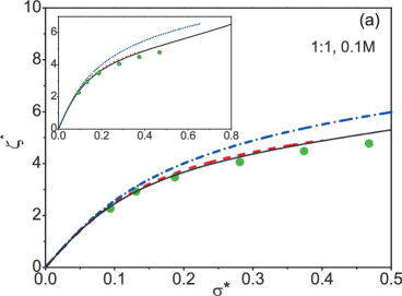
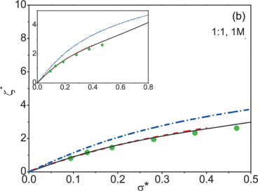
Figure 1: (Color online) Reduced zeta potential $\zeta^{*}$ [$=\psi^{*}(R/a+1/2)$] versus reduced surface charge density $\sigma^{*}$ for a 1:1 electrolyte at solution concentration (in mol/dm³ units) 0.1 M (panel a), 1 M (panel b), and 2 M (panel c) in a RPM cylindrical double layer. The symbols represent MC data, while the solid line represents the MPB results, the dashed line represents the DFT results, and the dash-dotted line shows the PB results. The polyion radius is $R=8\times 10^{-10}$ m, and the ionic diameter $a=4\times 10^{-10}$ m. MC data from reference [34].

     

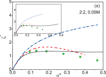
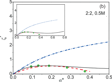
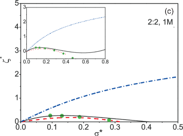
Figure 2: (Color online) Reduced zeta potential $\zeta^{*}$ [$=\psi^{*}(R/a+1/2)$] versus reduced surface charge density $\sigma^{*}$ for a 2:2 electrolyte at solution concentration (in mol/dm³ units) 0.05 M (panel a), 0.5 M (panel b), and 1 M (panel c) in a RPM cylindrical double layer. The symbols represent MC data, while the solid line represents the MPB results, the dashed line represents the DFT results, and the dash-dotted line shows the PB results. The polyion radius is $8\times 10^{-10}$ m, and the ionic diameter $a=4\times 10^{-10}$ m. MC data from reference [34].

     

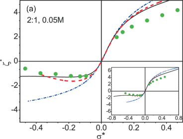
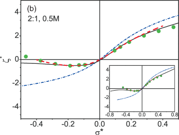
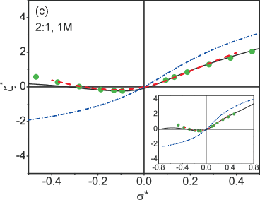
Figure 3: (Color online) Reduced zeta potential $\zeta^{*}$ [$=\psi^{*}(R/a+1/2)$] versus reduced surface charge density $\sigma^{*}$ for a 2:1/1:2 electrolyte at solution concentration (in mol/dm³ units) 0.05 M (panel a), 0.5 M (panel b), and 1 M (panel c) in a RPM cylindrical double layer. The symbols represent MC data, while the solid line represents the MPB results, the dashed line represents the DFT results, and the dash-dotted line shows the PB results. The polyion radius is $8\times 10^{-10}$ m, and the ionic diameter $a=4\times 10^{-10}$ m. MC data from reference [34].

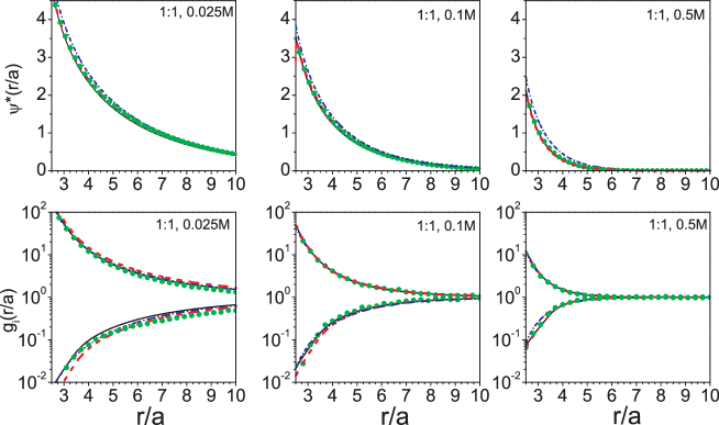
Figure 4: (Color online) Polyion-ion singlet distributions (lower panel) and the reduced mean electrostatic potentials (upper panel) for a 1:1 electrolyte surrounding a polyion with an axial charge parameter $\xi=4.2$ ($\sigma=0.187$ C/m²) and radius $R=8\times 10^{-10}$ m. The electrolyte concentrations are, from left to right, 0.025 M, 0.1 M, and 0.5 M, respectively. The rest of symbols and notation as in figure 1. The ionic diameter $a=4\times 10^{-10}$ m. MC data from reference [34].

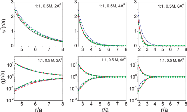
Figure 5: (Color online) Polyion-ion singlet distributions (lower panel) and the reduced mean electrostatic potentials (upper panel) for a 0.5 M 1:1 electrolyte surrounding a polyion with an axial charge parameter $\xi=4.2$ ($\sigma=0.187$ C/m²) and radius $R=8\times 10^{-10}$ m. The ionic diameters are, from left to right, 2, 4, and $6\times 10^{-10}$ m (in the labels Å $=10^{-10}$ m), respectively. The rest of symbols and notation as in figure 1. MC data from reference [34].

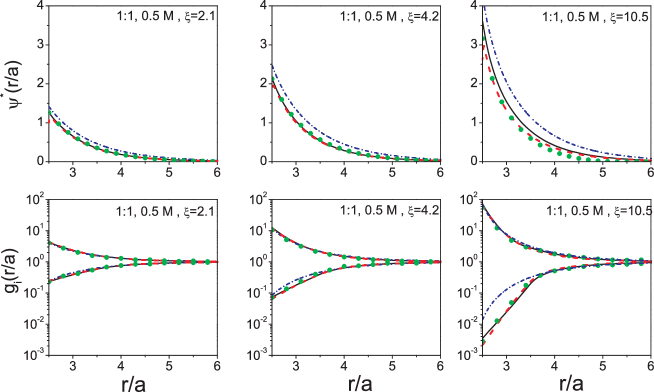
Figure 6: (Color online) Polyion-ion singlet distributions (lower panel) and the reduced mean electrostatic potentials (upper panel) for a 0.5 M 1:1 electrolyte surrounding a polyion with a radius $R=8\times 10^{-10}$ m. The polyion axial charge parameter $\xi$ values are, from left to right, 2.1 ($\sigma=0.0935$ C/m²), 4.2 ($\sigma=0.187$ C/m²), and 10.5 ($\sigma=0.468$ C/m²), respectively. The ionic diameter is $4\times 10^{-10}$ m The rest of symbols and notation as in figure 1. MC data from reference [34].

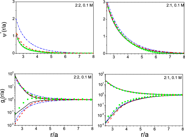
Figure 7: (Color online) Polyion-ion singlet distributions (lower panel) and the reduced mean electrostatic potentials (upper panel) for 2:2 and 2:1 electrolytes surrounding a polyion with an axial charge parameter $\xi=4.2$ ($\sigma=0.187$ C/m²) and radius $R=8\times 10^{-10}$ m. The electrolyte concentration is 0.1 M in each case. The rest of symbols and notation as in figure 1. The ionic diameter $a=4\times 10^{-10}$ m.

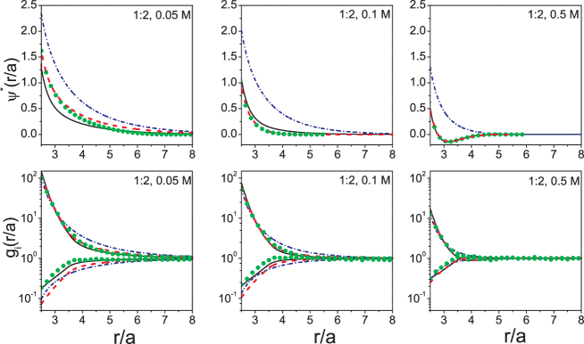
Figure 8: (Color online) Polyion-ion singlet distributions (lower panel) and the reduced mean electrostatic potentials (upper panel) for a 1:2 electrolyte surrounding a polyion with an axial charge parameter $\xi=4.2$ ($\sigma=0.187$ C/m²) and radius $R=8\times 10^{-10}$ m. The electrolyte concentrations are, from left to right, 0.05 M, 0.1 M, and 0.5 M, respectively. The rest of symbols and notation as in figure 1. The ionic diameter $a=4\times 10^{-10}$ m. MC data from reference [34].

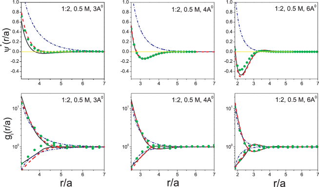
Figure 9: (Color online) Polyion-ion singlet distributions (lower panel) and the reduced mean electrostatic potentials (upper panels) for a 0.5 M 1:2 electrolyte surrounding a polyion with an axial charge parameter $\xi=4.2$ ($\sigma=0.187$ C/m²) and radius $R=8\times 10^{-10}$ m. The ionic diameters are, from left to right, 3, 4, and $6\times 10^{-10}$ m (in the labels Å $=10^{-10}$ m), respectively. The rest of symbols and notation as in figure 1. MC data from reference [34].

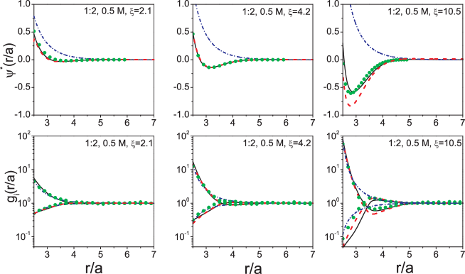
Figure 10: (Color online) Polyion-ion singlet distributions (lower panel) and the reduced mean electrostatic potentials (upper panel) for a 0.5 M 1:2 electrolyte surrounding a polyion with a radius $R=8\times 10^{-10}$ m. The polyion axial charge parameter $\xi$ values are, from left to right, 2.1 ($\sigma=0.0935$ C/m²), 4.2 ($\sigma=0.187$ C/m²), and 10.5 ($\sigma=0.468$ C/m²), respectively. The ionic diameter is $4\times 10^{-10}$ m The rest of symbols and notation as in figure 1. MC data from reference [34].

The DFT and MPB equations were solved numerically following the procedure given in references [39, 43] for DFT and [49, 50, 51] for MPB. During the course of calculations we generally considered the following ranges of variation for some of the physical parameters: the electrolyte concentration $c$ from 0.05 mol/dm³ to 2 mol/dm³, the ionic diameter $a$ from $2\times 10^{-10}$ m to $6\times 10^{-10}$ m, and the axial charge factor $\xi$ from 2.1 ($\sigma=0.0935$ C/m²) to 10.5 ($\sigma=0.468$ C/m²). These parameters were chosen to be in line with the existing MC data [34]. It ought to be mentioned though that the same ranges of variation for the same parameters were not strictly maintained for all the electrolyte systems treated. For comparison purposes we have also obtained numerical solution of the classical PB theory at the same set of physical states. In describing the results we will use universal reduced parameters for convenience, the relevant ones in the present case being $\sigma^{\ast}(=\sigma d^{2}/e)$ for the reduced surface charge density, and $\psi^{\ast}(r)$ [$=\beta e\psi(r)$] for the reduced mean electrostatic potential.

3.1 Zeta potential

We begin this discussion by considering the zeta potential profile as a function of polyion surface charge density $\sigma$, salt concentration $c$, and ionic valency $Z_{i}$. The zeta potential is defined in the polyelectrolyte literature as the mean electrostatic potential at the closest approach between the small ion and the charged polyion, that is, $\zeta=\psi(R+a/2)$. Figures 1–3 depict the reduced zeta potential profiles $\zeta^{*}=\psi^{*}(R/a+1/2)$ with respect to the reduced surface charge density $\sigma^{*}$. In these calculations, the ionic diameter is held fixed at $a=4\times 10^{-10}$ m. The results for a 1:1 electrolyte system at three different electrolyte concentrations $c=0.1$ mol/dm³, 1 mol/dm³, and 2 mol/dm³ are shown in figures 1 (a)–(c). In all cases the MC $\zeta^{*}$ is monotonic and increases continuously with $\sigma^{*}$, although the rate of increment decreases at the higher salt concentration. The PB results overestimate the MC $\zeta^{*}$ for the same $\sigma^{*}$ and this deviation increases with concentration. This is of course a well known feature of the mean field result in that the theory is more useful for monovalent systems at low concentrations where the effect of the neglected inter-ionic correlations is relatively less. One of the more noteworthy features of figure 1 is the quantitative agreement of the DFT and MPB predictions with MC results at all concentrations and over the whole range of $\sigma^{*}$ studied. A similar level of agreement between the two approaches was seen for the PDL [35] and the SDL [36].

As we move on to 2:2 systems in figure 2, the striking feature is that the MC, DFT, and MPB $\zeta^{*}$ are no longer monotonic. Indeed, the MC $\zeta^{*}$ shows a maximum before starting to decrease at high $\sigma^{*}$. Both DFT and MPB $\zeta^{*}$ follow the MC trends closely. At still higher surface charges, viz., $\sigma^{*}\gtrsim 0.5$, the MPB shows a shallow valley before increasing again as can be seen in the insets. This trend is probably an artefact of the theory. The PB results are monotonic and are thus not even qualitative with the simulations.

Figure 3 shows the $\zeta^{*}$ for an asymmetric 2:1/1:2 valency electrolyte. In the region $\sigma^{*}>$ 0 we have univalent counterions, while in the region $\sigma^{*}<$ 0 the counterions are divalent. It is interesting to observe that the characteristics of the zeta potential for the 2:1 and 1:2 systems resemble that for 1:1 in figure 1, and 2:2 in figure 2, respectively. This is clearly indicative of the well known result that it is the electrode-counterion interaction that governs double layer properties. Although not clearly visible at the scale of the figures, the MC, DFT, and MPB reveal a non-zero potential of zero charge (pzc), which is a consequence of asymmetry in the system. Besides, both DFT and MPB show good overall agreements with the simulations. The PB theory, however, does not reveal any non-zero pzc and is again not qualitative with the MC results for 1:2 systems. We remark further that the maxima or minima in $\zeta^{*}$ have been predicted previously theoretically and through simulations for the PDL [35, 47, 52, 53] and the SDL [54, 36, 37, 55, 56], and have also been observed earlier for the CDL [19, 20, 45, 46].

3.2 Double layer structure

3.2.1 1:1 electrolytes

We now focus on the static structural properties of the CDL given in figures 4–10. In the three figures 4, 5, and 6 we will compare the theoretical results with the available MC data [34] for ionic density distributions as well as the mean electrostatic potentials for 1:1 salts at different parametric conditions. Figure 4 depicts variation in concentration of the salt while keeping all other parameters fixed, and in particular, $a=4\times 10^{-10}$ m and $\xi=4.2$ ($\sigma=0.187$ C/m²). As might be expected, there is an excessive accumulation of counterions near the polyion surface, which continuously decays down to the bulk. All the $\psi^{*}(r)$ and $g_{i}(r)$ are monotonically decreasing with the DFT and MPB results being virtually indistinguishable from the MC results. With an increase in electrolyte concentration, this decrease becomes more rapid and the double layer becomes progressively less diffuse. An increase of concentration also leads to an increase in coion contact value and to a decrease in counterion contact value. This is due to a more complete screening at these conditions. As has been seen previously in case of the PDL [35], at such relatively low concentration 1:1 systems, the PB results are also in good agreement with the simulations.

The effect of ionic size on the double layer structure is illustrated in figure 5, where we present the results at ionic diameters $a=2$, $4$, and $6\times 10^{-10}$ m, respectively. These calculations are at $c=0.5$ mol/dm³, and $\xi=4.2$ ($\sigma=0.187$ C/m²). A glance at the figures across the panels from left to right reveals that the double layer becomes more compact as the ionic diameter increases. The consequent increase of the ion exclusion volume, or equivalently the solute volume fraction, results in increased packing effects, which reduces the range of the singlet distribution functions. This feature is corroborated by the corresponding potential profiles. In figure 6 the effect of charge correlations on structure can be seen in the profiles now at different axial charge parameters, viz., $\xi=2.1$, $4.2$, and $10.5$, corresponding to $\sigma=0.0935$, $0.187$, and $0.468$ C/m². Here, the ionic diameter and concentration are held fixed at $4\times 10^{-10}$ m and 0.5 mol/dm³, respectively. A high surface charge density leads to stronger electrostatic correlations, which in turn leads again to compact double layers. In effect, both size and charge correlations affect the structure in the same directions. In the last two figures the DFT and MPB reproduce the simulation results to a very good degree, while the PB shows the maximum deviation at $a=6\times 10^{-10}$ m (figure 5) and $\xi=10.5$ ($\sigma=0.468$ C/m²), figure 6.

3.2.2 2:2 and 2:1/1:2 electrolytes

Turning now to higher and/or multivalent electrolyte systems, in figure 7 we present the density and the potential profiles for 2:2 and 2:1 electrolytes at 0.1 mol/dm³ concentration, $a=4\times 10^{-10}$ m, and $\xi=4.2$ ($\sigma=0.187$ C/m²). We remark here that we have performed the MC simulations for these cases in the course of this work as this data in reference [34] has been found to be somewhat doubtful. The 2:2 electrolyte with the divalent counterion shows somewhat larger structure relative to the 2:1 electrolyte due to an increased polyion-counterion attraction. This is also visible in the potential profiles with the double layer being more diffuse in the latter case. The DFT and MPB results again show a considerable consistency for both 2:2 and 2:1 salts, although in the former instance the MPB coion $g(r)$ is marginally closer to the MC data near contact. In the same case, the PB also shows a greater deviation.

The role of an increased electrostatic attraction between the polyion and multivalent counterions in characterizing the polyion–ion distributions and mean electrostatic potential profiles is further evident in figures 8–10, which show the structure of a double layer for 1:2 electrolytes under different physical conditions. Figure 8 shows the effect of an increasing concentration at fixed $a=4\times 10^{-10}$ m and $\xi=4.2$ ($\sigma=0.187$ C/m²). While at the two lower concentrations the profiles are all monotonic, at the highest concentration ($c=0.5$ mol/dm³) oscillations are visible in the $g_{i}$’s and $\psi^{*}$. In particular, the minimum in $\psi^{*}$ next to the polyion indicates an overscreening (charge reversal) of the polyion by the counterions. This has been observed in earlier double layer studies involving, besides the DFT and MPB, other theoretical and numerical methods [17]. The DFT and MPB theories follow the MC data very closely, whereas the classical theory shows a substantial deviation especially at $c=0.5$ mol/dm³ where its monotonic behaviour is at odds with that of the simulations.

Overscreening can also be a function of ionic size as well the surface charge density of the polyion as can be gleaned from figures 9 and 10. A rather large charge inversion is observed in figure 9 when the depth of the potential minimum increases with an increase in ionic size. The comparative behaviour of the DFT and the MPB theories relative to the MC simulations seen earlier extends to these situations too, while the PB theory continues to show large and sometimes qualitative discrepancies. Charge correlation shows its prominence in figure 10 with overscreening leading to large charge inversion at the highest surface charge density treated [$\xi=10.5$ ($\sigma=0.486$ C/m²)]. However, in this situation the DFT coion distribution shows some deviation from the MC and MPB results, similar to that for the 2:2 case in figure 7, possibly due to the approximation involved in the present formulation of the theory. The DFT charge inversion is also overestimated at $\xi=10.5$. In the classical formalism, steric effects or charge correlations are never taken into account and as such the PB theory yields monotonically decreasing density and potential profiles at all concentrations, ionic sizes, and surface charge densities.

4 Conclusions

We have done a comparative study of the density functional and the modified Poisson-Boltzmann theories as applied to the RPM cylindrical double layer. A critical evaluation of these analytical approaches in their ability to reproduce the Monte Carlo results for the zeta potentials, the singlet density distributions, and the mean electrostatic potential profiles has been the theme of this work. An important global aspect of the results is the consistency of both theories in their predictions of these structural features for the range of the concentrations of the electrolyte, ionic diameters, and the polyion surface charge densities studied here; the theories also follow the Monte Carlo simulations to a very good degree overall.

The classical mean field results are reasonable for 1:1 valencies at relatively low concentrations, but are generally poor and even fail to be qualitative with the simulations and the formal theoretical results at higher concentrations and/or in the presence of higher valency or asymmetric valency electrolytes. These results are not unsurprising and point to the importance of including ionic correlations and exclusion volume effects. The appearance of a maximum (or minimum) in the zeta potentials for electrolytes with multivalent counterions is an interesting phenomenon and is suggestive of a non-monotonic nature of the differential capacitance. In such situations, the density and potential profiles also indicate polyion overcharging [36, 37].

The present study of the double layer in cylindrical geometry in conjunction with the earlier studies in planar [35], and spherical [36] geometries reveal remarkable overall consistency of the DFT and MPB theories both among themselves and with the corresponding simulation data. and hence the usefulness of these theories in describing interfacial double layers. This is encouragement for a future development and application of these theories to more complex polyelectrolyte and colloidal systems.

Ukrainian 0

Структура цилiндричного подiйного шару. Порiвняння теорiй функцiоналу густини i модифiкованого рiвняння Пуассона-Больцмана з моделюванням Монте-Карло

В. Дорвiльєн${}^{\textsf{\footnotesize{\mbox{?}}}}$, К.Н. Патра${}^{\textsf{\footnotesize{\mbox{?}}}}$, Л.Б. Буйан${}^{\textsf{\footnotesize{\mbox{?}}}}$, К.В. Оутвайт${}^{\textsf{\footnotesize{\mbox{?}}}}$

             
${}^{\textsf{\footnotesize 1}}$ Лабораторiя теоретичної фiзики, Унiверситет Пуерто Рiко, Пуерто Рiко, США ${}^{\textsf{\footnotesize 2}}$ Вiддiл теоретичної хiмiї, Центр атомних дослiджень Бгабга, Мумбай, Iндiя ${}^{\textsf{\footnotesize 3}}$ Факультет прикладної математики, Унiверситет м. Шеффiлда, Шеффiлд, Великобританiя

References

- [1] Mandel M., Polyelectrolytes, Reidel, Dordrecht, 1988.
- [2] Hara M., Polyelectrolytes: Science and Technology, Dekker, New York, 1993.
- [3] Harrison S.C., Aggarwal A.K., Annu. Rev. Biochem., 1990, 59, 933; doi:10.1146/annurev.bi.59.070190.004441.
-
[4]
Mishra V.K., Hecht J.L., Sharp K.A., Friedman R.A., Honig B., J. Mol. Biol., 1994, 238, 264;
doi:10.1006/jmbi.1994.1286. - [5] Jary D., Sikorav J.-L., Biochemistry, 1999, 28, 3223; doi:10.1021/bi982770h.
- [6] Henderson D., Boda D., Phys. Chem. Chem. Phys., 2009, 11, 3822; doi:10.1039/b815946g.
- [7] Chersty A.G., Phys. Chem. Chem. Phys., 2011, 13, 9942; doi:10.1039/c0cp02796k.
- [8] Bhuiyan L.B., Outhwaite C.W., van der Maarel J.R.C., Physica A, 1996, 231, 295; doi:10.1016/0378-4371(95)00443-2.
- [9] Zakharova S.S., Egelhaaf S.U., Bhuiyan L.B., Outhwaite C.W., Bratko B., van der Maarel J.R.C., J. Chem. Phys., 1999, 111, 10706; doi:10.1063/1.480425.
- [10] Israelachvili J., Intermolecular and Surface Forces, Academic Press, New York, 1992.
- [11] Imaging of Surfaces and Interfaces, Lipkowski J., Ross P. (Eds.), Wiley-VCH, New York, 1999.
- [12] Levin Y., Rep. Prog. Phys., 2002, 65, 1577; doi:10.1088/0034-4885/65/11/201.
- [13] Manning G.S., Acc. Chem. Res., 1979, 12, 443; doi:10.1021/ar50144a004.
- [14] Stigter D., J. Phys. Chem., 1978, 82, 1603; doi:10.1021/j100503a006.
- [15] Sharp K.A., Honig B., J. Phys. Chem., 1990, 94, 7684; doi:10.1021/j100382a068.
- [16] Fundamentals of Inhomogeneous Fluids, Henderson D. (Ed.), Dekker, New York, 1992.
- [17] Yeomans L., Feller S.E., Sánchez E., Lozada-Cassou M., J. Chem. Phys., 1993, 98, 1436; doi:10.1063/1.464308.
- [18] Outhwaite C.W., J. Chem. Soc. Faraday Trans. 2, 1986, 82, 789; doi:10.1039/f29868200789.
- [19] Bhuiyan L.B., Outhwaite C.W., In: Condensed Matter Theories, Vol. 8, Blum L., Malik F.B. (Eds.), New York, Plenum, 1993, 551–555.
- [20] Bhuiyan L.B., Outhwaite C.W., Philos. Mag. B, 1994, 69, 1051; doi:10.1080/01418639408240174.
- [21] Patra C.N., Yethiraj A., J. Phys. Chem. B, 1999, 103, 6080; doi:10.1021/jp991062i.
- [22] Patra C.N., Yethiraj A., Biophys. J., 2000, 78, 699; doi:10.1016/S0006-3495(00)76628-8.
- [23] Mills P., Anderson C.F., Record M.T. (Jr.), J. Phys. Chem., 1985, 89, 3984; doi:10.1021/j100265a012.
- [24] Mills P., Anderson C.F., Record M.T. (Jr.), J. Phys. Chem., 1986, 90, 6541; doi:10.1021/j100282a025.
- [25] Ni H.H., Anderson C.F., Record M.T. (Jr.), J. Phys. Chem. B, 1999, 103, 3489; doi:10.1021/jp984380a.
- [26] Anderson C.F., Record M.T. (Jr.), Annu. Rev. Phys. Chem., 1982, 33, 191; doi:10.1146/annurev.pc.33.100182.001203.
- [27] Das T., Bratko D., Bhuiyan L.B., Outhwaite C.W., J. Phys. Chem., 1995, 99, 410; doi:10.1021/j100001a061.
- [28] Das T., Bratko D., Bhuiyan L.B., Outhwaite C.W., J. Chem. Phys., 1997, 107, 9197; doi:10.1063/1.475211.
- [29] Bratko D., Vlachy V., Chem. Phys. Lett., 1982, 90 434; doi:10.1016/0009-2614(82)80250-9.
- [30] Bratko D., Vlachy V., Chem. Phys. Lett., 1985, 115, 294; doi:10.1016/0009-2614(85)80031-2.
- [31] Le Bret M., Zimm B.H., Biopolymers, 1984, 23, 271; doi:10.1002/bip.360230208.
- [32] Vlachy V., Haymet A.D.J., J. Chem. Phys., 1986, 84, 5874; doi:10.1063/1.449898.
- [33] Patra C.N., Bhuiyan L.B., Condens. Matter Phys., 2005, 8, 425; doi:10.5488/CMP.8.2.425.
- [34] Goel T., Patra C.N., Ghosh S.K., Mukherjee T., J. Chem. Phys., 2008, 129, 154906; doi:10.1063/1.2992525.
- [35] Bhuiyan L.B., Outhwaite C.W., Phys. Chem. Chem. Phys., 2004, 6, 3467; doi:10.1039/b316098j.
- [36] Bhuiyan L.B., Outhwaite C.W., Condens. Matter Phys., 2005, 8, 287; doi:10.5488/CMP.8.2.287.
- [37] Goel T., Patra C.N., J. Chem. Phys., 2007, 127, 034502; doi:10.1063/1.2750335.
- [38] Bhuiyan L.B., Outhwaite C.W., Henderson D., J. Chem. Phys., 2005, 123, 034704; doi:10.1063/1.1992427.
-
[39]
Tang Z., Mier-y-Teran L., Davis H.T., Scriven L.E., White H.S.,
Mol. Phys., 1990, 71 369;
doi:10.1080/00268979010001851. - [40] Mier-y-Teran L., Suh S.H., White H.S., Davis H.T., J. Chem. Phys., 1990, 92, 5087; doi:10.1063/1.458542.
-
[41]
Mier-y-Teran L., Tang Z., Davis H.T., Scriven L.E., White H.S., Mol. Phys., 1991, 72, 817;
doi:10.1080/00268979100100581. - [42] Li Z., Wu J., Phys. Rev. Lett., 2006, 96, 048302; doi:10.1103/PhysRevLett.96.048302.
- [43] Patra C.N., Ghosh S.K., J. Chem. Phys., 1994, 100, 5219; doi:10.1063/1.467186.
- [44] Denton A.R., Ashcroft N.W., Phys. Rev. A, 1989, 39, 426; doi:10.1103/PhysRevA.39.426.
- [45] Lozada-Cassou M., J. Phys. Chem., 1983, 87, 3729; doi:10.1021/j100242a031.
- [46] Gonzlaez-Tovar E., Lozada-Cassou M., Henderson D., J. Chem. Phys., 1985, 83, 361; doi:10.1063/1.449779.
- [47] Boda D., Fawcett W.R., Henderson D., Sokolowski S., J. Chem. Phys., 2002, 116, 7170; doi:10.1063/1.1464826.
- [48] Terao T., Nakayama N., Phys. Rev. E, 2001, 63, 041401; doi:10.1103/PhysRevE.63.041401.
- [49] Bellman R., Kalaba R., Quasilinearization and Nonlinear Boundary Value Problems, Elsevier, New York, 1965.
- [50] Outhwaite C.W., J. Chem. Soc. Faraday Trans. 2, 1987, 83, 949; doi:10.1039/F29878300949.
- [51] Outhwaite C.W., Bhuiyan L.B., Levine S., J. Chem. Soc. Faraday Trans. 2, 1980, 76, 1388; doi:10.1039/F29807601388.
- [52] Carnie S.L. Torrie G.M., Adv. Chem. Phys., 1984, 56, 141; doi:10.1002/9780470142806.ch2.
- [53] Boda D., Henderson D., Plaschko P., Fawcett W.R., Mol. Simulat., 2004, 30, 137; doi:10.1080/0892702031000152163.
- [54] Yu Y.-X., Wu J. Gao G.-H., J. Chem. Phys., 2004, 120, 7223; doi:10.1063/1.1676121.
- [55] Degreve L., Lozada-Cassou M., Sanchez E., Gonzalez-Tovar E., J. Chem. Phys., 1993, 98, 8905; doi:10.1063/1.464449.
- [56] Degreve L., Lozada-Cassou M., Mol. Phys., 1995, 86 759; doi:10.1080/00268979500102351.
Ukrainian \adddialect\l@ukrainian0 \l@ukrainian