Core and Wing Densities of Asymmetric Coronal Spectral Profiles: Implications for the Mass Supply of the Solar Corona

Abstract

Recent solar spectroscopic observations have shown that coronal spectral lines can exhibit asymmetric profiles, with enhanced emissions at their blue wings. These asymmetries correspond to rapidly upflowing plasmas at speeds exceeding $\approx$ 50 $\mathrm{km\,{s}^{-1}}\,$. Here, we perform a study of the density of the rapidly upflowing material and compare it to that of the line core which corresponds to the bulk of the plasma. For this task we use spectroscopic observations of several active regions taken by the Extreme Ultraviolet Imaging Spectrometer of the Hinode mission. The density sensitive ratio of the Fe XIV lines at 264.78 and 274.20 Å  is used to determine wing and core densities. We compute the ratio of the blue wing density to the core density and find that most values are of order unity. This is consistent with the predictions for coronal nanoflares if most of the observed coronal mass is supplied by chromospheric evaporation driven by the nanoflares. However, much larger blue wing-to-core density ratios are predicted if most of the coronal mass is supplied by heated material ejected with type II spicules. Our measurements do not rule out a spicule origin for the blue wing emission, but they argue against spicules being a primary source of the hot plasma in the corona. We note that only about 40% of the pixels where line blends could be safely ignored have blue wing asymmetries in both Fe XIV lines. Anticipated sub-arcsecond spatial resolution spectroscopic observations in future missions could shed more light on the origin of blue, red, and mixed asymmetries.

1 Introduction

Despite knowing for several decades that our Sun’s surface is enveloped by a multi-million degree atmosphere, the corona, the mechanism which supplies it with hot plasmas at several MK is not currently fully understood. Whatever the mechanism of coronal mass supply is, it should not be considered in isolation from the source of the elevated temperatures in the corona. It is rather that coronal heating and mass supply represent interlinked aspects of the conversion of energy stored in the magnetic fields of the solar atmosphere into plasma heating and acceleration. There currently exist two main paradigms to explain the source of mass into the corona.

The first paradigm, coronal heating and chromospheric evaporation postulates that heating takes place in the corona itself, above the chromosphere (see for example the reviews by Klimchuk, 2006; Reale, 2010). Coronal heating could be either steady or more probably impulsive in nature in the form of small-scale heating events frequently called nanoflares. These impulsive heating events drive an enhanced thermal conduction flux and sometimes particle beams towards the chromosphere leading to heating and evaporation of chromospheric material into the corona. This plasma eventually fills in the coronal structures once the impulsive heating is ”off”. This paradigm represents the ”traditional” view on the coronal mass supply. Note here, that our use of the term ”nanoflare” refers to a coronal heating event and is generic in that it includes any impulsive heating event with a small cross-field spatial scale, without regard to physical mechanism. This can include the dissipation of intense currents during small-scale reconnection events, as well as of coronal waves, either generated in the corona or generated in the chromosphere and then propagating upwards or more possibly some mixture of both. Impulsive heating events in the chromosphere, which are the likely cause of spicules, are not included in this definition.

The second paradigm, type II spicules, places the source of the coronal mass in the lower solar atmosphere at the chromospheric feet of coronal structures. Episodic, small-scale expulsions of chromospheric material into the corona in the form of spicules have been well-known for a long time (for a recent review on spicules see Tsiropoula et al., 2012). The bulk of the ”classical” spicules maintains chromospheric temperatures and returns to the solar surface. However, recent high spatial and temporal resolution imaging observations by Hinode and more recently by the Solar Dynamics Observatory (SDO) showed that there is a second population of spicules, called type II spicules, which could reach substantial temperatures of at least 0.08 MK while they shoot up at speeds of the order of 100 $\mathrm{km\,{s}^{-1}}\,$De Pontieu et al. (2007, 2009, 2011). Type II spicules, when heated during their ascent to even higher, coronal-like, temperatures could fill in coronal structures with hot plasma and thus represent the source of coronal mass.

The study of spectral lines represents a powerful tool into the investigation of the source and the paths of mass exchange in and between different layers of the solar atmosphere respectively. The location of the centers of spectral lines, whenever exhibiting shifts from their rest positions, shows that systematic mass flows take place. Generally speaking, observations of coronal lines exhibit blue-shifts while warmer lines formed in the low corona and the transition region are red-shifted (e.g., Peter & Judge, 1999; Teriaca et al., 1999). This warm-hot redshift-blueshift pattern generally complies with the expectations of impulsive coronal heating, with the blue-shifted material corresponding to the evaporative upflows and the red-shifted material corresponding to draining plasma, once the heated material starts to radiatively cool down and to condense back to the solar surface (e.g., Cargill, 1994). The magnitude of these bulk motions does not exceed a few tens of $\mathrm{km\,{s}^{-1}}\,$(e.g., Bradshaw, 2008).

On the other hand, enhancements, even subtle, at the line wings (i.e., away from the almost stationary line cores) suggest the presence of high speed upflowing, in the case of blue-wing enhancements, or downflowing, in the case of red-wing enhancements, plasma within the observational pixels. As we will see, such emissions, even weak, can have important implications for the origin and formation of the line cores, which represent the bulk of the coronal plasma.

Indeed, a series of recent observations by the Extreme Ultraviolet Imaging Spectrometer (EIS) on Hinode and the Solar Ultraviolet Measurements of Emitted Radiation (SUMER) on the Solar and Heliospheric Observatory showed that several coronal spectral lines exhibit (weak) excess emissions at their blue wings, or even secondary components, at Doppler-shifts larger than $\approx$ 50 $\mathrm{km\,{s}^{-1}}\,$, i.e., beyond the corresponding line cores (e.g., Hara et al., 2008; De Pontieu et al., 2007, 2009; Martínez-Sykora et al., 2009; Bryans et al., 2010; Peter, 2010; De Pontieu et al., 2011; Dolla & Zhukov, 2011; Martínez-Sykora et al., 2011; Tian et al., 2011; Brooks & Warren, 2012; Doschek, 2012; McIntosh et al., 2012). The blue-wing enhancements are frequently interpreted as the spectroscopic trace of type II spicules. The blue-wing enhancements are not uniformly distributed in space. For example in active regions the stronger blue-wing enhancements are found at their edges (e.g., Hara et al., 2008; De Pontieu et al., 2007; Bryans et al., 2010; Doschek, 2012). Note finally that there are also fewer locations in the observed fields exhibiting red-wing enhancements.

In a recent study Klimchuk (2012) examined in detail the role of type II spicules in the upper solar atmosphere and described three separate tests of the hypothesis that most hot coronal material is supplied by spicules. He applied two of these tests to published observations (line asymmetry and ratio of lower transition region to coronal emission measure) and concluded that the hypothesis must be rejected. In other words, spicules inject only a small amount of pre-heated material into the corona (e.g., $<2\%$ of what is required to explain active regions). Tripathi & Klimchuk (2013) subsequently examined whether type II spicules inject large amounts of material at sub-coronal temperatures, which is later heated to coronal values at higher elevations. They concluded that this is not the case, at least not in active regions and for injection temperatures $\geq 0.6$ MK.

The third test described by Klimchuk (2012) is based on the conservation of mass between the fast upflowing spicular material presumably associated with the observed blue-wing enhancements in coronal lines and the much slower line core material which makes the bulk of the coronal emission. This led to predictions of the density ratio of the two components described above, under the hypothesis that hot coronal mass is supplied solely by type II spicules. Thus, it is very timely to perform quantitative measurements of the densities of the wings of spectral lines with enhanced emission and to compare with those of line cores. This is exactly the focus of this study. We hereby determine the density content associated with enhanced wing emissions of asymmetric coronal spectral profiles and compare it with that of the line cores. Their ratio represents a powerful diagnostic of the mass supply mechanism since type II spicules and impulsive coronal heating events predict largely different values. To meet these goals we mainly use observations of a coronal density sensitive line ratio, and compare the deduced wing and core densities with analytical as well as simulation-based predictions for the main candidates of coronal mass supply.

Our paper has the following structure. In Section 2 we present the predictions of the density ratio between excess wing and core emission from various physical mechanisms of coronal mass supply. In Section 3 we give a brief recap of our spectroscopic observations; Section 4 supplies a description of the spectrosopic diagnostic method we use to determine densities, with a special emphasis given to evaluating and minimizing the possible impact of line blends on the determination of the densities of the weak excess wing emissions. Section 5 describes our methodology for inferring the density of enhanced wing emission and line core from EIS observations, while in Section 6 we compare them with the theoretical predictions of Section 2. Section 7 finally contains a summary and the conclusions of this study.

2 Physical Mechanisms of blue-wing Enhancements

In this Section we deduce theoretical estimates of the density ratio of the fast upflowing to core plasma based on proposed mechanisms for the coronal mass supply discussed in the Introduction. They are related to type II spicules and coronal nanoflares.

2.1 Type II Spicules

If all coronal plasma comes from heated material at the tips of type II spicules, then, by conservation of mass, (Klimchuk, 2012):

$$n_{b}\delta h_{s}=n_{core}h_{core}A,$$ (1)

where $n_{b}$ and $n_{core}$ are the density of the blue wing upflow and line core, respectively, $h_{s}$ is the total length of the spicule, $\delta$ is the fraction of the length that reaches coronal temperatures, $h_{core}$ is the coronal scale height (the halflength of the loop strand that contains the spicule), and $A$ is an expansion factor that accounts for the difference between the average cross sectional area of the strand and the cross sectional area where the spicule is observed. $n_{b}$ is simply $n_{diff}$ i.e., the density corresponding to the excess blue wing emission as discussed in more detail in Section 5. at locations where there is excess emission in the blue wings of both Fe XIV profiles (see below).

Following Klimchuk (2012) we assume typical observed values of:

$$0.05\leq\delta\leq 0.3$$

$$h_{s}=10000km\,$$

$$A\in[1,3]$$

$$h_{core}=50000\,km.$$ (2)

The range of implied blue wing to line core density ratios is :

$$\frac{n_{b}}{n_{core}}\in[16.6,300].$$ (3)

In order to explain the densities observed in the corona, $n_{core}$, we need a rather large type II spicule density. For example, a coronal density of $10^{9}$ cm^-3 requires a spicule density of roughly $10^{11}$ cm^-3. Such densities have been measured at chromospheric temperatures in classical spicules (Beckers, 1972; Sterling, 2000); however, $n_{b}$ is the density of the $\sim 2$ MK material at the tips of type II spicules, and those measurements have never before been made. Two further comments are now in order. First, the $\delta$ parameter of Equations and 1 and 2, may be as large as unity, which corresponds to spicules that are heated to coronal temperatures along their full length. Larger $\delta$ implies smaller $n_{b}/n_{core}$ ratios (for example a $\delta$ equal to 1 leads to a minimum density ratio of 5). However, large $\delta$ is appropriate for only a minority of the observed type II spicules (Klimchuk 2012). Second, we note that our calculation of $n_{b}/n_{core}$ is carried out on a per strand basis, i.e., we work out the anticipated density ratio under the condition that all the coronal mass of a given strand results from a type II spicule. Therefore, it does not matter for the calculated $n_{b}/n_{core}$ values of Equation 3 whether an observational pixel contains one or more strands (spicules). Finally, if spicules recur within a given strand at timescales smaller than the time it takes plasma to drain from the corona, then unobserved temperature inversions (local temperature maxima) at the base of strands would be required to explain the corona (Klimchuk 2012).

2.2 Nanoflares

The present subsection describes estimates of the blue-wing enhancement to line core density ratio based on coronal nanoflares. In a previous work, we synthesized spectral lines from 1D hydrodynamic simulations of nanoflares taking place in coronal loops (Patsourakos & Klimchuk, 2006). Depending on the parameters of the nanoflare (e.g., energy, etc.) profiles in hot lines ($>5$ MK) can develop significant blue-wing enhancements, but only if the temperature of the hot evaporating plasma is ”in tune” with the formation temperature of the line. Much smaller asymmetries are predicted in warmer coronal lines formed around 1-2 MK. Since the main emphasis of that paper was given to the (largely) bigger asymmetries found in the profiles of hot lines that seemed more promising for detecting signatures of nanoflare heating, we did not further comment on the warm lines.

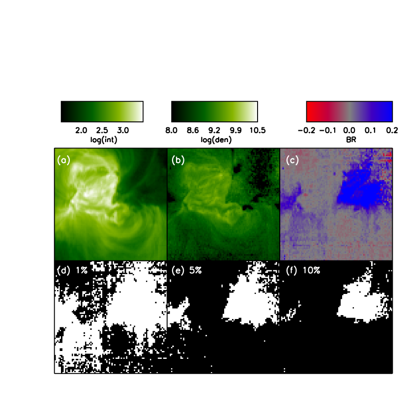
Figure 2: Observations of 11 December 2007 (dataset 8 of Table-1). Panel (a): intensity image for Fe XIV 274 (log scaling). Panel (b): density map from the intensities integrated over the 264 and 274 profiles (log scaling). Panel (c): normalized blue-red asymmetry (c.f. Section 5; linear scaling- positive values (blue) correspond to blue-wing asymmetries; negative values (red) correspond to red-wing asymmetries. Panels (d),(f),(g): binary masks with locations having ${BR}_{norm}>$ 0.01, 0.05 and 0.1 respectively displayed in white. Observed field of view is 256$\times$256 $\mathrm{{arcsec}^{2}}$.

We investigate here in more detail the density content of blue-wing enhancements as anticipated from nanoflare heating. In doing this, we use both analytical theory and time-dependent 1D hydrodynamic simulations. We begin with an analytical derivation.
Analytical derivation
The evaporation velocity and pressure are greatest at or near the end of the nanoflare, depending on whether the heating profile is square-like or triangular-like. Velocity decreases quickly thereafter, because the temperature and heat flux decrease rapidly and because density increases (e.g., Klimchuk, 2006, Fig. 2). Pressure decreases more slowly because the temperature decrease is largely offset by the density increase (only radiation causes the pressure to decrease, and the radiative cooling time is long).

We are interested in the density of the upflow as measured in the blue wings of lines formed at $T\simeq$ 2 MK. Most of this emission comes from the transition region during a time interval immediately following the nanoflare, when density is still increasing. We ignore the flash of emission that occurs as coronal plasma rapidly heats through this temperature early in the nanoflare for the following reasons: it is very temporary, the density is still low, and the velocities are relatively slow.

Because pressure decreases only modestly during the conductive cooling (evaporation) phase, the pressure at the end of this phase (subscript “*”) is approximately equal to the pressure at the time of the blue wing upflow (subscript “b”) (Cargill et al., 2012):

$$P_{*}\approx P_{b}.$$ (4)

Thus,

$$n_{b}\approx n_{*}(T_{*}/T).$$ (5)

The emission in the line core is produced primarily by the coronal plasma as it cools, relatively slowly, through $T$. For lines that are not too hot, this is during the radiative cooling phase that follows the conductive phase. According to Cargill & Klimchuk (2004), there is a $T\propto n^{2}$ scaling during this phase, so the downflow density is

$$n_{c}={(T/T_{*})}^{1/2}n_{*}.$$ (6)

Combining the above two equations we get:

$$n_{b}/n_{c}={(T_{*}/T)}^{3/2}={(T_{*}/T_{m})}^{3/2}{(T_{m}/T)}^{3/2},$$ (7)

where $T_{m}$ is the maximum coronal temperature, at the end of the nanoflare. According to equation (A1) of Cargill & Klimchuk (2004),

$$T_{*}/T_{m}={({\tau}_{c}/{\tau}_{r})}^{1/6},$$ (8)

where ${\tau}_{c}$ and ${\tau}_{r}$ are the conductive and radiative cooling times at the end of the nanoflare. The cooling time ratio is typically in the range ${10}^{-4}<{\tau}_{c}/{\tau}_{r}<{10}^{-2}$ at the end of the nanoflare (Klimchuk et al., 2008; Cargill et al., 2012), so

$$0.22<T_{*}/T_{m}<0.46.$$ (9)

For $T$=2 MK and $T_{m}\in[5,15]$ MK, we have an enhanced blue-wing emission to core density ratio of

$$\frac{n_{b}}{n_{core}}\in[0.4,6.4]$$ (10)

1D Hydrodynamic Nanoflare Simulations
The analytical prediction of Equation 10 is confirmed by 1D hydrodynamic nanoflare simulations. For this task we use the 1D hydrodynamic code called ARGOS, which solves the time-dependent hydrodynamic equations on a adaptively refined grid (Antiochos et al., 1999). We consider semi-circular loops with lengths of 50 and 100 Mm. The selected lengths correspond to typical loop sizes in active region cores and peripheries respectively. The loops are assumed to lie vertically above the solar surface. Initial conditions are determined by calculating static equilibrium solutions with peak temperatures of $\approx$ 0.3 MK and 1 MK. Each initial condition is submitted to a heating pulse with a duration of 50 s and is then allowed to cool down for another 5000 s. We consider heating pulses with different magnitudes leading to maximum temperatures in the range [3.5,17] MK. The impulsive heating for each pulse is uniformly distributed along the modeled loop. The solution of the time-dependent hydrodynamic equations supplies the plasma temperature, density and bulk flow speed as functions of location along the loop and of time. Knowing these physical parameters we produce synthetic profiles for the Fe XIV 264 and 274 lines using CHIANTI. Each profile is given a thermal width from the local temperature and is Doppler-shifted by an amount given by the line-of-sight projection of the local bulk speed. All profiles are calculated in wavelength grids with the same spectral resolution as the blown-up profiles we will describe in Section 5, i.e., 50 times the EIS spectral resolution. In the calculation of the Doppler-shifts, we assume that the modeled loops are viewed from above. The instantaneous profiles are then averaged both in time and space in order to emulate spectroscopic observations of a multi-stranded coronal loop heated by nanoflares. We produce two types of average profiles meant to emulate spectroscopic observations from the footpoint and upper (coronal) parts of a coronal loop. The footpoint profile combines the profiles in the interval spanning from the deepest point in the transition region during each simulation and 10 Mm upwards. Since the location of the transition region is changing in response to pressure changes in the corona during impulsively heated events, selecting the deepest point of the transition region during the entire simulation ensures that the transition region is covered at all times. A coronal profile is constructed from all profiles above the computation region of the footpoint profile until the loop apex. Both footpoint and coronal profiles were averaged over the entire duration of the corresponding simulation. In addition, a ”total” average profile over the entire loop (footpoints and coronal section), is also produced, in order to emulate an unresolved observation combining both footpoint and coronal sections.

We then apply the procedures we describe in Section 5 for the observational data to determine the ratio $R$ of the blue-wing enhancement to the core density from the synthetic profiles resulting from our nanoflare simulations for the footpoint, coronal and ”total” profiles. The applicability of standard spectroscopic diagnostics, like the density-sensitive line ratios used here, to multi-thermal plasmas expected from nanoflare heating was demonstrated by Klimchuk & Cargill (2001). The resulting range of the blue wing to core density ratio is:

$$\frac{n_{b}}{n_{core}}\in[0.44,1.01]$$ (11)

and lies within the interval predicted by the analytical derivation of Equation 10.

Note here that our results above, seem to be insensitive to the spatial localization of nanoflare heating. To check this we perform a set of additional 8 nanoflare simulations with heating concentrated towards the strand footpoints. We consider a 50 Mm long strand at an initial (static equilibrium) temperature of 1 MK. For each simulation, the strand is submitted to a single heating pulse, with an exponential drop-off above the initial location of the transition region. $1/e$ heating lengthscales of 1000 and 5000 km are used. The simulated nanoflares reach maximum temperature in the range 3-12 MK. The $n_{b}/n_{core}$ ratio takes values in the interval 0.55-1.2, which is similar to the range obtained for uniform heating.

Before proceeding to compare our theoretical predictions with observations, we note the blue wing to core density ratios predicted for type II spicules (Equation 3) and coronal nanoflares (Equations 10 and 11) are greatly different. The ranges do not overlap. Consider the upward flow of hot material crossing an imaginary surface in the low corona. The time-integrated mass flux must equal all of the coronal material that ultimately fills the strand. In the case of a spicule, the material crosses the surface very quickly. The crossing time scale is just the thickness of the hot spicule tip divided by the upflow velocity, which is about 10 s. Evaporation, on the other hand, is a process that continues for a much longer time. Since the velocity is similar (we measure a particular wavelength band in the blue wing), the density must be inversely proportional to the time scale in order to get the same total mass. Hence, the density is much smaller for evaporation than for spicules. It is unreasonable to expect that the uncertainties and limitations in the determinations of the density ratios would bridge the significant gap. This makes the upflow to core density ratio an important and sensitive diagnostic means for studying the source of high-speed coronal upflows.

3 Observations

We use spectroscopic observations taken by the Extreme Ultraviolet Imaging Spectrometer (EIS), Culhane et al. (2007), on-board the Hinode mission. EIS is a normal incidence spectrometer taking observations in two wavelength ranges in the Extreme Ultraviolet: 170-210 Å  and 250-290 Å. These ranges cover lines formed in the chromosphere, transition region and corona. EIS has spectral pixels of 22 mÅ, corresponding to $\approx$ 25 $\mathrm{km\,{s}^{-1}}\,$and a spatial resolution of about 2 arcsec. For more on EIS we refer to Culhane et al. (2007).

The observations we analyze here were taken during the period 2006-2007 and correspond to several two-dimensional spectral scans (rasters) over active regions at various locations on the solar disk. Detailed spectra of various selected spectral lines at each spatial location covered by the raster scan are obtained. More information (e.g., time of observation, size of raster, location of raster etc) for each observation is supplied in Table-1. The level0 data were submitted to the standard data reduction pipeline for EIS data using the eis_prep.pro routine.

4 The Fe XIV (264/274) Density Sensitive Ratio

The intensity ratio of the Fe XIV lines at 264.78 and 274.20, hereafter 264 and 274, represents a good density diagnostic for coronal plasmas. All atomic physics calculations and diagnostics used in this paper use the latest version (v7.1, Landi et al. (2013)) of CHIANTI (Dere et al., 1997).

The solid line of Figure 1 shows the theoretical 264 to 274 intensity ratio against density for the formation temperature of Fe XIV (6.3 in log(T)). This curve is used throughout this study for all density calculations and we call it our standard diagnostic curve. The 264/274 intensity ratio is sensitive to density for the interval $\approx$ [0.65,2.9] which corresponds to densities in the range $\approx{10}^{8}-{10}^{12}\mathrm{{cm}^{-3}}$. However, the region of higher sensitivity corresponds to ratios in the more compact ratio range of $\approx$ [0.9,2.6] and conversely to densities in the range of $\approx[2\times{10}^{9},4\times{10}^{10}]\mathrm{{cm}^{-3}}$. For intensity ratios approaching the lower or the upper limit of the former interval, where the density sensitivity on the line ratio becomes much smaller (i.e., the density-ratio curve becomes almost flat), one can only deduce an upper, $n_{max}$ =${10}^{8}$ $\mathrm{{cm}^{-3}}$or lower $n_{min}={10}^{12}$ $\mathrm{{cm}^{-3}}$  limit on the density respectively. Note here that one should not over-intepret these densities and their values; cases with densities equal to $n_{max}$ or $n_{min}$ are simply telling us that the corresponding intensity ratio measurements are below/above the low/high limits respectively.

A potential burden in the analysis of the weak wing emissions of spectral lines, which is the focal point of this study, could arise from the presence of line blends, i.e., ”parasitic” lines close to the ”target” lines. Line blends may affect the intensities of the ”target” lines. Inspection of published EIS line lists, based on both atomic physics calculations and observations shows that the two Fe XIV lines of interest are largely free of blends (e.g., Young et al., 2007; Brown et al., 2008; Del Zanna, 2012). However, there exist two lines close to the centers of the two Fe XIV lines that warrant meticulous consideration. First, there is a Si VII line at 274.18 Å , or $\approx$ 22 $\mathrm{km\,{s}^{-1}}\,$towards the blue of the 274 Fe XIV rest wavelength. Second, there is a Fe XI line at 264.77 Å , or $\approx$ 18 $\mathrm{km\,{s}^{-1}}\,$towards the blue of the 264 Fe XIV rest wavelength. These lines are not very far from the cores of the Fe XIV lines of interest, but they may nevertheless affect their wing intensities. For example (Landi & Young, 2009) found that the Si VII line contributes 57$\%$ to the observed fan loops in an AR.

Fortunately, the Si VII and Fe XI blends have known intensity ratios with a Si VII line at 275.35Å  and a Fe XI line at 188.23Å  respectively (e.g., Young et al., 2007). These two lines can be observed by EIS. Moreover they are isolated and thus their intensities can be measured accurately. For typical coronal densities the Fe XI 264.77/188.23 ratio varies between about 0.026 to 0.043; therefore measuring the Fe XI 188.23 Å intensities and multiplying them by 0.043 supplies an upper limit on the contribution of the Fe XI 264.77 line to the Fe XIV 264 line. Similarly, the Si VII 274.2/275.35 intensity ratio has a maximum value of 0.25; therefore multiplying the Si VII 275.35 intensity by 0.25 supplies an upper limit on the contribution of the Si VII 274.2 line to the Fe XIV 274 line.

Observed cases for which the Fe XI and Si VII blends are simultaneously $\leq 10\%$ of the measured intensities of the Fe XIV 264 and 274 lines respectively were selected for further analysis since the blend contribution to the ”target” line core and wing intensities can be rather safely neglected. As discussed before, both line blends are only slightly offset and roughly at the same distance from the rest wavelength positions of the ”target” lines. Therefore, given our selection criterion, they should amount at maximum to no more than the $10\%$ of the ”target” line core. The blends will contribute an even smaller percentage to the line wings if the flows that produce the wing emission have a temperature dependence such that cooler plasma is also slower. This will be the case for evaporated plasma, where $v\propto T$, though not necessarily for spicules. The cases where the $10\%$ criterion is satisfied for both Fe XIV lines are referred to as “No-Blend” (second column in Table 2). On average, the blend contribution for the cases not satisfying the above criterion for the ”base” observation discussed later on in the paper correspond to 16 $\%$ and 19 $\%$ of Fe XIV 264 and 274 intensities respectively. The average intensity contributions of Fe XI and Si VII to the 264 and 274 features across all the active region raster of the ”base” observation are 7 $\%$ and 4$\%$, respectively.

We now consider the potential impact of our ”No-Blend” criterion on the density diagnostic. First consider the case when the Fe XI and SI VII blends amount to exactly the same fraction of the 264 and 274 lines respectively, then they will not influence the density diagnostic at all: i.e. the standard diagnostic curve of Figure 1 will not be affected. Allowing for a blend contribution of a maximum value of 10 % in either the 264 or the 274 intensity will lead to an overestimate or underestimate of the 264/274 intensity ratio by a factor of 0.1 respectively. In Figure 1 we show diagnostic curves corresponding to these two extreme cases: long-dashed and dashed-triple-dotted corresponding to 1.1 and 0.9 of the standard diagnostic curve. When the 264 and 274 blends represent a smaller, yet non-equal amount of these lines, their contribution to the density diagnostic will be bounded between the two extreme cases considered above: i.e., the corresponding diagnostic curves will be between the long-dashes and dashes-triple-dots of Figure 1.

We can now evaluate the impact of the blend on the density diagnostic. Take an intensity ratio of 1.1. The standard curve for this ratio yields a typical AR density of about 2$\times{10}^{9}$ $\mathrm{{cm}^{-3}}$. Allowing for a maximal blend contribution of 10 % of either the 264 or the 274 line (i.e., the long-dashed and the dashed-double-dotted curves of Figure 1 respectively) leads to an overestimate or underestimate of the density by a factor of less $\approx$ 2 (we use the standard curve in all density calculations). Similar discrepancy factors can be found if we consider other values for the line ratio. Note that these underestimate/overestimate factors represent generous upper limits.

As discussed before the standard density diagnostic curve of Figure 1 was determined using the temperature of peak Fe XIV formation under equilibrium ionization conditions (log(T)=6.3). However, it is possible that the plasma is at a different equilibrium temperature or that the plasma is rapidly heating as it rises or rapidly cooling as it descends. Therefore, the actual temperature at the time Fe XIV is present could be different from the equilibrium temperature. We thus calculated the theoretical 264 to 274 intensity ratio for log(T)=6.5 and log(T)=6.1 long-dashes and dashed-dots of Figure 1 respectively. These temperature correspond to the upper(lower) end of the $FWHM$ range of the Fe XIV contribution function. From Figure 1 we have that a hotter upflowing plasma leads to an overestimate of the density with respect to the standard density diagnostic curve, but by a rather small factor (much less than 2). The opposite (underestimating the density) occurs when considering warmer, downflowing plasmas (dashed curve in Figure 1). Again, the deviation from the standard diagnostic curve is rather small.

To sum up, we conclude that the possible contribution of (known) line blends and departures from the formation temperature of Fe XIV leads to density uncertainties of a factor of 2.

Before proceeding, we note that other coronal density sensitive line ratios available in EIS observations, Fe XII 196.64/195.12 and Fe XIII 203.82/202.04, exhibit also blending issues or have other strong lines in their vicinities that need to be treated simultaneously (e.g., Young et al., 2007).

5 Analysis Method

We are now set to describe the method we use to calculate the density associated with excess blue or red wing emissions which correspond to fast upflowing or downflowing plasmas respectively. These densities will then be compared with those of the line core corresponding to almost static plasmas. To increase the signal-to-noise (S/N) ratio, we calculated averaged line profiles over 3$\times$3 full resolution pixels. It is important to have sizeable S/N ratios since we wish to obtain detailed measurements at the line wings, where intensities are low.

For all macropixels satisfying the ”No-Blend” criterion of the previous Section we proceed as follows:

• interpolate each 264 and 274 Fe XIV profile and the associated intensity errors (arising from photon-counting statistics and readout noise) onto a 50 times finer grid using an improved cubic-spline interpolation scheme. The scheme, fully described in Klimchuk, Patsourakos and Tripathi (2013), addresses the important fact that while the intensity we observe in a spectral bin is the mean intensity averaged over the bin, traditionally it is assigned to the bin center. This is only appropriate, however, if the line profile within the bin is symmetric about the bin center (e.g., a straight line segment), which is generally not the case. The true bin center intensity is generally different from the bin average, and not taking this into account can impact the very delicate measurements of wing intensities and line center locations we hereby perform. The new scheme, based on an iterative method, rapidly converges to solutions conserving the total intensity across the bin. It is therefore called Intensity Conserving Spline Interpolation (ICSI).

• determine the wavelength location of peak intensity which is assumed to correspond to a zero Doppler-shift;

• determine the integrated intensity of the blown-up (50 times higher resolution) profiles for their blue ([-150,-50] $\mathrm{km\,{s}^{-1}}\,$from peak intensity location) and red ([50,150] $\mathrm{km\,{s}^{-1}}\,$from peak intensity location) wings: $i_{blue}$ and $i_{red}$ respectively;

• determine the residual wing intensity $i_{diff}=i_{blue}-i_{red}$ for both Fe XIV lines;

• if $i_{diff}$ has the same sign for both lines, i.e. both Fe XIV lines exhibit a blue-wing or red-wing asymmetry, then use the corresponding $i_{diff}$ to determine the corresponding density $n_{diff}$ from the $I_{264}/I_{274}$diagnostic of Section 4;

• subtract a linear background from the blown-up profiles and determine the core intensity $i_{core}$ in the [-30,30] $\mathrm{km\,{s}^{-1}}\,$interval centered at the peak intensity location, and the associated density $n_{core}$ from the $I_{264}/I_{274}$diagnostic of Section 4;

• deduce a blue-red asymmetry, $BR=i_{diff}$, and its normalized to the core intensity version, $BR_{norm}=i_{diff}/i_{core}$;

• determine the density ratio, $rat=n_{diff}/n_{core}$ between excess wing and core emissions.

Profiles with positive $BR$ correspond to a blue-wing enhancement while those with negative $BR$ to a red-wing enhancement. Similar analysis methods to deduce profile asymmetries are commonly used (e.g. De Pontieu et al., 2007). Note here that a significant number of profiles corresponds to residual intensities, $i_{diff}$ with $264/274$ ratios lying outside the density sensitive part of the $n-264/274$ curve discussed in Section 4. For these profiles we are only able to deduce an upper (${10}^{8}\mathrm{{cm}^{-3}}$) or a lower (${10}^{12}\mathrm{{cm}^{-3}}$) density limit.

An underlying assumption in our analysis is that, by differencing the two sides of the line profile, we are isolating the emission of rapidly flowing plasma from the wing emission of rest material. This is strictly correct only if fast material contributes to just one side of the profile, i.e., is only flowing up or down. The assumption is nonetheless reasonable if there are both upflows and downflows as long as the enhanced emission is substantially brighter in one wing than the other. We find that $n_{diff}$ is not well correlated with either the magnitude or sign of ${BR}_{norm}$, suggesting that measurements are a good indication of the actual density of the dominant high-speed material.

Note here that in the calculation of the $n_{diff}/n_{core}$ ratio any systematic error, e.g. instrument calibration and atomic physics, cancels out since it has the same sign for each calculated density. Moreover, and since we are interested in a density ratio, it may be that the impact of the line blends of the 264 and 274 lines discussed in Section 4 could cancel out as well. This is because, as discussed in Section 4 both blends are at similar wavelength locations with respect to the line of interest and therefore it is possible they may affect the wing and core intensities and thus densities in a similar manner. At any rate, we need to consider the maximum uncertainty factor of $\approx$ 2 in the inferred densities from (known) line blending we deduced in Section 4.

We therefore need to consider only the effect of random errors in $n_{diff}/n_{core}$ ratio. Uncertainties in the resulting histograms are deduced with the following bootstrapping method. For a number of realizations (=1000) we randomly perturb the density ratios for a random sample of $N$macropixels, where $N$ is the total number of macropixels and determine the corresponding histogram. We then determine the average and standard deviations of the resulting histograms for the 1000 realizations. The pertubations in the density ratios take into account standard errors and error propagation.

6 Results

We now present the results of our analysis. Take as example the observation which took place on 11 December 2007 (dataset 8 of Table 1); we call this observation our base observation. We will nevertheless supply all the important information regarding all considered observations. In Figure 2 we show the 274 Fe XIV image (panel a), the density map from the profile-integrated 264 and 274 intensities using the density diagnostic of Section 4 (panel b), and the normalized $BR$ asymmetry as defined in the previous Section (panel c). From the 274 image we note we are dealing with a small bipolar AR. Densities are enhanced in the AR core, and they decrease when going to its periphery. Most of the observed field contains profiles with $BR>0$, in other words with enhanced blue-wing emission, in agreement with previous studies. The blue-wing asymmetries are stronger at the edges of the AR (dark areas in the 274 intensity image), although they can be also seen in the AR core. There are finally fewer locations with red-wing enhancements ($BR<0$). Note here, and also found in other studies, that the observed asymmetries are rather weak. For example, for profiles with $BR>0$, the average $BR_{norm}$ is only 0.04; 76$\%$ of the profiles have $BR_{norm}>0.01$. To illustrate this furthermore, panels (e),(f) and (g) in Figure 2 contain binary masks with the locations, shown in white, of 274 profiles having $BR_{norm}>$ 0.01, 0.05 and 0.1 respectively. It is obvious that locations with sizeable $BR_{norm}$ (i.e., $>0.05$ for example) are signficantly fewer than those corresponding to the full $BR_{norm}$ distribution.

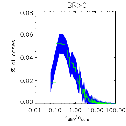
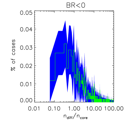
Figure 3: Histograms (green histogram-mode lines) and 2-$\sigma$ uncertainties (blue contours) of $n_{diff}/n_{core}$ for the observation of 11 December 2007. Locations with positive blue-red (left panel) and negative blue-red asymmetry (right panel).

In the left panel of Figure 3 we plot the histogram of $n_{diff}/n_{core}$ for points with $BR>0$ of the base observation as determined by the procedure described in Section 5. In this case $n_{diff}$ is equal to $n_{b}$, the density of the blue-wing enhancement. The peak of the distribution is below 1 ($\approx$ 0.2) signifying that the most probable density of the blue-wing enhancement is smaller than that of the line core. The median value of the distribution is slightly above 1 (2.2). These findings are consistent with the predictions for coronal nanoflares using both analytical (Equation 10) and numerical (Equation 11) approaches. On the other hand, the density ratios are much smaller than predicted for type II spicules. If spicules supply most of the hot plasma in the corona, then $n_{diff}/n_{core}$ must be significantly larger than 1 ($>>$ 16.6): see Equation 3). It may be that the observed blue wing emission does in fact come from spicules and has a density $n_{diff}=n_{b}$, but the density of this material will be far less than $n_{core}$ after it has expanded to fill the loop strand. In that case, the observed $n_{core}$ represents material not associated with spicules (e.g., evaporated material produced by coronal nanoflares). We note that a small minority of density ratios at the tail of the distribution, having large ($>>1$) $n_{diff}/n_{core}$, are consistent with type II spicules being the dominant source of hot plasma at those locations.

The two leftmost panels of Figure 4 show results for macropixels with $BR>0$ in the base observation where only an upper limit (first panel) or a lower limit (second panel) could be determined for the blue-wing enhancement, as discussed in Section 4. Cases with blue-wing enhancement density equal to an upper limit $n_{max}$ =${10}^{8}$ $\mathrm{{cm}^{-3}}$are not consistent with type II spicules since this density is smaller than the corresponding core density (1st panel of Figure 4). On the other hand, cases with blue-wing enhancement density equal to a lower limit $n_{min}={10}^{12}$ $\mathrm{{cm}^{-3}}$are consistent with type II spicules since they correspond to blue-wing enhancement to core density ratios much higher than 1 (2nd panel of Figure 4). Interestingly, EIS observations of coronal jets show elevated blue wing densities in the range found above (Chifor et al., 2008). We defer a discussion of results from macropixels with negative $BR$ asymmetry displayed in Figures 3 and 4 for the next Section.

In order to relate how the densities associated with excess wing emissions depend on different solar features within the observed ARs, we display in Figure 5 the variation of $n_{diff}/n_{core}$ as a function of $n_{core}$ for locations exhibiting $BR>0$ (upper panel) and $BR<0$ (lower panel). The plot corresponds to the base observation. Locations with low $n_{core}$ correspond to low-emitting structures that can be found in AR edges, while locations with high $n_{core}$ correspond to AR cores. From Figure 5 we note a trend of decreasing $n_{diff}/n_{core}$ with increasing $n_{core}$ for locations with both $BR<0$ and $BR>0$.

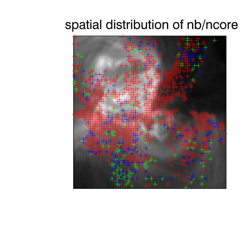
Figure 6: Spatial distribution of $n_{b}/n_{core}$ for the following ranges: $\leq 6.4$ (red crosses), $\geq 16.6$ (green crosses) $\in(6.4,16.6)$ (blue crosses), overplotted on the corresponding 274 image. Data correspond to the base observation.

As a further illustration of the spatial distribution of the density ratio, Figure 6 contains $n_{diff}/n_{core}$ for profiles with $BR>0$ for different ranges. We can note that profiles with high $n_{diff}/n_{core}$ (green crosses), which are consistent with spicules, are located mostly at the observed AR edges, although there are also a few cases in the AR core. The more numerous profiles, with low $n_{diff}/n_{core}$ values (red crosses), which are consistent with nanoflares, occur both in the AR core and at its edges. A similar behavior applies to profiles with intermediate $n_{diff}/n_{core}$ values (blue crosses).

Having available the densities of the excess wing emissions and of the line cores we are able to calculate the formation path lengths of the corresponding emissions. We first note that the intensity of neither 264 nor 274 has a $n^{2}$ dependence: the intensities of both lines are $\propto$ $n^{2+\alpha}$ with $\alpha>0$ for 274 and $\alpha<0$ for 264. It is indeed because of these dependencies that the intensity ratio of 264 and 274 is density-sensitive. However, the sum of the 264 and 274 intensities does almost have an exact $n^{2}$ dependence. We can therefore write that:

$$I_{264}+I_{274}=F(T)n^{2}\phi dl,$$ (12)

where $I_{264}$ and $I_{274}$ correspond to the 264 and 274 intensities respectively of a particular spectral feature (excess wing emission or core), $F(T)$ is the sum of the contribution functions of 264 and 274 calculated at the formation temperature of Fe XIV multiplied by the iron abundance, and $dl$ is the line-of-sight thickness of the volume containing emitting material, and $\phi$ is the filling factor of that material. For blue wing observations near disk center, $dl$ is either the thickness of the transition region (for a nanoflare) or the length of the hot section of the spicule, and $\phi$ is the fractional area of the unresolved strands that are experiencing either nanoflare evaporation or spicule ejection. For line core observations, $dl$ is the scale height of the emission (thickness of the corona) and $\phi$ is fractional volume of the strands that contain plasma at that temperature (2 MK in this case).

We applied Equation 12 to the line core and excess wing intensities and densities to deduce $\phi dl$. Figure 7 contains the results for the core (upper panel) and the excess wing emission (lower panel) for $BR>0$ for the base observation. We note that the excess wing emissions have significantly smaller $\phi dl$ compared to the line cores, with the corresponding distributions peaking at $\approx$ 300 km and 4000 km respectively. The latter is comparable to diameters of macroscopic coronal loops (e.g., Peter et al., 2013); even longer $\phi dl$ of the line cores could correspond to diffuse corona regions, with very long lines of sight. The much smaller formation lengths of the excess blue-wing emissions hint on small-scale possibly time-dependent processes. Both type II spicules (e.g., De Pontieu et al., 2009) and nanoflares involve small spatial scales.

7 Summary and Discussion

The main aim of this work is to establish the density content of enhanced wing emissions far off ($\mid\delta v\mid\in[50,150]$ $\mathrm{km\,{s}^{-1}}\,$) the line centers and to compare it with that of the line cores ($\delta v\in[-30,30]$ $\mathrm{km\,{s}^{-1}}\,$), and particularly for cases corresponding to blue-wing enhancements. Our main conclusions from the previous Sections are:

1. the bulk of the $n_{b}/n_{core}$ distribution, where both quantities can be measured, (e.g., Figure 3) corresponds to too low values to be consistent with the view that type II spicules are the primary source of hot plasma in the corona.

2. the values are consistent with the predictions for coronal nanoflares.

3. cases in the tail of the $n_{b}/n_{core}$ distribution (e.g., Figure 3) are consistent with type II spicules since they correspond to high $n_{b}/n_{core}$ values. The same applies to cases with blue-wing enhancement density corresponding to the lower density limit (e.g., Figure 4). Both these cases correspond though to a small fraction of macropixels (for example the latter corresponds to only the 2.9 $\%$ of macropixels of the base observation).

4. cases for which only an upper limit to the blue-wing enhancement density can be estimated (e.g., Figure 4) account for a significant fraction of the total number of macropixels (14.6 $\%$ for the base observation). These low density values are not consistent with type II spicules.

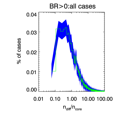
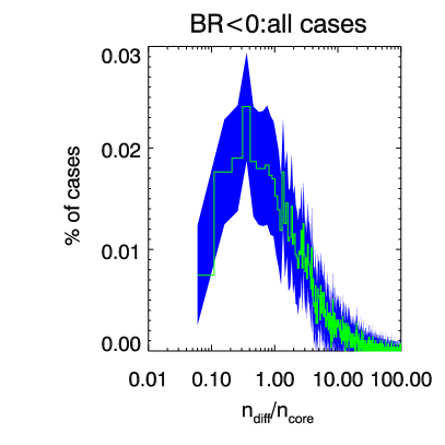
Figure 8: Histograms (green histogram-mode lines) and 2-$\sigma$ uncertainties (blue contours) of $n_{diff}/n_{core}$ for the all analyzed datasets. Locations with positive blue-red (left panel) and negative blue-red asymmetry (right panel).

Our conclusions above can be extended to a larger statistical sample containing 7 more AR datasets on-top of the base observation (see Table-1, Table-2 and Table-3). Take for example Figure 8 where we show the $n_{b}/n_{core}$ histogram for the 8 analyzed datasets. Once more we note that the bulk of the $n_{b}/n_{core}$ distribution corresponds to small blue-wing densities, with again a high $n_{b}/n_{core}$ tail. Similar results to the base observation apply also to cases where the lower or upper density limit of the blue-wing enhancement is reached. Indeed, if spicules are dominant, then one would expect to see most of the wing densities to be very high, i.e., reaching the lower density limit. The result however (column I of Table 2) is that very few pixels (1.7-3.5 $\%$) actually reach very high densities. We therefore conclude from the present analysis that type II spicules are consistent with a only small fraction of the considered cases and thus their potential for supply of the bulk of the coronal mass in ARs seems rather limited. This is consistent with two recent studies. In Brooks & Warren (2012) the emission measure of the fast upflowing plasma was found to strongly peak at coronal temperatures (1.2-1.4 MK), while it was almost an order of magnitude smaller at transition region temperatures (0.6 MK). This finding was interpreted as the plasma producing the asymmetries having coronal origin and possibly not being directly ejected from below and heated on the fly. Brooks and Warren made their measurements in the faint periphery of an active region, where the BR asymmetries are greatest. Tripathi & Klimchuk (2013) recently obtained similar results in the bright core of an active region. Moreover, Klimchuk (2012) used several independent arguments, including ones based on the line asymmetry and on the ratio of emission measures in lower transition region and corona, to conclude that type II spicules provide only a small fraction ($<$ 2 $\%$) of the hot plasma observed in the AR corona.

We now pass on to a discussion concerning cases with enhanced red-wing emissions (i.e., $BR<0$). They represent a significant, yet smaller, fraction compared to cases with $BR>0$ (for example they correspond to 14.5 $\%$ of the total number of cases or about the half of the cases with $BR>0$). The $n_{r}/n_{core}$, $n_{r}$ is the red-wing enhancement density, distributions peak at around 1 for both the base observations and the ensemble of the 8 AR observations, right panels of Figures 3 and 8 respectively. There are only few cases at the high-ratio tails of the $n_{r}/n_{core}$ distributions for which $n_{r}$ is much larger than $n_{core}$. Finally, similar results to the $BR>0$ case, are obtained for profiles with densities equal to the upper and lower density limit (see for example panels 3 and 4 of Figure 4).

What could be then the physical mechanism causing these red-wing enhancements? ”Standard” mass draining taking place during the radiatively dominated cooling phase of cycles of impulsive heating and cooling cannot possibly account for these enhancements. This is because the predicted downflow speeds typically barely exceed $\approx$ 20 $\mathrm{km\,{s}^{-1}}\,$, which is much smaller than the speed of the inferred downflows $>$50 $\mathrm{km\,{s}^{-1}}\,$. An attractive possibility to generate high-speed downflows can be catastrophic cooling and coronal rain (e.g. Antiochos et al., 1999; Karpen et al., 2001; Müller et al., 2004; Karpen & Antiochos, 2008; Mok et al., 2008; Antolin et al., 2010) The essence of this mechanism is that highly concentrated heating at the feet of coronal loops increases the coronal density until the coronal radiative losses cannot any more be supported by (the weak) coronal heating. This triggers a run-away catastrophic cooling and high-speed downflows, and speeds as high as $\approx$ 100 $\mathrm{km\,{s}^{-1}}\,$are predicted. The observational signature of catastrophic cooling is thought to be the coronal rain, which consists of high-speed downflowing blobs observed off-limb (e.g. Schrijver, 2001). Current estimates of the fraction of the coronal volume occupied at any given time by coronal rain are rather uncertain since they are carried out in off-limb observations, with the inherent influence of projection effects (Antolin & Rouppe van der Voort, 2012). On the other hand, observing coronal rain on the disk is a more promising avenue for determining the discussed above coronal rain filling factor, although plagued by the low visibility of the associated blobs against the disk background (Antolin et al., 2012). Coordinated disk observations of coronal rain and of line asymmetries in coronal lines could help.

Our study, along with any other aiming at the wings of spectral lines, is arguably pushing the analysis and the interpretation of current spectroscopic observations to their limits. For example with this study we took the utmost caution to minimize the impact of any known blend for the two Fe XIV lines used in the density determinations. This requirement already eliminates a significant fraction of pixels from further analysis ($\approx$ 11.1-58.2 % of the pixels of the 8 analyzed datasets; see column B of Table-2). Moreover, there is a significant fraction of pixels with inconsistent sign of $BR$ asymmetry for the two Fe XIV lines ($\approx$ 18.4-35.9 % of the pixels of the 8 analyzed datasets; see columns E and F of Table-2). This implies the presence of some identified blends at the line wings or maybe the impact of low S/N at line wings. The main reason that blends and/or noise force us to exclude many pixels from our measurements is that the excess wing emission is extremely faint. Klimchuk (2012) used this fact to conclude that type II spicules are not a dominant source of hot coronal plasma. All the above is essentially telling us that we cannot use measured densities to comment on the source of the coronal mass for a significant fraction ($\approx$ 42.0-78.3 % of the pixels of the 8 analyzed datasets; see columns B,E,F in Table-2) of the observed pixels. Moreover, the wavelength sampling of EIS observations is rather coarse when performing studies of the fine and subtle details of spectral line profiles. A typical line profile (core and wings) comprises no more than about 12 EIS spectral pixels which make it difficult to resolve blends and to generally work on wing emissions. Increasing the wavelength sampling and the sensitivity of spectroscopic observations may help into increasing the number observational pixels with useable wing emissions.

Another potential limitation of the present study is that our density calculations are based on the assumption of ionization equilibrium. Such an assumption is possibly suspect when dealing with fast flowing plasmas associated with either type II spicules or nanoflares given that they are formed under rapidly varying physical conditions involving time-dependent heating and flow through steep temperature gradients (e.g. Bradshaw & Cargill, 2006; Reale & Orlando, 2008; Bradshaw & Klimchuk, 2011). Detailed calculations of density-sensitive ratios of fast flowing plasmas under dynamic conditions, taking into account possible departures from ionization equilibrium, are required to determine the precise impact of such effects on the corresponding diagnostics. Indeed, this important task has been recently undertaken in Doyle et al. (2012) and Olluri et al. (2013), where density diagnostics for the intensity ratio of two transition region lines of O IV was calculated for dynamic events. The inclusion of non-equilibrium ionization led to significant deviations of the resulting densities (up to an order of magnitude underestimate) with respect to the values calculated under ionization equilibrium conditions.

Next generation sub-arcsecond class spectrometers with chromosphere-transition region-corona coverage like the Interface Region Imaging Spectrometer (IRIS; Wülser et al. (2012)) the Very High Angular Resolution Imaging Spectrometer (VERIS; Korendyke et al. (2007)) and the Large European Module for solar Ultraviolet Research (LEMUR; Teriaca et al. (2012)) are expected to significantly advance our understanding of the flow of the mass and heat in the solar atmosphere. For example, their sub-arcsecond resolution would allow to spectroscopically resolve type II spicules in the plane of the sky, i.e., observe a distinct spectroscopic component and not merely a weak wing enhancement. This separation would allow to take better measurements of their physical parameters (densities, emission measures, abundances, etc) and compare them with the plasma bulk. However, there is always the inherent problem of LOS integration, so the spicule emission will be mixed with all the other emission in front of it.

Table 1: General information of the analyzed datasets.

Dataset	Date	Time (UT)	Location (arcsec from Sun center)	Field of View Size
1	1 December 2006	00:24:16	(-198,-141)	255$\times$255
2	2 December 2006	10:33:23	(203,-185)	255$\times$255
3	20 Janurary 2007	02:33:52	(347,9)	255$\times$255
4	1 February 2007	00:12:12	(-185,-141)	255$\times$255
5	2 May 2007	05:27:17	(122,-132)	240$\times$240
6	1 July 2007	04:56:57	(-112,-215)	240$\times$240
7	24 August 2007	01:18:05	(-755,-169)	255$\times$255
8	11 December 2007	00:24:16	(-198,-141)	255$\times$255

Table 2: Macropixel statistics. All columns except the first supply percentages over the total number of macropixels in each dataset.

A	B	C	D	E	F	G	H	I
Dataset	“No” Blend	B &	B&	B &	B &	C(D) &	C(D) &	C(D) &
Number		$I_{B}>I_{R}$	$I_{B}<I_{R}$	$I_{B}>I_{R}$	$I_{B}>I_{R}$	measurable $n_{diff}$	high $n_{diff}$	low $n_{diff}$
		both lines	both lines	264 only	274 only
							limit	limit
1	52.3	21.2	11.7	6.1	13.2	8.9(5.1)	10.3(3.9)	1.7(2.6)
2	72.3	28.2	14.5	7.2	22.3	12.3(6.8)	13.2(4.7)	2.5(2.9)
3	58.6	29.6	8.8	7.0	12.9	13.1(3.9)	13.3(2.4)	3.1(2.4)
4	75.9	30.4	13.6	7.7	24.0	11.5(6.6)	15.2(3.1)	2.5(3.5)
5	65.0	22.0	13.0	7.5	22.3	8.6(6.0)	10.2(3.5)	2.5(3.2)
6	41.8	12.8	8.8	7.1	13.0	5.0(3.2)	4.2(2.3)	2.4(2.8)
7	88.9	34.6	18.3	11.5	24.4	13.7(7.5)	12.3(5.0)	3.5(4.1)
8	76.4	41.3	16.6	9.1	9.3	22.7(8.4)	14.6(5.5)	2.9(2.5)

Table 3: Statistics of $n_{diff}/n_{core}$ for cases corresponding to the entries of column G of Table 2, i.e. macropixels where $n_{diff}$ and $n_{core}$ can be measured and BR is positive or negative (in parentheses) for both 264 and 274.

Dataset Number	Peak of distribution	Median of distribution	$FWHM$ of distribution
1	0.4(1.0)	2.69(5.3)	0.9 (0.9)
2	0.6(2.8)	2.2(4.4)	1.3(2.3)
3	0.7(0.1)	2.8(5.4)	0.9(1.7)
4	0.4(0.3)	3.9(4.3)	1.3(1.5)
5	0.8(0.2)	3.3(4.3)	1.3(0.8)
6	0.1(1.1)	3.0(8.9)	0.4(1.2)
7	0.5(0.3)	4.9(6.8)	1.3(0.4)
8	0.1(0.3)	1.6(3.3)	1.0(1.2)

Figure 1: Fe XIV 264/274 density diagnostic. Solid line: standard curve used in all calculations for the formation temperature of Fe XIV (6.3 in log(T)); short-dashes: log(T)=6.1; dashes-dots: log(T)=6.5; dashed-triple-dots: 0.9*standard curve; long-dashes:1.1*standard curve.

  

  

Figure 4: Histograms $n_{max}/n_{core}$ and $n_{min}/n_{core}$ for the observation of 11 December 2007. Two left-most (right-most) panels correspond to cases with positive (negative) blue-red asymmetry.

Figure 5: $n_{diff}/n_{core}$ versus $n_{core}$ for profiles exhibiting $BR>0$ (upper panel) and $BR<0$ (lower panel). Data correspond to the base observation.

Figure 7: Histograms of formations lengths for cases with $BR>0$ in the base observation. Upper panel has the results for $n_{core}$ and lower panel for $n_{diff}$.

References

- Antiochos et al. (1999) Antiochos, S. K., MacNeice, P. J., Spicer, D. S., & Klimchuk, J. A. 1999, ApJ, 512, 985
- Antolin et al. (2010) Antolin, P., Shibata, K., & Vissers, G. 2010, ApJ, 716, 154
- Antolin & Rouppe van der Voort (2012) Antolin, P., & Rouppe van der Voort, L. 2012, ApJ, 745, 152
- Antolin et al. (2012) Antolin, P., Vissers, G., & Rouppe van der Voort, L. 2012, Sol. Phys., 280, 457
- Beckers (1972) Beckers, J. M. 1972, ARA&A, 10, 73
- Bradshaw & Cargill (2006) Bradshaw, S. J., & Cargill, P. J. 2006, A&A, 458, 987
- Bradshaw (2008) Bradshaw, S. J. 2008, A&A, 486, L5
- Bradshaw & Klimchuk (2011) Bradshaw, S. J., & Klimchuk, J. A. 2011, ApJS, 194, 26
- Brooks & Warren (2012) Brooks, D. H., & Warren, H. P. 2012, ApJ, 760, L5
- Brown et al. (2008) Brown, C. M., Feldman, U., Seely, J. F., Korendyke, C. M., & Hara, H. 2008, ApJS, 176, 511
- Bryans et al. (2010) Bryans, P., Young, P. R., & Doschek, G. A. 2010, ApJ, 715, 1012
- Cargill (1994) Cargill, P. J. 1994, ApJ, 422, 381
- Cargill & Klimchuk (2004) Cargill, P. J., & Klimchuk, J. A. 2004, ApJ, 605, 911
- Cargill et al. (2012) Cargill, P. J., Bradshaw, S. J., & Klimchuk, J. A. 2012, ApJ, 752, 161
- Cargill et al. (2012) Cargill, P. J., Bradshaw, S. J., & Klimchuk, J. A. 2012, ApJ, 758, 5
- Chifor et al. (2008) Chifor, C., Young, P. R., Isobe, H., et al. 2008, A&A, 481, L57
- Culhane et al. (2007) Culhane, J. L., Harra, L. K., James, A. M., et al. 2007, Sol. Phys., 243, 19
- De Pontieu et al. (2007) De Pontieu, B., McIntosh, S., Hansteen, V. H., et al. 2007, PASJ, 59, 655
- De Pontieu et al. (2009) De Pontieu, B., McIntosh, S. W., Hansteen, V. H., & Schrijver, C. J. 2009, ApJ, 701, L1
- De Pontieu et al. (2011) De Pontieu, B., McIntosh, S. W., Carlsson, M., et al. 2011, Science, 331, 55
- Del Zanna (2012) Del Zanna, G. 2012, A&A, 537, A38
- Dere et al. (1997) Dere, K. P., Landi, E., Mason, H. E., Monsignori Fossi, B. C., & Young, P. R. 1997, A&AS, 125, 149
- Dolla & Zhukov (2011) Dolla, L. R., & Zhukov, A. N. 2011, ApJ, 730, 113
- Doschek (2012) Doschek, G. A. 2012, ApJ, 754, 153
- Doyle et al. (2012) Doyle, J. G., Giunta, A., Singh, A., et al. 2012, Sol. Phys., 280, 111
- Hara et al. (2008) Hara, H., Watanabe, T., Harra, L. K., et al. 2008, ApJ, 678, L67
- Karpen et al. (2001) Karpen, J. T., Antiochos, S. K., Hohensee, M., Klimchuk, J. A., & MacNeice, P. J. 2001, ApJ, 553, L85
- Karpen & Antiochos (2008) Karpen, J. T., & Antiochos, S. K. 2008, ApJ, 676, 658
- Klimchuk & Cargill (2001) Klimchuk, J. A., & Cargill, P. J. 2001, ApJ, 553, 440
- Klimchuk (2006) Klimchuk, J. A. 2006, Sol. Phys., 234, 41
- Klimchuk et al. (2008) Klimchuk, J. A., Patsourakos, S., & Cargill, P. J. 2008, ApJ, 682, 1351
- Klimchuk (2012) Klimchuk, J. A. 2012, Journal of Geophysical Research (Space Physics), 117, 12102
- Korendyke et al. (2007) Korendyke, C. M., Vourlidas, A., Landi, E., Seely, J., & Klimchuk, J. 2007, Bulletin of the American Astronomical Society, 39, 324
- Landi & Young (2009) Landi, E., & Young, P. R. 2009, ApJ, 706, 1
- Landi et al. (2013) Landi, E., Young, P. R., Dere, K. P., Del Zanna, G., & Mason, H. E. 2013, ApJ, 763, 86
- Martínez-Sykora et al. (2009) Martínez-Sykora, J., Hansteen, V., De Pontieu, B., & Carlsson, M. 2009, ApJ, 701, 1569
- Martínez-Sykora et al. (2011) Martínez-Sykora, J., Hansteen, V., & Moreno-Insertis, F. 2011, ApJ, 736, 9
- McIntosh et al. (2012) McIntosh, S. W., Tian, H., Sechler, M., & De Pontieu, B. 2012, ApJ, 749, 60
- Mok et al. (2008) Mok, Y., Mikić, Z., Lionello, R., & Linker, J. A. 2008, ApJ, 679, L161
- Müller et al. (2004) Müller, D. A. N., Peter, H., & Hansteen, V. H. 2004, A&A, 424, 289
- Olluri et al. (2013) Olluri, K., Gudiksen, B. V., & Hansteen, V. H. 2013, ApJ, 767, 43
- Patsourakos & Klimchuk (2006) Patsourakos, S., & Klimchuk, J. A. 2006, ApJ, 647, 1452
- Peter & Judge (1999) Peter, H., & Judge, P. G. 1999, ApJ, 522, 1148
- Peter (2010) Peter, H. 2010, A&A, 521, A51
- Peter et al. (2013) Peter, H., Bingert, S., Klimchuk, J. A., et al. 2013, A&A, 556, A104
- Reale & Orlando (2008) Reale, F., & Orlando, S. 2008, ApJ, 684, 715
- Reale (2010) Reale, F. 2010, Living Reviews in Solar Physics, 7, 5
- Schrijver (2001) Schrijver, C. J. 2001, Sol. Phys., 198, 325
- Sterling (2000) Sterling, A. C. 2000, Sol. Phys., 196, 79
- Teriaca et al. (1999) Teriaca, L., Banerjee, D., & Doyle, J. G. 1999, A&A, 349, 636
- Teriaca et al. (2012) Teriaca, L., Andretta, V., Auchère, F., et al. 2012, Experimental Astronomy, 34, 273
- Tian et al. (2011) Tian, H., McIntosh, S. W., De Pontieu, B., et al. 2011, ApJ, 738, 18
- Tripathi & Klimchuk (2013) Tripathi, D., & Klimchuk, J. A. 2013, arXiv:1310.0168
- Tsiropoula et al. (2012) Tsiropoula, G., Tziotziou, K., Kontogiannis, I., et al. 2012, Space Sci. Rev., 169, 181
- Young et al. (2007) Young, P. R., Del Zanna, G., Mason, H. E., et al. 2007, PASJ, 59, 857
- Wülser et al. (2012) Wülser, J.-P., Title, A. M., Lemen, J. R., et al. 2012, Proc. SPIE, 8443,