DESY 13-211 ISSN 0418-9833

December 2013

Measurement of Inclusive ${ep}$ Cross Sections at High ${Q^{2}}$ at ${\sqrt{s}}=225$ and $252$ GeV and of the Longitudinal Proton Structure Function ${F_{L}}$ at HERA

H1 Collaboration

Inclusive $ep$ double differential cross sections for neutral current deep inelastic scattering are measured with the H1 detector at HERA. The data were taken with a lepton beam energy of $27.6$ GeV and two proton beam energies of $E_{p}=460$ and $575$ GeV corresponding to centre-of-mass energies of $225$ and $252$ GeV, respectively. The measurements cover the region of $6.5\times 10^{-4}\leq x\leq 0.65$ for $35\leq Q^{2}\leq 800$ GeV² up to $y=0.85$. The measurements are used together with previously published H1 data at $E_{p}=920$ GeV and lower $Q^{2}$ data at $E_{p}=460$, $575$ and $920$ GeV to extract the longitudinal proton structure function $F_{L}$ in the region $1.5\leq Q^{2}\leq 800$ GeV².

Accepted by EPJC

V. Andreev²², A. Baghdasaryan³⁴, S. Baghdasaryan³⁴, K. Begzsuren³¹, A. Belousov²², P. Belov¹⁰, V. Boudry²⁵, G. Brandt⁴⁶, M. Brinkmann¹⁰, V. Brisson²⁴, D. Britzger¹⁰, A. Buniatyan¹³, A. Bylinkin^21,43, L. Bystritskaya²¹, A.J. Campbell¹⁰, K.B. Cantun Avila²⁰, F. Ceccopieri³, K. Cerny²⁸, V. Chekelian²³, J.G. Contreras²⁰, J.B. Dainton¹⁷, K. Daum^33,38, E.A. De Wolf³, C. Diaconu¹⁹, M. Dobre⁴, V. Dodonov¹⁰, A. Dossanov^11,23, A. Dubak^23,26, G. Eckerlin¹⁰, S. Egli³², E. Elsen¹⁰, L. Favart³, A. Fedotov²¹, J. Feltesse⁹, J. Ferencei¹⁵, M. Fleischer¹⁰, A. Fomenko²², E. Gabathuler¹⁷, J. Gayler¹⁰, S. Ghazaryan¹⁰, A. Glazov¹⁰, L. Goerlich⁶, N. Gogitidze²², M. Gouzevitch^10,39, C. Grab³⁶, A. Grebenyuk¹⁰, T. Greenshaw¹⁷, G. Grindhammer²³, S. Habib¹⁰, D. Haidt¹⁰, R.C.W. Henderson¹⁶, M. Herbst¹⁴, M. Hildebrandt³², J. Hladkỳ²⁷, D. Hoffmann¹⁹, R. Horisberger³², T. Hreus³, F. Huber¹³, M. Jacquet²⁴, X. Janssen³, A.W. Jung^14,47, H. Jung^10,3, M. Kapichine⁸, C. Kiesling²³, M. Klein¹⁷, C. Kleinwort¹⁰, R. Kogler¹¹, P. Kostka³⁵, J. Kretzschmar¹⁷, K. Krüger¹⁰, M.P.J. Landon¹⁸, W. Lange³⁵, P. Laycock¹⁷, A. Lebedev²², S. Levonian¹⁰, K. Lipka^10,42, B. List¹⁰, J. List¹⁰, B. Lobodzinski¹⁰, V. Lubimov^21,†, E. Malinovski²², H.-U. Martyn¹, S.J. Maxfield¹⁷, A. Mehta¹⁷, A.B. Meyer¹⁰, H. Meyer³³, J. Meyer¹⁰, S. Mikocki⁶, A. Morozov⁸, K. Müller³⁷, Th. Naumann³⁵, P.R. Newman², C. Niebuhr¹⁰, G. Nowak⁶, K. Nowak¹¹, B. Olivier²³, J.E. Olsson¹⁰, D. Ozerov¹⁰, P. Pahl¹⁰, C. Pascaud²⁴, G.D. Patel¹⁷, E. Perez^9,40, A. Petrukhin¹⁰, I. Picuric²⁶, H. Pirumov¹⁰, D. Pitzl¹⁰, R. Plačakytė^10,42, B. Pokorny²⁸, R. Polifka^28,44, V. Radescu^10,42, N. Raicevic²⁶, A. Raspereza¹⁰, T. Ravdandorj³¹, P. Reimer²⁷, E. Rizvi¹⁸, P. Robmann³⁷, R. Roosen³, A. Rostovtsev²¹, M. Rotaru⁴, S. Rusakov²², D. Šálek²⁸, D.P.C. Sankey⁵, M. Sauter¹³, E. Sauvan^19,45, S. Schmitt¹⁰, L. Schoeffel⁹, A. Schöning¹³, H.-C. Schultz-Coulon¹⁴, F. Sefkow¹⁰, S. Shushkevich¹⁰, Y. Soloviev^10,22, P. Sopicki⁶, D. South¹⁰, V. Spaskov⁸, A. Specka²⁵, M. Steder¹⁰, B. Stella²⁹, U. Straumann³⁷, T. Sykora^3,28, P.D. Thompson², D. Traynor¹⁸, P. Truöl³⁷, I. Tsakov³⁰, B. Tseepeldorj^31,41, J. Turnau⁶, A. Valkárová²⁸, C. Vallée¹⁹, P. Van Mechelen³, Y. Vazdik²², D. Wegener⁷, E. Wünsch¹⁰, J. Žáček²⁸, Z. Zhang²⁴, R. Žlebčík²⁸, H. Zohrabyan³⁴, and F. Zomer²⁴

¹ I. Physikalisches Institut der RWTH, Aachen, Germany
² School of Physics and Astronomy, University of Birmingham, Birmingham, UK^b
3 Inter-University Institute for High Energies ULB-VUB, Brussels and Universiteit Antwerpen, Antwerpen, Belgium^c
4 National Institute for Physics and Nuclear Engineering (NIPNE) , Bucharest, Romania^j
5 STFC, Rutherford Appleton Laboratory, Didcot, Oxfordshire, UK^b
6 Institute for Nuclear Physics, Cracow, Poland^d
7 Institut für Physik, TU Dortmund, Dortmund, Germany^a
8 Joint Institute for Nuclear Research, Dubna, Russia
⁹ CEA, DSM/Irfu, CE-Saclay, Gif-sur-Yvette, France
¹⁰ DESY, Hamburg, Germany
¹¹ Institut für Experimentalphysik, Universität Hamburg, Hamburg, Germany^a
12 Max-Planck-Institut für Kernphysik, Heidelberg, Germany
¹³ Physikalisches Institut, Universität Heidelberg, Heidelberg, Germany^a
14 Kirchhoff-Institut für Physik, Universität Heidelberg, Heidelberg, Germany^a
15 Institute of Experimental Physics, Slovak Academy of Sciences, Košice, Slovak Republic^e
16 Department of Physics, University of Lancaster, Lancaster, UK^b
17 Department of Physics, University of Liverpool, Liverpool, UK^b
18 School of Physics and Astronomy, Queen Mary, University of London, London, UK^b
19 CPPM, Aix-Marseille Univ, CNRS/IN2P3, 13288 Marseille, France
²⁰ Departamento de Fisica Aplicada, CINVESTAV, Mérida, Yucatán, México^h
21 Institute for Theoretical and Experimental Physics, Moscow, Russia^i
22 Lebedev Physical Institute, Moscow, Russia
²³ Max-Planck-Institut für Physik, München, Germany
²⁴ LAL, Université Paris-Sud, CNRS/IN2P3, Orsay, France
²⁵ LLR, Ecole Polytechnique, CNRS/IN2P3, Palaiseau, France
²⁶ Faculty of Science, University of Montenegro, Podgorica, Montenegro^k
27 Institute of Physics, Academy of Sciences of the Czech Republic, Praha, Czech Republic^f
28 Faculty of Mathematics and Physics, Charles University, Praha, Czech Republic^f
29 Dipartimento di Fisica Università di Roma Tre and INFN Roma 3, Roma, Italy
³⁰ Institute for Nuclear Research and Nuclear Energy, Sofia, Bulgaria
³¹ Institute of Physics and Technology of the Mongolian Academy of Sciences, Ulaanbaatar, Mongolia
³² Paul Scherrer Institut, Villigen, Switzerland
³³ Fachbereich C, Universität Wuppertal, Wuppertal, Germany
³⁴ Yerevan Physics Institute, Yerevan, Armenia
³⁵ DESY, Zeuthen, Germany
³⁶ Institut für Teilchenphysik, ETH, Zürich, Switzerland^g
37 Physik-Institut der Universität Zürich, Zürich, Switzerland^g

³⁸ Also at Rechenzentrum, Universität Wuppertal, Wuppertal, Germany
³⁹ Also at IPNL, Université Claude Bernard Lyon 1, CNRS/IN2P3, Villeurbanne, France
⁴⁰ Also at CERN, Geneva, Switzerland
⁴¹ Also at Ulaanbaatar University, Ulaanbaatar, Mongolia
⁴² Supported by the Initiative and Networking Fund of the Helmholtz Association (HGF) under the contract VH-NG-401 and S0-072
⁴³ Also at Moscow Institute of Physics and Technology, Moscow, Russia
⁴⁴ Also at Department of Physics, University of Toronto, Toronto, Ontario, Canada M5S 1A7
⁴⁵ Also at LAPP, Université de Savoie, CNRS/IN2P3, Annecy-le-Vieux, France
⁴⁶ Department of Physics, Oxford University, Oxford, UK^b
47 Now at Fermi National Accelerator Laboratory, Batavia, Illinois 60510, USA

^† Deceased

^a Supported by the Bundesministerium für Bildung und Forschung, FRG, under contract numbers 05H09GUF, 05H09VHC, 05H09VHF, 05H16PEA
^b Supported by the UK Science and Technology Facilities Council, and formerly by the UK Particle Physics and Astronomy Research Council
^c Supported by FNRS-FWO-Vlaanderen, IISN-IIKW and IWT and by Interuniversity Attraction Poles Programme, Belgian Science Policy
^d Partially Supported by Polish Ministry of Science and Higher Education, grant DPN/N168/DESY/2009
^e Supported by VEGA SR grant no. 2/7062/ 27
^f Supported by the Ministry of Education of the Czech Republic under the projects LC527, INGO-LA09042 and MSM0021620859
^g Supported by the Swiss National Science Foundation
^h Supported by CONACYT, México, grant 48778-F
ⁱ Russian Foundation for Basic Research (RFBR), grant no 1329.2008.2 and Rosatom
^j Supported by the Romanian National Authority for Scientific Research under the contract PN 09370101
^k Partially Supported by Ministry of Science of Montenegro, no. 05-1/3-3352

1 Introduction

Deep inelastic scattering (DIS) data provide high precision tests of perturbative quantum chromodynamics (QCD), and have led to a detailed and comprehensive understanding of proton structure, see [1] for a recent review. A measurement of the longitudinal proton structure function, $F_{L}$, provides a unique test of parton dynamics and the consistency of QCD by allowing a comparison of the gluon density obtained largely from the scaling violations of $F_{2}$ to an observable directly sensitive to the gluon density. Previous measurements of $F_{L}$ have been published by the H1 and ZEUS collaborations covering the kinematic region of low Bjorken $x$, and low to medium four-momentum transfer squared, $Q^{2}$, using data taken at proton beam energies $E_{p}=460$, $575$ and $920$ GeV corresponding to centre-of-mass energies of $\sqrt{s}=225$, $252$ and $319$ GeV respectively  [2, 3, 4]. The new cross section measurements at $E_{p}=460$ and $575$ GeV presented here, and recently published data at $E_{p}=920$ GeV [6] improve the experimental precision on $F_{L}$ in the region $35\leq Q^{2}\leq 110$ GeV², and provide the first measurements of $F_{L}$ in the region $120\leq Q^{2}\leq 800$ GeV² and $6.5\times 10^{-4}<x<0.032$. As the extraction of $F_{L}$ and $F_{2}$ is repeated using all available H1 cross section measurements, the earlier measurements of $F_{L}$ and $F_{2}$  [2, 3] are superseded by the present analysis. Furthermore, in the determination of the systematic uncertainties of the published H1 $F_{L}$ measurements [3] an error has been identified in the procedure of averaging several measurements at fixed $Q^{2}$ which is corrected here.

The differential cross section for deep inelastic $ep$ scattering can be described in terms of three proton structure functions $F_{2}$, $F_{L}$ and $xF_{3}$, which are related to the parton distribution functions (PDFs) of the proton. The structure functions depend on the kinematic variables, $x$ and $Q^{2}$ only, whereas the cross section is additionally dependent on the inelasticity $y$ related by $y=Q^{2}/sx$. The reduced neutral current (NC) differential cross section for $e^{+}p$ scattering after correcting for QED radiative effects can be written as

$$\tilde{\sigma}_{\rm NC}(x,Q^{2},y)\equiv\frac{\rm{d}^{2}\sigma_{\rm NC}}{{\rm d}x{\rm d}Q^{2}}\frac{xQ^{4}}{2\pi\alpha^{2}}\frac{1}{Y_{+}}\equiv\left(F_{2}-\frac{y^{2}}{Y_{+}}F_{L}-\frac{Y_{-}}{Y_{+}}xF_{3}\right)\,,$$ (1)

where $Y_{\pm}=1\pm(1-y)^{2}$ and the fine structure constant is defined as $\alpha\equiv\alpha(Q^{2}=0)$.

The cross section for virtual boson ($Z/\gamma^{*}$) exchange is related to the $F_{2}$ and $xF_{3}$ structure functions in which both the longitudinal and transverse boson polarisation states contribute. The $F_{L}$ term is related to the longitudinally polarised virtual boson exchange process. This term vanishes at lowest order QCD but has been predicted by Altarelli and Martinelli [5] to be non-zero when including higher order QCD terms. As can be seen from equation 1 the contribution of $F_{L}$ to the cross section is significant only at high $y$. For $Q^{2}\lesssim 800$ GeV² the contribution of $Z$ exchange and the influence of $xF_{3}$ is expected to be small.

A direct measurement of $F_{L}$ is performed by measuring the differential cross section at different values of $\sqrt{s}$ by reducing the proton beam energy from $920$ GeV, used for most of the HERA-II run period, to $E_{p}=460$ and $575$ GeV. The lepton beam energy was maintained at $27.6$ GeV. The two sets of cross section data are combined with recently published H1 data taken at $E_{p}=920$ GeV [6], and cross section measurements at lower $Q^{2}$ taken at $E_{p}=460$, $575$ and $920$ GeV[3], to provide a set of measurements at fixed $x$ and $Q^{2}$ but at different values of $y$. This provides an experimental separation between the $F_{2}$ and $F_{L}$ structure functions. Sensitivity to $F_{L}$ is enhanced by performing the differential cross sections measurement up to high $y$, a kinematic region in which the scattered lepton energy is low, and consequently the background from photoproduction processes is large. The cross sections are used to extract $F_{L}$ and the ratio $R$ of the longitudinally to transversely polarised photon exchange cross sections. In addition a direct extraction of the gluon density $xg(x,Q^{2})$ is performed using an approximation at order $\alpha_{S}$.

This paper is organised as follows: in section 2 the H1 detector, trigger system and data sets are described. The simulation programs and Monte Carlo models used in the analysis are presented in section 3. In section 4 the analysis procedure is given in which the event selection and background suppression methods are discussed followed by an assessment of the systematic uncertainties of the measurements. The results are presented in section 5 and the paper is summarised in section 6.

2 H1 Apparatus, Trigger and Data Samples

2.1 The H1 Detector

A detailed description of the H1 detector can be found elsewhere [7, 8, 9, 10]. The coordinate system of H1 is defined such that the positive $z$ axis is in the direction of the proton beam (forward direction) and the nominal interaction point is located at $z=0$. The polar angle $\theta$ is then defined with respect to this axis. The detector components most relevant to this analysis are the Liquid Argon (LAr) calorimeter, which measures the positions and energies of particles over the range $4^{\circ}<\theta<154^{\circ}$, the inner tracking detectors, which measure the angles and momenta of charged particles over the range $7^{\circ}<\theta<165^{\circ}$, and a lead-fibre calorimeter (SpaCal) covering the range $153^{\circ}<\theta<177^{\circ}$.

The LAr calorimeter consists of an inner electromagnetic section with lead absorbers and an outer hadronic section with steel absorbers. The calorimeter is divided into eight wheels along the beam axis, each consisting of eight stacks arranged in an octagonal formation around the beam axis. The electromagnetic and the hadronic sections are highly segmented in the transverse and the longitudinal directions. Electromagnetic shower energies are measured with a resolution of $\delta E/E\simeq 0.11/\sqrt{E/{\rm GeV}}\oplus 0.01$ and hadronic energies with $\delta E/E\simeq 0.50/\sqrt{E/{\rm GeV}}\oplus 0.02$ as determined using electron and pion test beam data [11, 12].

In the central region, $25^{\circ}<\theta<155^{\circ}$, the central tracking detector (CTD) measures the trajectories of charged particles in two cylindrical drift chambers (CJC) immersed in a uniform $1.16\,{\rm T}$ solenoidal magnetic field. The CTD also contains a further drift chamber (COZ) between the two drift chambers to improve the $z$ coordinate reconstruction, as well as a multiwire proportional chamber at inner radii (CIP) mainly used for triggering [13]. The CTD measures charged particle trajectories with a transverse momentum resolution of $\sigma(p_{T})/p_{T}\simeq 0.2\%\,p_{T}/{\rm GeV}\oplus 1.5\%$. The CJC also provides a measurement of the specific ionisation energy loss, ${\rm d}E/{\rm d}x$, of charged particles with a relative resolution of $6.5\%$ for long tracks. The forward tracking detector (FTD) is used to supplement track reconstruction in the region $7^{\circ}<\theta<30^{\circ}$ [14] and to improve the hadronic final state (HFS) reconstruction of forward going low transverse momentum particles.

The CTD tracks are linked to hits in the vertex detectors: the central silicon tracker (CST) [15, 16], the forward silicon tracker (FST), and the backward silicon tracker (BST). These detectors provide precise spatial track reconstruction and therefore also improve the primary vertex reconstruction. The CST consists of two layers of double-sided silicon strip detectors surrounding the beam pipe covering an angular range of $30^{\circ}<\theta<150^{\circ}$ for tracks passing through both layers. The FST consists of five double wheels of single-sided strip detectors [17] measuring the transverse coordinates of charged particles. The BST design is very similar to the FST and consists of six double wheels of strip detectors [18].

In the backward region the SpaCal provides an energy measurement for electrons and hadronic particles, and has a resolution for electromagnetic energy depositions of $\delta E/E\simeq 0.07/\sqrt{E/{\rm GeV}}\oplus 0.01$, and a hadronic energy resolution of $\delta E/E\simeq 0.70/\sqrt{E/{\rm GeV}}\oplus 0.01$ as measured using test beam data [19].

The integrated $ep$ luminosity is determined by measuring the event rate for the Bethe-Heitler process of QED bremsstrahlung $ep\rightarrow ep\gamma$. The photons are detected in the photon tagger located at $z=-103\,{\rm m}$. An electron tagger is placed at $z=-5.4\,{\rm m}$ adjacent to the beampipe. It is used to provide information on $ep\rightarrow eX$ events at very low $Q^{2}$ (photoproduction) where the electron scatters through a small angle ($\pi-\theta<5\,{\rm mrad}$).

At HERA transverse polarisation of the lepton beam arises naturally through synchrotron radiation via the Sokolov-Ternov effect [20]. Spin rotators installed in the beamline on either side of the H1 detector allow transversely polarised leptons to be rotated into longitudinally polarised states and back again. Two independent polarimeters LPOL [21] and TPOL [22] monitor the polarisation. Only data where a TPOL or LPOL measurement is available is used. When both measurements are available they are averaged [23].

2.2 The Trigger

The H1 trigger system is a three level trigger with a first level latency of approximately $2\,\mu{\rm s}$. In the following we describe only the components relevant to this analysis. NC events at high $Q^{2}$ are triggered mainly using information from the LAr calorimeter to rapidly identify the scattered lepton. The calorimeter has a finely segmented geometry allowing the trigger to select localised energy deposits in the electromagnetic section of the calorimeter pointing to the nominal interaction vertex. For electrons with energy above $11\,{\rm GeV}$ this LAr electron trigger is determined to be $100\%$ efficient obtained by using LAr triggers fired by the hadronic final state particles.

At high $y$, corresponding to lower electron energies, the backward going HFS particles can enter the SpaCal and therefore trigger the event. In addition low energy scattered electron candidates can be triggered by the Fast Track Trigger [24, 25] based on hit information provided by the CJC, and the LAr Jet Trigger [26] using energy depositions in the LAr calorimeter. These two trigger subsystems allow electron identification to be performed at the third trigger level [27, 28]. This L3 electron trigger and the SpaCal trigger are used to extend the kinematically accessible region to high $y$ where scattered leptons have energies as low as $3\,{\rm GeV}$, the minimum value considered in this analysis. For electron energies of $3\,{\rm GeV}$, the total trigger efficiency is found to vary between $91-97\%$ depending on the kinematic region.

2.3 Data Samples

The data sets used in the measurement of the reduced cross sections correspond to two short dedicated data taking periods in 2007 in which the proton beam energy was reduced to $460$ GeV and $575$ GeV, and the scattered lepton was detected in the LAr calorimeter. The positron beam was longitudinally polarised with polarisation $P_{e}=(N_{R}-N_{L})/(N_{R}+N_{L})$, where $N_{R}$ ($N_{L}$) is the number of right (left) handed leptons in the beam. The integrated luminosity and longitudinal lepton beam polarisation for each data set are given in table 1. The lepton beam polarisation plays no significant role in this analysis.

	$E_{p}=460$ GeV	$E_{p}=575$ GeV
$e^{+}p$	$\mathcal{L}=11.8\,{\rm pb}^{-1}$	$\mathcal{L}=5.4\,{\rm pb}^{-1}$
	$P_{e}=(-42.3\pm 0.8)\%$	$P_{e}=(-41.8\pm 0.8)\%$

Table 1: Integrated luminosities, $\mathcal{L}$, and luminosity weighted longitudinal lepton beam polarisation, $P_{e}$, for the data sets presented here.

The extraction of the $F_{L}$ structure function in section 5.2 uses the cross section measurements presented here and $e^{+}p$ measurements with $P_{e}=0$ at $E_{p}=920$ GeV in which the scattered positron is detected in the LAr calorimeter (Tables 22 and 26 of [6] scaled by a normalisation factor of $1.018$ [29] which arises from an error in the determination of the integrated luminosity used for this data set). In addition the $F_{L}$ extraction also uses cross section measurements from H1 at $E_{p}=460$, $575$ and $920$ GeV with the positron detected in the SpaCal as it is described in [3]. The two detectors provide access to different kinematic regions and the corresponding measurements are referred to as the LAr and SpaCal data for each of the three values of $E_{p}$.

3 Simulation Programs

In order to determine acceptance corrections, DIS processes are generated at leading order (LO) QCD using the Djangoh 1.4 [30] Monte Carlo (MC) simulation program which is based on Heracles 4.6 [31] for the electroweak interaction and on Lepto 6.5.1 [32] for the hard matrix element calculation. The colour dipole model (CDM) as implemented in Ariadne [33] is used to simulate higher order QCD dynamics. The Jetset 7.410 program [34] is used to simulate the hadronisation process in the framework of the ‘string-fragmentation’ model. The parameters of this model used here are tuned to describe hadronic $Z$ decay data [35]. The simulated events are weighted to reproduce the cross sections predicted by the NLO QCD fit H1PDF 2012 [6]. This fit includes H1 low $Q^{2}$ NC data and high $Q^{2}$ neutral and charged current (CC) data from HERA I, as well as inclusive NC and CC measurements from H1 at high $Q^{2}$ based on the full HERA II integrated luminosity at $E_{p}=920$ GeV [6]. In addition the Compton 22 [36] MC is used to simulate elastic and quasi-elastic QED Compton processes, and replaces the Compton processes simulation available in Djangoh.

The detector response to events produced by the various generator programs is simulated in detail using a program based on Geant3 [37]. The simulation includes a detailed time dependent modelling of detector noise conditions, beam optics, polarisation and inefficient channel maps reflecting actual running conditions throughout the data taking periods. These simulated events are then subjected to the same reconstruction, calibration, alignment and analysis chain as the real data.

4 Experimental Procedure

4.1 Kinematic Reconstruction

Accurate measurements of the event kinematic quantities $Q^{2}$, $x$ and $y$ are an essential component of the analysis. Since both the scattered lepton and the hadronic final state (HFS) are observed in the detector, several kinematic reconstruction methods are available allowing for calibration and cross checks.

The primary inputs to the various methods employed are the scattered lepton’s energy $E^{\prime}_{e}$ and polar scattering angle $\theta_{e}$, as well as the quantity $\Sigma=\sum_{i}(E_{i}-p_{z,i})$ determined from the sum over the HFS particles assuming charged particles have the pion mass, where $E_{i}$ and $p_{z,i}$ are the energy and longitudinal momenta respectively [38]. At high $Q^{2}$ and low $y$ the HFS is dominated by one or more jets. Therefore the complete HFS can be approximated by the sum of jet four-momenta corresponding to localised calorimetric energy sums above threshold. This technique allows a further suppression of “hadronic noise” in the reconstruction arising from electronic sources in the LAr calorimeter or from back-scattered low energy particles produced in secondary interactions.

The most precise kinematic reconstruction method for $y\gtrsim 0.1$ is the $e$-method which relies solely on $E^{\prime}_{e}$ and $\theta_{e}$ to reconstruct the kinematic variables $Q^{2}$ and $y$ as

$$Q^{2}_{e}=\frac{(E^{\prime}_{e}\sin{\theta_{e}})^{2}}{1-y_{e}}\,,\hskip 14.22636pty_{e}=1-\frac{E^{\prime}_{e}}{E_{e}}\sin^{2}\left(\frac{\theta_{e}}{2}\right)\,,$$ (2)

and $x$ is determined via the relation $x=Q^{2}/sy$. This method is used in the analysis region $y>0.19$ since the resolution of the $e$-method degrades at low $y$. The method is also susceptible to large QED radiative corrections at the highest and lowest $y$. A cut on quantity $E-P_{z}=\Sigma+E^{\prime}_{e}(1-\cos\theta_{e})$ ensures that the radiative corrections are moderate.

In the $\Sigma$-method [39], $y$ is reconstructed as $\Sigma/(E-P_{z})$ and is therefore less sensitive to QED radiative effects. The $e\Sigma$-method [40] is an optimum combination of the two and maintains good resolution throughout the kinematic range of the measurement with acceptably small QED radiative corrections. The kinematic variables are determined using

$$Q^{2}_{e\Sigma}=Q^{2}_{e}=\frac{(E^{\prime}_{e}\sin{\theta_{e}})^{2}}{1-y_{e}}\,,\hskip 14.22636pty_{e\Sigma}=2E_{e}\frac{\Sigma}{[E-P_{z}]^{2}}\,,$$ (3)

and $x$ is determined as for the $e$-method above. The $e\Sigma$-method is employed to reconstruct the event kinematics for $y\leq 0.19$ in which $\Sigma$ is determined using hadronic jets defined using the longitudinally invariant $k_{T}$ jet algorithm [41, 42].

4.2 Polar Angle Measurement and Energy Calibration

The detector calibration and alignment procedures adopted for this analysis rely on the methods discussed in detail in [6] which uses the high statistics $E_{p}=920$ GeV data recorded just prior to the $460$ and $575$ GeV runs. The detector was not moved or opened between these run periods. The alignment and calibration constants obtained at $E_{p}=920$ GeV are verified using the same methods [6] for the data presented here.

In this analysis the scattered lepton is detected in the LAr calorimeter by searching for a compact and isolated electromagnetic energy deposition. The polar angle of the scattered lepton, $\theta_{e}$, is determined using the position of its energy deposit (cluster) in the LAr calorimeter, and the event vertex reconstructed with tracks from charged particles. The relative alignment of the calorimeter and tracking chambers is verified using a sample of events with a well measured lepton track [43] in which the COZ chamber provides an accurate $z$ reconstruction of the particle trajectory. The residual difference between the track and cluster polar angles in data and simulation is found to be less than $1$ mrad, and this value is used as the systematic uncertainty of the scattered lepton polar angle.

An in situ energy calibration of electromagnetic energy depositions in the LAr calorimeter is performed for both data and simulation. Briefly, a sample of NC events in which the HFS is well contained in the detector is used with the Double Angle reconstruction method [44, 45] to predict the scattered lepton energy ($E_{DA}$) which is then compared to the measured electromagnetic energy response allowing local calibration factors to be determined in a finely segmented grid in $z$ and $\phi$. The residual mismatch between $E_{DA}$ and $E_{e}^{\prime}$ after performing the calibration step are found to vary within $\simeq 0.3-1\%$ depending on the geometric location of the scattered lepton within the LAr calorimeter. An additional $0.3\%$ correlated uncertainty is considered and accounts for a possible bias in the $P_{T,DA}$ reconstruction and is determined by varying $\theta_{e}$ and a measurement of the inclusive hadronic polar angle, $\gamma_{h}$, by the angular measurement uncertainty. This has been verified by comparing the residual global shifts between data and MC in the kinematic peak of the $E_{e}^{\prime}$ distribution.

At the lowest electron energies the calibration is validated using QED Compton interactions $ep\rightarrow e\gamma p$ with $E_{e}^{\prime}$ of $3-8\,{\rm GeV}$ in which the lepton track momentum $P_{\rm track}$ is compared to the measured energy $E_{e}^{\prime}$ of the cluster. The simulation on average describes the data well in this low energy region. For energies below $11$ GeV an additional uncorrelated uncertainty of $0.5\%$ is included to account for a possible nonlinearity of the energy scale.

The hadronic response of the detector is calibrated by requiring a transverse momentum balance between the predicted $P_{T}$ in the DA-method ($P_{T,DA}$) and the measured hadronic final state using a tight selection of well reconstructed events with a single jet. The calorimeter calibration constants are then determined in a minimisation procedure across the detector acceptance separately for HFS objects inside and outside jets and for electromagnetic and hadronic contributions to the HFS [46]. The potential bias in the $P_{T,DA}$ reference scale of $0.3\%$ is also included as a correlated source of uncertainty.

The mean transverse momentum balance between the hadronic final state and the scattered lepton both in data and simulation agree to within $1\%$ precision which is taken as the uncorrelated hadronic scale uncertainty. The hadronic SpaCal calibration is performed in a similar manner and a systematic uncertainty of $5\%$ is adopted.

4.3 Measurement Procedure

The event selection and analysis of the NC sample follows closely the procedures discussed in [6]. Inelastic $ep$ interactions are required to have a well reconstructed interaction vertex to suppress beam induced background events. High $Q^{2}$ neutral current events are selected by requiring each event to have a compact and isolated cluster in the electromagnetic part of the LAr calorimeter. The scattered lepton candidate is identified as the cluster of highest transverse momentum and must have an associated CTD track. For high electron energies the track condition is relaxed as detailed in 4.3.1. The analysis is restricted to the region $32<Q^{2}_{e}<890$ GeV².

The quantity $E-P_{z}$ summed over all final state particles (including the electron) is required by energy-momentum conservation to be approximately equal to twice the initial electron beam energy. Restricting $E-P_{z}$ to be greater than $35$ GeV considerably reduces the photoproduction background and radiative processes in which either the scattered lepton or bremsstrahlung photons escape undetected in the lepton beam direction. Topological algorithms [48] are employed to suppress non-$ep$ and QED Compton backgrounds $ep\rightarrow e\gamma p$.

The photoproduction background increases rapidly with decreasing electron energy (corresponding to high $y$), therefore the analysis is separated into two distinct regions: the nominal analysis ($y_{e}\leq 0.38$), and the high y analysis ($0.38<y_{e}<0.9$). In the high y region dedicated techniques are employed to contend with the large background. The analysis differences in each kinematic region are described below.

4.3.1 Nominal Analysis

At low $y\leq 0.38$ the minimum electron energy is kinematically restricted to be above $18\,{\rm GeV}$. The forward going hadronic final state particles can undergo interactions with material of the beam pipe leading sometimes to a bias in the reconstruction of the primary interaction vertex position. In such cases the vertex position is calculated using a stand alone reconstruction of the track associated with the electron cluster [47, 48]. For the nominal analysis the photoproduction contribution is negligible, and the only sizeable background contribution arises from remaining QED Compton events which is estimated using simulation. The electron candidate track verification is supplemented by searching for hits in the CIP located on the trajectory from the interaction vertex to the electron cluster. This optimised treatment of the vertex determination and verification of the electron cluster with the tracker information improves the reliability of the vertex position determination and increases the efficiency of the procedure to be larger than $99.5\%$.

For the region $y<0.19$ the hadronic noise has an increasing influence on $\Sigma$ and on the transverse momentum balance $P_{T,h}/P_{T,e}$ through its effect on $P_{T,h}$ where $P_{T,h},~{}P_{T,e}$ are the hadronic and scattered lepton transverse momenta respectively. The event kinematics reconstructed with the $e\Sigma$-method in which the HFS is formed from hadronic jets only, limits the noise contribution and substantially improves the $P_{T,h}/P_{T,e}$ description by the simulation. The jets are found with the longitudinally invariant $k_{T}$ jet algorithm [41, 42] as implemented in FastJet [49, 50] with radius parameter $R=1.0$ and are required to have transverse momenta $P_{T,{\rm jet}}>2\,{\rm GeV}$. In figure 1 the quality of the simulation and its description of the $E_{p}=460$ GeV and $E_{p}=575$ GeV data for $y_{e}<0.19$ can be seen for the distributions of the $P_{T,h}/P_{T,e}$, $\theta_{\rm jets}$, and $E-P_{z}$ where all HFS quantities are obtained using the vector sum of jet four-momenta. The simulation provides a reasonable description of both sets of distributions. The MC simulation is normalised to the integrated luminosity of the data.

4.3.2 High y Analysis

In the high y region ($0.38<y_{e}<0.9$) the analysis is extended to low energies of the scattered electron, $E_{e}^{\prime}>3$ GeV. At these energies photoproduction background contributions arise from $\pi^{0}\rightarrow\gamma\gamma$ decays, from charged hadrons being misidentified as electron candidates, and from real electrons originating predominantly from semi-leptonic decays of heavy flavour hadrons. These contributions increase rapidly with decreasing energy of the electron candidate. Therefore additional techniques are used to reduce this background.

The background from $\pi^{0}\rightarrow\gamma\gamma$ decays leads to different electromagnetic shower profiles compared to electrons of similar energy. In addition genuine electrons have a momentum matched track associated to the cluster. Four cluster shape variables and the ratio of the candidate electron energy $E_{e}^{\prime}$ determined using cluster information, to the momentum of the associated track $p_{e}$, are used in a neural network multilayer perceptron [51] to discriminate signal from background. Additional information using the specific ionisation energy loss, ${\rm d}E/{\rm d}x$, of the track is also used to form a single electron discrimination variable, $D_{ele}$, such that a value of $1$ corresponds to electrons and a value of $0$ corresponds to hadrons. The neural network is trained using single particle MC simulations, and validated with samples of identified electrons and pions from $J/\psi\rightarrow e^{+}e^{-}$ and $K^{0}_{s}\rightarrow\pi^{+}\pi^{-}$ decays in data and MC [27, 28]. For the region $E_{e}^{\prime}<10$ GeV isolated electrons are selected by requiring $D_{ele}>0.80$ which is estimated to have a pion background rejection of more than $99$% and a signal selection efficiency of better than $90$% [27]. For the region $E_{e}^{\prime}>10$ GeV the scattered electron is identified as in the nominal analysis.

The scattered lepton candidate is required to have positive charge corresponding to the beam lepton. The remaining background is estimated from the number of data events with opposite charge. This background is statistically subtracted from the positively charged sample. However, a charge asymmetry in photoproduction can arise due to the different detector response to particles compared to antiparticles [52, 53]. The charge asymmetry has been determined by measuring the ratio of wrongly charged scattered lepton candidates in $e^{+}p$ to $e^{-}p$ scattering at $E_{p}=920$ GeV data and was found to be $1.03\pm 0.05$ [6]. This is cross checked in the $E_{p}=460$ and $575$ GeV data using photoproduction events in which the scattered electron is detected in the electron tagger. In this sample fake scattered electron candidates passing all selection criteria are detected in the LAr calorimeter with both positively and negatively charged tracks associated to the electromagnetic cluster. The charge asymmetry is obtained by comparing the two contributions. The results obtained are consistent with the asymmetry measured in the $E_{p}=920$ GeV data, however due to the lower statistical precision of the $E_{p}=460$ and $575$ GeV data sets, the uncertainty of the asymmetry is increased to $0.08$. The asymmetry is taken into account in the subtraction procedure. The efficiency with which the lepton charge is determined is well described by simulation within $0.5\%$ and is discussed in section 4.5.

The control of the background in the most critical region of $E_{e}^{\prime}<6$ GeV is demonstrated in figure 2 for both data sets. The MC simulation is normalised to the integrated luminosity of the data. In all cases the background dominated regions are well described in shape and overall normalisation, giving confidence that the background contributions can be reliably estimated from the wrong charge sample. At low $E-P_{z}$ a peak is observed arising from QED initial state radiation (ISR) which is reasonably well described. The cut $E-P_{z}>35$ GeV suppresses the influence of ISR on the measurement. The $D_{ele}$ distribution show two populations peaking at zero and unity arising from hadrons and real electrons respectively. The peak at $D_{ele}=1$ for the background indicates that there are real electrons in the remaining background sample.

The $e$-method has the highest precision in this region of phase space and is used to reconstruct the event kinematics. Figure 3 shows the energy spectrum and the polar angle distribution of the scattered lepton, and the $E-P_{z}$ spectrum of the high y sample for the $E_{p}=460$ and $575$ GeV data before background subtraction. The background estimates are shown together with the contribution from the remaining QED Compton process. The NC simulation provides a good description of these distributions.

In the scattered lepton energy spectrum a small discontinuity at $8$ GeV can be seen. This is a consequence of suppressing electron candidates with $E<8$ GeV if a second electron candidate is found with $E>8$ GeV. This criterion efficiently suppresses background from the QED Compton process in the region $E_{e}^{\prime}<8$ GeV.

4.4 Cross Section Measurement

The simulation is used to correct the selected event samples for detector acceptance, efficiencies, migrations and QED radiation effects. The simulation provides a good description of the data and therefore is expected to give a reliable determination of the detector acceptance. The accessible kinematic ranges of the measurements depend on the resolution of the reconstructed kinematic variables. The ranges are determined by requiring the purity and stability of any measurement bin to be larger than $30\%$ as determined from signal MC. The purity is defined as the fraction of events generated and reconstructed in a measurement bin ($N^{g+r}$) from the total number of events reconstructed in the bin ($N^{r}$). The stability is the ratio of the number of events generated and reconstructed in a bin to the number of events generated in that bin ($N^{g}$). The purity and stability are typically found to be above $60\%$. The detector acceptance, $\mathcal{A}=N^{r}/N^{g}$, corrects the measured signal event yields for detector effects including resolution smearing and selection efficiency.

The measured differential cross sections $\sigma(x,Q^{2})$ are then determined using the relation

$$\sigma(x,Q^{2})=\frac{N-B}{\mathcal{L}\cdot\mathcal{A}}\cdot{\mathcal{C}}\cdot\left(1+\Delta^{\rm QED}\right)\,,$$ (4)

where $N$ and $B$ are the selected number of data events and the estimated number of background events respectively, $\mathcal{L}$ is the integrated luminosity, $\mathcal{C}$ is the bin centre correction, and $(1+\Delta^{\rm QED})$ are the QED radiative corrections. These corrections are defined in [54, 55] and are calculated to first order in $\alpha$ using the program Heracles [31] as implemented in Djangoh [30] and verified with the numerical analysis programs Hector [56] and Eprc [57]. No weak radiative corrections are applied to the measurements.

The bin centre correction ${\mathcal{C}(x,Q^{2})}$ is a factor obtained from NLO QCD expectation, $\sigma^{th}(x,Q^{2})$, using H1PDF 2012 [6], and scales the bin integrated cross section to a differential cross section at the kinematic point $x,Q^{2}$ defined as

$${\mathcal{C}}(x,Q^{2})=\frac{\sigma^{th}(x,Q^{2})}{\iint_{bin}{\small{\rm d}x^{\prime}{\rm d}Q^{2\prime}}\,\,\,\sigma^{th}(x^{\prime},Q^{2\prime})}\,.$$ (5)

The cross section measurements are finally corrected for the effects of lepton beam polarisation using the H1PDF 2012 fit to yield cross sections with $P_{e}=0$. This multiplicative correction does not exceed $2.5\%$ in the region considered.

In order to optimise the measurement for an extraction of the structure function $F_{L}$, the cross sections are measured in $y,Q^{2}$ bins for $y>0.38$ at $E_{p}=460$ GeV, and $y>0.304$ at $E_{p}=575$ GeV. At $E_{p}=920$ GeV the $y,Q^{2}$ binned cross sections are published for $y>0.19$ [6]. This binning is constructed specifically for a measurement of $F_{L}$ with fine segmentation in $y$. The lower limits in $y$ for each proton beam energy are chosen such that they have the same $x$ for all three values of $E_{p}$. Below these $y$ boundaries for each of the three proton beam energies the cross sections are measured in $Q^{2},x$ bins. The bin boundaries and bin centres in the $Q^{2}-x$ plane are chosen to be the same in the overlapping region for $E_{p}=460$, $575$ and $920$ GeV for $35\leq Q^{2}\leq 800$ GeV².

4.5 Systematic Uncertainties

The uncertainties on the measurement lead to systematic errors on the cross sections, which can be split into bin-to-bin correlated and uncorrelated parts. All the correlated systematic errors are found to be symmetric to a good approximation and are assumed so in the following. The total systematic error is formed by adding the individual errors in quadrature.

The size of each systematic uncertainty source and its region of applicability are given in table 2. Further details can be found elsewhere [43, 48, 58, 47, 46] in which several of the sources of uncertainty have been investigated using the $E_{p}=920$ GeV LAr data. The results of similar studies performed using the $E_{p}=460$ GeV and $575$ GeV LAr data are compared to these earlier analyses to determine the systematic uncertainties. The influence of the systematic uncertainties on the cross section measurements are given in tables 3-4, and their origin and method of estimation are discussed below.

Source	Region	Uncertainty
Electron energy scale	$z_{\rm imp}\leq-150\,{\rm cm}$	$0.5\%$ unc. $\oplus$ $0.3\%$ corr.
	$-150<z_{\rm imp}\leq-60\,{\rm cm}$	$0.3\%$ unc. $\oplus$ $0.3\%$ corr.
	$-60<z_{\rm imp}\leq+20\,{\rm cm}$	$0.5\%$ unc. $\oplus$ $0.3\%$ corr.
	$+20<z_{\rm imp}\leq+110\,{\rm cm}$	$0.5\%$ unc. $\oplus$ $0.3\%$ corr.
	$z_{\rm imp}>+110\,{\rm cm}$	$1.0\%$ unc. $\oplus$ $0.3\%$ corr.
Electron scale linearity	$E_{e}^{\prime}<11\,{\rm GeV}$	$0.5\%$
Hadronic energy scale	LAr & Tracks	$1.0\%$ unc. $\oplus$ $0.3\%$ corr.
	SpaCal	$5.0\%$ unc. $\oplus$ $0.3\%$ corr.
Polar angle	$\theta_{e}$	$1\,{\rm mrad}$ corr.
Noise	$y<0.19$	$5\%$ energy not in jets , corr.
	$y>0.19$	$20\%$ corr.
Trigger efficiency	high y	$0.3-2\%$
	nominal	$0.3\%$
Electron track and vertex efficiency	high y	$1\%$
	nominal	$0.2-1\%$
Electron charge ID efficiency	high $y$	$0.5\%$
Electron ID efficiency	high y $z_{\rm imp}<20~{}(>20)$ cm	$0.5\%~{}(1\%)$
	nominal $z_{\rm imp}<20~{}(>20)$ cm	$0.2\%~{}(1\%)$
Extra background suppression	$E_{e}^{\prime}<10\,{\rm GeV}$	$D_{ele}>0.80\pm 0.04$ corr.
High y background subtraction	high $y$	$1.03\pm 0.08$ corr.
QED radiative corrections	$x<0.1\,,\,0.1\leq x<0.3\,,\,x\geq 0.3$	$0.3\%$ , $1.0\%$, $2.0\%$
	high y: $y<0.8$ ($y>0.8$)	$1\%~{}(1.5\%)$
Acceptance corrections	high y	$0.5\%$
	nominal	$0.2\%$
Luminosity		$4\%$ corr.

Table 2: Table of applied systematic uncertainties and regions of applicability. Uncertainties which are considered point-to-point correlated are labelled corr., and all other sources are considered uncorrelated. The effect of these uncertainties on the cross section measurements is given in the tables of section 5 (except for the luminosity uncertainty).

Electron Energy:

Uncertainties arise from the particular choice of calibration samples, and the linearity correction uncertainty. These uncertainties are taken from the analysis of the $920$ GeV data [6]. The uncertainty varies as a function of $z_{\rm imp}$ [6], the $z$ position of the scattered electron in the calorimeter, as given in table 2. The correlated part of the uncertainty of $0.3\%$ accounts for a possible bias in the $E_{DA}$ reconstruction used as a reference scale in the energy calibration procedure. This results in a systematic uncertainty which is up to $2-3\%$ at low $y$.

Hadronic Calibration:

An uncorrelated uncertainty of $1\%$ is used for the hadronic energy measurement. The uncertainty is determined by quantifying the agreement between data and simulation in the mean of the $P_{T,h}/P_{T,e}$ distribution in different kinematic regions. The correlated part of the uncertainty accounts for a possible bias in the $E_{DA}$ reconstruction used as a reference scale in the energy calibration. It is determined to be $0.3\%$ and results in a correlated systematic error on the cross section which is up to $2-3\%$ at low $y$. The resulting correlated systematic error is typically below $1\%$ for the cross sections.

Polar Angle:

A correlated $1$ mrad uncertainty on the determination of the electron polar angle is considered. This contribution leads to a typical uncertainty on the reduced cross sections of less than $1\%$.

Noise Subtraction:

Energy classified as noise in the LAr calorimeter is excluded from the HFS. For $y<0.19$ the calorimetric energy not contained within hadronic jets is classified as noise. The uncertainty on the subtracted noise is estimated to be $5\%$ of the noise contribution as determined from the analysis of the HERA II $E_{p}=920$ GeV data [6]. For $y>0.19$ the noise contribution is restricted to the sum of isolated low energy calorimetric depositions. Here the residual noise contribution is assigned an uncertainty of $20\%$, to accomodate differences between data and simulation.

Nominal Trigger Efficiency:

The uncertainty on the trigger efficiency in the nominal analysis is determined separately for both $E_{p}=460$ and $575$ GeV data taking periods. Three trigger requirements are employed: the global timing, the event timing and the calorimeter energy. The inefficiency of global timing criteria to suppress out of time beam related background was continuously monitored with high precision and found to be $0.3\%$ and is corrected for. Finally the event timing trigger requirements were also continuously monitored in the data. After rejection of local inefficient regions the overall trigger efficiency is close to $100\%$ and an uncertainty of $0.3\%$ is assigned.

High y Trigger Efficiency:

At low $E_{e}^{\prime}$ the LAr electron trigger is supplemented by the SpaCal trigger and by the Level 3 electron trigger based on the LAr Jet Trigger and the Fast Track Trigger. The same global timing conditions as mentioned above are used in the high y triggers. The SpaCal trigger and the LAr electron trigger together with the L3 electron trigger are independent since the SpaCal trigger is fired by the backward going hadronic final state particles. The efficiency of each of these two groups of triggers is determined using events triggered by the other group as a monitor sample. In the analysis events from both groups of triggers are used. The combined efficiency is calculated and is found to vary between $91\%$ and $97\%$ at $E_{e}^{\prime}=3\,{\rm GeV}$. The statistical uncertainty of the combined efficiency together with a $0.3\%$ uncertainty arising from the global timing conditions is adopted as uncorrelated trigger uncertainty. It varies from $0.3\%$ at high electron energies to $2\%$ at $E_{e}^{\prime}=3\,{\rm GeV}$.

Electron Track-Vertex Efficiency:

The efficiencies for reconstructing a track associated to the scattered lepton and for reconstructing the interaction vertex are determined simultaneously. The efficiency measurement follows the procedure used in the analysis of the HERA II $E_{p}=920$ GeV data and checked on the $E_{p}=460$ and $575$ GeV data. Three algorithms are used to determine the interaction vertex. The data and MC efficiencies are compared for each contributing algorithm. The combined efficiency in the nominal analysis is found to be larger than $99.5\%$ in the data. The residual differences between data and simulation after correction of simulation by $0.3\%$ define the uncorrelated systematic uncertainty which is $0.2\%$ and is considered to be uncorrelated. In the high y analysis a more stringent requirement on the quality of the track associated to the scattered lepton is applied. The efficiency was measured using electrons in the region of $E_{e}^{\prime}>18\,{\rm GeV}$ and checked at low $E_{e}^{\prime}$ using a sample of QED Compton events. It is found to be $96\%$ in data with a difference of $1\%$ between data and simulation. This difference was corrected for and a $1\%$ uncorrelated uncertainty is adopted.

Electron Charge Identification Efficiency:

In the high y analysis the efficiency for correct charge identification of the scattered lepton is measured in the region $E_{e}^{\prime}>18\,{\rm GeV}$ which is free from photoproduction background. The simulation describes the efficiency of the data with an overall difference of $0.5\%$, and no significant time dependence is observed. This is validated using ISR events in which the incoming beam positron has reduced energy due to QED radiation, yielding a sample of events which is free from photoproduction background but has $E_{e}^{\prime}$ below 12 GeV. The measured cross section is corrected for the overall difference by increasing the measured values by $2\times 0.5\%$ with an uncertainty of $2\times 0.25\%$. The factor of two accounts for the fact that charge misidentification has a dual influence on the measurement by causing both a loss of signal events and an increase of the subtracted background [48].

Electron Identification:

A calorimetric algorithm based on longitudinal and transverse shower shape quantities is used to identify electrons in the $E_{p}=460$ and $575$ GeV data sample. The efficiency of this selection can be estimated using a simple track based electron finder which searches for an isolated high $p_{T}$ track associated to an electromagnetic energy deposition. The efficiency is well described by the simulation and the uncertainty of $0.2\%~{}(0.5\%)$ is assigned in the nominal (high y) analysis at $z_{\rm imp}<20$ cm. For $z_{\rm imp}>20$ cm the uncertainty is taken to be $1\%$ due to the lack of statistics in this region selected by the track based algorithm.

Extra Background Suppression:

The uncertainty on the efficiency of the $D_{ele}$ requirement has been studied with $J/\psi\rightarrow ee$ decays in data and is well described by the simulation. A variation of $\pm 0.04$ around the nominal $D_{ele}$ cut value accommodates any residual difference between data and simulation. This variation leads to a cross section uncertainty of up to $2\%$ at highest $y$.

High y Background Subtraction:

In the high y analysis the photoproduction background asymmetry is measured in the $E_{p}=460$ and $575$ GeV data, and found to be consistent with the determination using the $E_{p}=920$ GeV data [6, 48], albeit with reduced precision. Therefore the asymmetry is taken from the analysis of the HERA II data at $E_{p}=920$ GeV and the associated uncertainty is increased to $0.08$. The resulting uncertainty on the measured cross sections is at most $2.7\%$ at $y=0.85$ and $Q^{2}=35$ GeV².

QED Radiative Corrections:

An error on the cross sections originating from the QED radiative corrections is taken into account. This is determined by comparing the predicted radiative corrections from the programs Heracles (as implemented in Djangoh), Hector, and Eprc. The radiative corrections due to the exchange of two or more photons between the lepton and the quark lines, which are not included in Djangoh, vary with the polarity of the lepton beam. This variation, estimated using Eprc, is found to be small compared to the quoted errors and is neglected [48].

Model Uncertainty of Acceptance Correction:

The MC simulation is used to determine the acceptance correction to the data and relies on a specific choice of PDFs. The assigned uncertainty is listed in table 2.

Luminosity:

The integrated luminosity is measured using the Bethe-Heitler process $ep\rightarrow ep\gamma$ with an uncertainty of $4\%$, of which $0.5\%$ is from the uncertainty in the theoretical calculation of this QED process.

5 Results

5.1 Double Differential Cross Sections

The reduced cross sections $\tilde{\sigma}_{\rm NC}(x,Q^{2})$ for $P_{e}=0$ are measured in the kinematic range $35\leq Q^{2}\leq 800\,{\rm GeV}^{2}$ and $0.00065\leq x\leq 0.65$ at two different centre-of-mass energies and are referred to as the LAr data. The data are presented in tables 3 – 4 and shown in figure 4. The figure also includes previously published H1 data [3] in the $Q^{2}$ range of the new data reported here, and are referred to as the SpaCal data. The published $920$ GeV $e^{+}p$ LAr data [6] are scaled by a normalisation factor of $1.018$ [29]. This correction factor arises from an error in the Compton generator used in the determination of the integrated luminosity of the HERA-II 920 GeV data set. The new LAr data provide additional low $x$ measurements for $Q^{2}\geq 35$ GeV² (from the $E_{p}=460$ and $575$ GeV data sets). The data are compared to the H1PDF 2012 fit [6] which provides a good description of the data.

5.2 Measurement of $\boldsymbol{F}_{\boldsymbol{L}}$

According to equation 1 it is straightforward to determine $F_{L}$ by a linear fit as a function of $y^{2}/(1+(1-y)^{2})$ to the reduced cross section measured at given values of $x$ and $Q^{2}$ but at different centre-of-mass energies. An example of this procedure is shown in figure 5 for six different values of $x$ at $Q^{2}=60$ GeV². This method however does not optimally account for correlations across all measurements, and therefore an alternative procedure is applied.

The structure functions $F_{L}$ and $F_{2}$ are simultaneously determined from the cross section measurements at $E_{p}=460,575$ and $920$ GeV using a $\chi^{2}$ minimisation technique as employed in [3]. In this approach the values of $F_{L}$ and $F_{2}$ at each measured $x,Q^{2}$ point are free parameters of the fit. For $Q^{2}\leq 800$ GeV² the influence of the $xF_{3}$ structure function is predicted to be small and is neglected. In addition, a set of nuisance parameters $b_{j}$ for each correlated systematic error source $j$ is introduced. The minimisation is performed using the new measurements presented here as well as previously published data from H1 [3, 6]. The $\chi^{2}$ function for the minimisation is

$$\chi^{2}\left(F_{L,i},F_{2,i},b_{j}\right)=\sum_{i}\frac{\textstyle\left[\left(F_{2,i}-f(y_{i})F_{L,i}\right)-\sum_{j}\Gamma_{i,j}b_{j}-\mu_{i}\right]^{2}}{\textstyle\Delta^{2}_{i}}+\sum_{j}b^{2}_{j}\,,$$ (6)

where $f(y)=y^{2}/(1+(1-y)^{2})$ and $\mu_{i}$ is the measured reduced cross section at an $x,Q^{2}$ point $i$ with a combined statistical and uncorrelated systematic uncertainty $\Delta_{i}=\sqrt{\left(\Delta_{i,\rm stat}^{2}+\Delta_{i,\rm syst}^{2}\right)}$. The effect of correlated error sources $j$ on the cross section measurements is given by the systematic error matrix $\Gamma_{i,j}$. The correlations of systematic uncertainties between the SpaCal data sets at different energies are taken from [3]. The systematic uncertainties of the LAr measurements are taken to be $100\%$ correlated among the $460\,,575$ and $920$ GeV data sets. There is no correlation between LAr and SpaCal measurements except for a common integrated luminosity normalisation of the LAr and SpaCal data at $E_{p}=460$ and $575$ GeV. For low $y\leq 0.35$, the coefficient $f(y)$ is small compared to unity and thus $F_{L}$ can not be accurately measured. To avoid unphysical values for $F_{L}$ in this kinematic region the $\chi^{2}$ function is modified by adding an extra prior [3]. The minimisation of the $\chi^{2}$ function with respect to these variables leads to a system of linear equations which is solved analytically. This technique is identical to the linear fit discussed above when considering a single $x,~{}Q^{2}$ bin and neglecting correlations between the cross section measurements.

The $\chi^{2}$ per degree of freedom is found to be $184/210$. The systematic sources include normalisation uncertainties for the SpaCal and LAr data sets for $E_{p}=460,\,575$ and $920$ GeV data which are all shifted in the minimisation procedure by less than one standard deviation with the exception of the LAr $920$ GeV data which are re-normalised by $+3.4\%$, or $1.2$ standard deviations. All other sources of uncertainty including those related to calibration scales, noise subtractions, background estimates and polar angle measurements are shifted by typically less than $0.3$ and never more than $0.8$ standard deviations.

The measured structure functions are given in table 5 over the full range in $Q^{2}$ from $1.5$ to $800$ GeV². Only measurements of $F_{L}$ with a total uncertainty less than $0.3$ for $Q^{2}\leq 25$ GeV², or total uncertainty less than $0.4$ for $Q^{2}\geq 35$ GeV² are considered. The table also includes the correlation coefficient $\rho$ between the $F_{2}$ and $F_{L}$ values. In figures 6 and 7 the measured structure functions $F_{2}$ and $F_{L}$ are shown in the regions $2\leq Q^{2}\leq 25$ GeV² and $Q^{2}\geq 35$ GeV² respectively. The new data reported here, in which the scattered electron is recorded in the LAr calorimeter, provide small additional constraints on the $F_{L}$ measurement for $1.5\leq Q^{2}\leq 25$ GeV² by means of correlations in the systematic uncertainties. The SpaCal and LAr data are used together for $35\leq Q^{2}\leq 90$ GeV² . For $Q^{2}\geq 120$ GeV² $F_{L}$ is determined exclusively from the LAr cross section measurements. Therefore these data supersede the previous measurements of $F_{2}$ and $F_{L}$ in [2, 3]. For precision analyses of H1 data it is recommended to use the published tables of the reduced differential cross sections given in tables 3 to 4 and the full breakdown of systematic uncertainties instead of the derived quantities $F_{2}$ or $F_{L}$.

This measurement of $F_{L}$ and $F_{2}$ at high $y$ constitutes a model independent method with no assumptions made on the values of the structure functions. Within uncertainties the $F_{L}$ structure function is observed to be positive everywhere and approximately equal to $20\%$ of $F_{2}$. Also shown are the $F_{L}$ and $F_{2}$ measurements from the ZEUS collaboration [4] which agree with the H1 data. The ZEUS data are moved to the $Q^{2}$ values of the H1 measurements using the H1PDF 2012 NLO QCD fit. This QCD fit is able to provide a good description of both measurements of $F_{L}$ and $F_{2}$ across the full $Q^{2}$ range.

In order to reduce the experimental uncertainties the $F_{L}$ measurements are combined at each $Q^{2}$ value. Furthermore the highest $Q^{2}$ bins are also averaged to achieve an approximately uniform experimental precision over the full kinematic range of the measurement. The $Q^{2}$ averaging is performed for $Q^{2}=300$ and $400$ GeV², and for the $Q^{2}=500,~{}600$ and $800$ GeV² values. The resulting data are given in table 1 and shown in figure 8 where the average $x$ for each $Q^{2}$ is provided on the upper scale of the figure. The data are compared to a suite of QCD predictions at NNLO: HERAPDF1.5 [59], CT10 [60], ABM11 [61], MSTW2008 [62], JR09 [63] and NNPDF2.3 [64]. In all cases the perturbative calculations provide a reasonable description of the data.

A similar average of $F_{L}$ measurements over $x$ has already been performed in [3] for $Q^{2}<45$ GeV². A small problem in [3] has been identified in the averaging procedure which lead to underestimated correlated systematic uncertainties which has been corrected in the measurements reported here. Therefore the data presented in tables 1 supersedes the corresponding table from [3].

The cross section ratio $R$ of longitudinally to transversely polarised virtual photons is related to the structure functions $F_{2}$ and $F_{L}$ as

$$R=\frac{\sigma_{L}}{\sigma_{T}}=\frac{F_{L}}{F_{2}-F_{L}}\,.$$ (7)

This ratio has previously been observed to be approximately constant for $3.5\leq Q^{2}\leq 45$ GeV² [3].

The values of $R$ as a function of $Q^{2}$ are determined by minimising the $\chi^{2}$ function of equation 6 in which $F_{L}$ is replaced by

$$F_{L}=\frac{R}{1+R}F_{2}$$

assuming the value of $R$ is constant as a function of $x$ for a given $Q^{2}$. The minimum is found numerically in this case, using the MINUIT package [65]. The asymmetric uncertainties are determined using a MC method in which the mean squared deviation from the measured value of $R$ is used to define the asymmetric uncertainties. The resulting value of $R(Q^{2})$ is shown in figure 9. The measurements are compared to the prediction of the HERAPDF1.5 NNLO for $\sqrt{s}=225$ GeV and $y=0.7$. The expected small variation of $R$ in the region of $x$ in which the data are sensitive to this quantity is also shown.

The data are found to be consistent with a constant value across the entire $Q^{2}$ range shown. The fit is repeated by assuming that $R$ is constant over the full $Q^{2}$ range. This yields a value of $R=0.23\pm 0.04$ with $\chi^{2}$/ndf =$314/367$ which agrees well with the value obtained previously [3] using only data up to $Q^{2}=45$ GeV², and with the ZEUS data.

In NLO and NNLO QCD analyses of precision DIS data on $F_{2}$ and the reduced NC cross sections the gluon density is constrained indirectly via scaling violations. The Altarelli-Martinelli relation [5], however, would allow for a direct extraction of the gluon density from measurements of $F_{L}$. This relation cannot be solved analytically for the gluon density, but approximate solutions have been proposed  [66, 67, 68]

$$xg(x,Q^{2})\approx 1.77\frac{3\pi}{2\alpha_{S}(Q^{2})}F_{L}(ax,Q^{2})\,,$$ (8)

where $a$ is a numerical factor and is here set to unity. This relation can be used to demonstrate sensitivity of the direct measurement of $F_{L}$ to the gluon density by comparing the gluon obtained from the $F_{L}$ measurements to the predicted gluon density obtained from a NLO QCD fit to DIS data. In figure 10 the gluon density extracted according to equation 8 is compared to the prediction from the gluon density determined in the NLO HERAPDF1.5 QCD fit. In order to judge on the goodness of the approximation, the gluon density as obtained by applying equation 8 to the $F_{L}$ prediction based on the NLO HERAPDF1.5 QCD fit is also shown. A reasonable agreement between the gluon density as extracted from the direct measurement of $F_{L}$ based on the approximate relation with the gluon derived indirectly from scaling violations is observed.

6 Conclusions

The unpolarised neutral current inclusive DIS cross section for $ep$ interactions are measured at two centre-of-mass energies of $\sqrt{s}=225$ and $252$ GeV in the region of $35<Q^{2}<800$ GeV², with integrated luminosities of $11.8$ pb^-1 and $5.4$ pb^-1 respectively. The measurements are performed up to the highest accessible inelasticity of $y=0.85$ where the contribution of the $F_{L}$ structure function to the reduced cross section is sizeable. The data are used together with previously published measurements at $\sqrt{s}=319$ GeV ($E_{p}=920$ GeV) to simultaneously extract the $F_{L}$ and $F_{2}$ structure functions in a model independent way. The new data extend previous measurements of $F_{L}$ up to $Q^{2}=800$ GeV² and supersede previous H1 data. Predictions of different perturbative QCD calculations at NNLO are compared to data. Good agreement is observed between the measurements and the theoretical calculations. The ratio $R$ of the longitudinally to transversely polarised virtual photon cross section is consistent with being constant over the kinematic range of the data, and is determined to be $=0.23\pm 0.04$. The $F_{L}$ measurements are used to perform a gluon density extraction based on a NLO approximation which is found to agree reasonably well with the gluon determined from scaling violations.

$Q^{2}$	$x$	$y$	$\tilde{\sigma}_{\rm NC}$	$\delta_{\rm tot}$	$\delta_{\rm stat}$	$\delta_{\rm unc}$	$\delta_{\rm unc}^{E}$	$\delta_{\rm unc}^{h}$	$\delta_{\rm cor}$	$\delta_{\rm cor}^{E^{+}}$	$\delta_{\rm cor}^{\theta^{+}}$	$\delta_{\rm cor}^{h^{+}}$	$\delta_{\rm cor}^{N^{+}}$	$\delta_{\rm cor}^{S^{+}}$	$\delta_{\rm cor}^{D^{+}}$
$(\rm GeV^{2})$				$(\%)$	$(\%)$	$(\%)$	$(\%)$	$(\%)$	$(\%)$	$(\%)$	$(\%)$	$(\%)$	$(\%)$	$(\%)$	$(\%)$
$35$	$8.10\times 10^{-4}$	$0.850$	$1.343$	$6.5$	$4.5$	$3.8$	$0.6$	$2.8$	$2.8$	$-0.3$	$-0.4$	$0.2$	$0.7$	$2.3$	$1.2$
$45$	$1.04\times 10^{-3}$	$0.850$	$1.173$	$6.3$	$4.7$	$3.4$	$0.4$	$2.4$	$2.4$	$-0.1$	$-0.5$	$0.1$	$0.6$	$2.1$	$1.0$
$45$	$1.18\times 10^{-3}$	$0.750$	$1.187$	$5.7$	$5.1$	$2.2$	$0.6$	$0.8$	$1.3$	$0.2$	$-0.5$	$0.0$	$0.3$	$0.6$	$1.0$
$60$	$1.39\times 10^{-3}$	$0.850$	$1.190$	$6.2$	$5.0$	$3.0$	$0.2$	$2.0$	$2.0$	$-0.1$	$-0.3$	$0.1$	$0.5$	$1.7$	$0.8$
$60$	$1.58\times 10^{-3}$	$0.750$	$1.117$	$4.7$	$4.0$	$2.0$	$0.5$	$0.6$	$1.4$	$-0.2$	$-0.6$	$0.0$	$0.2$	$0.6$	$1.0$
$90$	$2.09\times 10^{-3}$	$0.850$	$1.269$	$6.3$	$5.3$	$2.9$	$0.3$	$1.8$	$1.8$	$-0.2$	$-0.4$	$0.1$	$0.5$	$1.4$	$0.9$
$90$	$2.36\times 10^{-3}$	$0.750$	$1.193$	$4.6$	$4.1$	$1.9$	$0.3$	$0.5$	$1.1$	$-0.2$	$-0.5$	$0.1$	$0.2$	$0.3$	$0.9$
$90$	$2.73\times 10^{-3}$	$0.650$	$1.156$	$4.2$	$3.8$	$1.8$	$0.4$	$0.2$	$0.8$	$-0.2$	$-0.6$	$0.0$	$0.2$	$0.3$	$0.4$
$120$	$2.78\times 10^{-3}$	$0.850$	$1.249$	$6.8$	$6.1$	$2.7$	$0.1$	$1.5$	$1.6$	$0.0$	$-0.4$	$0.1$	$0.4$	$0.9$	$1.2$
$120$	$3.15\times 10^{-3}$	$0.750$	$1.099$	$5.3$	$4.8$	$1.9$	$0.4$	$0.4$	$0.9$	$-0.2$	$-0.4$	$0.0$	$0.2$	$0.4$	$0.6$
$120$	$3.63\times 10^{-3}$	$0.650$	$1.052$	$4.7$	$4.3$	$1.9$	$0.6$	$0.2$	$0.6$	$-0.2$	$-0.4$	$0.0$	$0.2$	$0.2$	$0.2$
$120$	$4.82\times 10^{-3}$	$0.490$	$1.041$	$3.3$	$2.7$	$1.8$	$0.6$	$0.1$	$0.8$	$-0.3$	$-0.7$	$0.0$	$0.2$	$0.1$	$0.0$
$150$	$3.47\times 10^{-3}$	$0.850$	$1.230$	$7.8$	$7.1$	$2.6$	$0.4$	$1.4$	$1.9$	$-0.2$	$-0.3$	$0.1$	$0.4$	$0.8$	$1.6$
$150$	$3.94\times 10^{-3}$	$0.750$	$1.024$	$6.1$	$5.8$	$1.9$	$0.4$	$0.3$	$0.8$	$-0.2$	$-0.4$	$0.0$	$0.2$	$0.2$	$0.6$
$150$	$4.54\times 10^{-3}$	$0.650$	$1.010$	$5.4$	$5.0$	$2.0$	$0.9$	$0.1$	$0.5$	$-0.2$	$-0.4$	$0.0$	$0.2$	$0.2$	$0.1$
$150$	$6.03\times 10^{-3}$	$0.490$	$1.060$	$3.2$	$2.5$	$1.8$	$0.5$	$0.1$	$0.7$	$-0.3$	$-0.6$	$0.0$	$0.2$	$0.1$	$0.0$
$150$	$8.00\times 10^{-3}$	$0.369$	$0.9774$	$3.0$	$2.6$	$1.4$	$0.6$	$0.0$	$0.9$	$-0.4$	$-0.8$	$0.0$	$0.1$	$0.0$	$0.0$
$150$	$1.30\times 10^{-2}$	$0.227$	$0.8384$	$3.8$	$3.3$	$1.5$	$1.2$	$0.0$	$1.1$	$-0.8$	$-0.7$	$0.0$	$0.0$	$0.0$	$0.0$
$150$	$2.00\times 10^{-2}$	$0.148$	$0.7006$	$5.2$	$4.5$	$2.2$	$1.7$	$1.0$	$1.7$	$-1.0$	$-1.0$	$-0.4$	$-0.8$	$0.0$	$0.0$
$200$	$4.63\times 10^{-3}$	$0.850$	$1.117$	$9.6$	$9.1$	$2.5$	$0.3$	$1.1$	$2.1$	$-0.1$	$-0.4$	$0.0$	$0.3$	$0.6$	$1.9$
$200$	$5.25\times 10^{-3}$	$0.750$	$1.011$	$8.1$	$7.7$	$1.9$	$0.3$	$0.3$	$1.1$	$0.2$	$-0.4$	$0.0$	$0.2$	$0.1$	$1.0$
$200$	$6.06\times 10^{-3}$	$0.650$	$0.9997$	$6.8$	$6.5$	$2.0$	$0.9$	$0.2$	$0.6$	$-0.1$	$-0.5$	$0.1$	$0.2$	$0.2$	$0.0$
$200$	$8.04\times 10^{-3}$	$0.490$	$0.9567$	$3.8$	$3.4$	$1.7$	$0.3$	$0.1$	$0.6$	$-0.3$	$-0.6$	$0.0$	$0.2$	$0.1$	$0.0$
$200$	$1.30\times 10^{-2}$	$0.303$	$0.8430$	$3.4$	$3.1$	$1.0$	$0.6$	$0.0$	$0.8$	$-0.4$	$-0.7$	$0.0$	$0.0$	$0.0$	$0.0$
$200$	$2.00\times 10^{-2}$	$0.197$	$0.6517$	$4.1$	$3.5$	$1.8$	$1.6$	$0.0$	$1.2$	$-1.0$	$-0.7$	$0.0$	$0.0$	$0.0$	$0.0$
$200$	$3.20\times 10^{-2}$	$0.123$	$0.5275$	$4.2$	$4.0$	$0.9$	$0.1$	$0.1$	$0.6$	$-0.1$	$-0.5$	$-0.1$	$0.3$	$0.0$	$0.0$
$200$	$5.00\times 10^{-2}$	$0.079$	$0.5297$	$4.3$	$4.1$	$1.2$	$0.9$	$0.2$	$0.7$	$-0.5$	$-0.4$	$-0.1$	$0.2$	$0.0$	$0.0$
$200$	$8.00\times 10^{-2}$	$0.049$	$0.4587$	$5.0$	$4.7$	$1.3$	$0.9$	$0.3$	$1.0$	$-0.6$	$-0.7$	$-0.2$	$0.2$	$0.0$	$0.0$
$200$	$1.30\times 10^{-1}$	$0.030$	$0.3610$	$5.6$	$5.1$	$1.9$	$1.5$	$0.1$	$1.6$	$-0.9$	$-0.7$	$-0.1$	$1.0$	$0.0$	$0.0$
$200$	$1.80\times 10^{-1}$	$0.022$	$0.3201$	$6.8$	$5.8$	$2.3$	$1.1$	$1.4$	$2.6$	$-0.7$	$-0.9$	$-0.4$	$-2.3$	$0.0$	$0.0$
$200$	$4.00\times 10^{-1}$	$0.010$	$0.1694$	$13.1$	$8.2$	$4.5$	$0.3$	$4.0$	$9.2$	$0.2$	$-1.1$	$-0.6$	$-9.1$	$0.0$	$0.0$
$250$	$5.79\times 10^{-3}$	$0.850$	$1.049$	$10.9$	$10.4$	$2.5$	$0.3$	$0.9$	$2.2$	$-0.1$	$-0.2$	$0.0$	$0.3$	$0.6$	$2.0$
$250$	$6.56\times 10^{-3}$	$0.750$	$1.036$	$9.1$	$8.8$	$1.9$	$0.2$	$0.3$	$1.3$	$-0.2$	$-0.4$	$0.1$	$0.2$	$0.2$	$1.1$
$250$	$7.57\times 10^{-3}$	$0.650$	$0.9480$	$8.0$	$7.7$	$2.0$	$0.9$	$0.1$	$0.5$	$-0.2$	$-0.4$	$0.0$	$0.2$	$0.2$	$0.0$
$250$	$1.00\times 10^{-2}$	$0.490$	$0.8829$	$4.3$	$3.9$	$1.7$	$0.3$	$0.1$	$0.6$	$-0.3$	$-0.5$	$0.0$	$0.2$	$0.1$	$0.0$
$250$	$1.30\times 10^{-2}$	$0.379$	$0.8281$	$4.0$	$3.7$	$1.3$	$0.4$	$0.0$	$0.6$	$-0.4$	$-0.5$	$0.0$	$0.1$	$0.0$	$0.0$
$250$	$2.00\times 10^{-2}$	$0.246$	$0.6799$	$4.0$	$3.8$	$1.0$	$0.6$	$0.0$	$0.8$	$-0.5$	$-0.7$	$0.0$	$0.0$	$0.0$	$0.0$
$250$	$3.20\times 10^{-2}$	$0.154$	$0.5817$	$4.4$	$4.1$	$1.3$	$1.0$	$0.2$	$0.9$	$0.4$	$-0.6$	$0.1$	$0.6$	$0.0$	$0.0$
$250$	$5.00\times 10^{-2}$	$0.098$	$0.5025$	$4.4$	$4.1$	$1.3$	$0.9$	$0.1$	$0.9$	$0.3$	$-0.6$	$0.0$	$0.7$	$0.0$	$0.0$
$250$	$8.00\times 10^{-2}$	$0.062$	$0.4429$	$4.7$	$4.4$	$1.3$	$1.0$	$0.1$	$1.0$	$0.5$	$-0.6$	$-0.1$	$0.7$	$0.0$	$0.0$
$250$	$1.30\times 10^{-1}$	$0.038$	$0.3750$	$4.9$	$4.4$	$1.4$	$0.8$	$0.1$	$1.6$	$0.3$	$-0.5$	$-0.1$	$1.5$	$0.0$	$0.0$
$250$	$1.80\times 10^{-1}$	$0.027$	$0.3582$	$5.1$	$4.5$	$2.1$	$1.3$	$0.9$	$1.3$	$0.6$	$-0.7$	$-0.3$	$-0.8$	$0.0$	$0.0$
$250$	$4.00\times 10^{-1}$	$0.012$	$0.1675$	$12.6$	$6.6$	$4.9$	$2.7$	$3.6$	$9.5$	$1.6$	$-1.0$	$-0.6$	$-9.3$	$0.0$	$0.0$
$300$	$6.95\times 10^{-3}$	$0.850$	$0.8700$	$13.8$	$13.3$	$2.4$	$0.2$	$0.8$	$2.5$	$-0.2$	$-0.2$	$0.0$	$0.3$	$0.8$	$2.3$
$300$	$7.88\times 10^{-3}$	$0.750$	$0.8274$	$11.1$	$10.9$	$2.0$	$0.2$	$0.3$	$1.0$	$-0.2$	$-0.3$	$0.0$	$0.2$	$0.3$	$0.9$
$300$	$9.09\times 10^{-3}$	$0.650$	$0.8411$	$9.8$	$9.6$	$1.9$	$0.3$	$0.1$	$0.5$	$0.1$	$-0.4$	$0.0$	$0.2$	$0.2$	$0.0$
$300$	$1.21\times 10^{-2}$	$0.490$	$0.9058$	$4.8$	$4.5$	$1.7$	$0.3$	$0.1$	$0.5$	$-0.3$	$-0.4$	$0.0$	$0.1$	$0.0$	$0.0$
$300$	$2.00\times 10^{-2}$	$0.295$	$0.7296$	$4.4$	$4.2$	$1.0$	$0.6$	$0.0$	$0.8$	$-0.6$	$-0.5$	$0.0$	$0.0$	$0.0$	$0.0$
$300$	$3.20\times 10^{-2}$	$0.185$	$0.6231$	$4.7$	$4.5$	$0.9$	$0.3$	$0.2$	$0.7$	$0.3$	$-0.3$	$0.1$	$0.5$	$0.0$	$0.0$
$300$	$5.00\times 10^{-2}$	$0.118$	$0.5210$	$4.9$	$4.7$	$1.1$	$0.6$	$0.2$	$0.9$	$0.4$	$-0.5$	$0.1$	$0.6$	$0.0$	$0.0$
$300$	$8.00\times 10^{-2}$	$0.074$	$0.4584$	$5.2$	$4.9$	$1.4$	$1.0$	$0.2$	$1.0$	$0.6$	$-0.6$	$-0.1$	$0.5$	$0.0$	$0.0$
$300$	$1.30\times 10^{-1}$	$0.045$	$0.3695$	$5.5$	$5.1$	$1.5$	$1.0$	$0.2$	$1.6$	$0.5$	$-0.6$	$0.0$	$1.4$	$0.0$	$0.0$
$300$	$1.80\times 10^{-1}$	$0.033$	$0.3330$	$5.8$	$5.2$	$2.2$	$1.5$	$0.9$	$1.2$	$0.9$	$-0.8$	$-0.3$	$-0.3$	$0.0$	$0.0$
$300$	$4.00\times 10^{-1}$	$0.015$	$0.1567$	$13.0$	$7.7$	$5.2$	$3.1$	$3.6$	$9.1$	$2.1$	$-1.3$	$-0.6$	$-8.8$	$0.0$	$0.0$

Table 3: The NC $e^{+}p$ reduced cross section $\tilde{\sigma}_{\rm NC}(x,Q^{2})$ for $E_{p}=460$ GeV and $P_{e}=0$ with total $(\delta_{tot})$, statistical $(\delta_{\rm stat})$, total uncorrelated systematic $(\delta_{\rm unc})$ errors and two of its contributions from the electron energy error ($\delta_{unc}^{E}$) and the hadronic energy error ($\delta_{\rm unc}^{h}$). The effect of the other uncorrelated systematic errors is included in $\delta_{\rm unc}$. In addition the correlated systematic $(\delta_{\rm cor})$ and its contributions from a positive variation of one standard deviation of the electron energy error ($\delta_{cor}^{E^{+}}$), of the polar electron angle error ($\delta_{\rm cor}^{\theta^{+}}$), of the hadronic energy error ($\delta_{\rm cor}^{h^{+}}$), of the error due to noise subtraction ($\delta_{\rm cor}^{N^{+}}$), of the error due to background subtraction charge asymmetry ($\delta_{\rm cor}^{S^{+}}$) and of the error due to variation of the cut value on the electron discriminator $D_{ele}$ ($\delta_{\rm cor}^{D^{+}}$) are given. The overall normalisation uncertainty of $4\%$ is not included in the errors.

$Q^{2}$	$x$	$y$	$\tilde{\sigma}_{\rm NC}$	$\delta_{\rm tot}$	$\delta_{\rm stat}$	$\delta_{\rm unc}$	$\delta_{\rm unc}^{E}$	$\delta_{\rm unc}^{h}$	$\delta_{\rm cor}$	$\delta_{\rm cor}^{E^{+}}$	$\delta_{\rm cor}^{\theta^{+}}$	$\delta_{\rm cor}^{h^{+}}$	$\delta_{\rm cor}^{N^{+}}$	$\delta_{\rm cor}^{S^{+}}$	$\delta_{\rm cor}^{D^{+}}$
$(\rm GeV^{2})$				$(\%)$	$(\%)$	$(\%)$	$(\%)$	$(\%)$	$(\%)$	$(\%)$	$(\%)$	$(\%)$	$(\%)$	$(\%)$	$(\%)$
$400$	$9.27\times 10^{-3}$	$0.850$	$1.025$	$13.8$	$13.3$	$2.4$	$0.6$	$0.6$	$2.5$	$-0.2$	$-0.3$	$0.0$	$0.2$	$0.6$	$2.4$
$400$	$1.05\times 10^{-2}$	$0.750$	$1.074$	$10.4$	$10.1$	$2.2$	$1.0$	$0.3$	$0.7$	$0.2$	$-0.3$	$0.1$	$0.2$	$0.1$	$0.6$
$400$	$1.21\times 10^{-2}$	$0.650$	$0.9263$	$10.0$	$9.8$	$1.9$	$0.2$	$0.1$	$0.4$	$-0.2$	$-0.3$	$0.0$	$0.2$	$0.2$	$0.0$
$400$	$1.61\times 10^{-2}$	$0.490$	$0.8145$	$5.7$	$5.4$	$1.7$	$0.2$	$0.0$	$0.5$	$-0.2$	$-0.5$	$0.0$	$0.1$	$0.0$	$0.0$
$400$	$3.20\times 10^{-2}$	$0.246$	$0.6305$	$5.2$	$5.0$	$1.0$	$0.6$	$0.0$	$0.8$	$-0.6$	$-0.6$	$0.0$	$0.0$	$0.0$	$0.0$
$400$	$5.00\times 10^{-2}$	$0.157$	$0.5686$	$5.4$	$5.2$	$1.0$	$0.6$	$0.2$	$0.9$	$0.5$	$-0.5$	$-0.1$	$0.4$	$0.0$	$0.0$
$400$	$8.00\times 10^{-2}$	$0.098$	$0.4493$	$5.8$	$5.7$	$1.0$	$0.4$	$0.1$	$0.7$	$0.4$	$-0.4$	$0.1$	$0.5$	$0.0$	$0.0$
$400$	$1.30\times 10^{-1}$	$0.061$	$0.4300$	$5.6$	$5.3$	$1.2$	$0.4$	$0.1$	$1.2$	$0.4$	$-0.4$	$-0.1$	$1.1$	$0.0$	$0.0$
$400$	$1.80\times 10^{-1}$	$0.044$	$0.3375$	$6.2$	$5.8$	$1.7$	$0.8$	$0.7$	$0.9$	$0.7$	$-0.6$	$-0.2$	$-0.2$	$0.0$	$0.0$
$400$	$4.00\times 10^{-1}$	$0.020$	$0.1494$	$13.1$	$8.7$	$4.6$	$1.9$	$3.7$	$8.6$	$1.9$	$-0.9$	$-0.7$	$-8.3$	$0.0$	$0.0$
$500$	$1.16\times 10^{-2}$	$0.850$	$1.002$	$15.0$	$14.6$	$2.4$	$0.1$	$0.4$	$2.2$	$0.2$	$-0.2$	$0.0$	$0.2$	$0.0$	$2.2$
$500$	$1.31\times 10^{-2}$	$0.750$	$0.7577$	$13.8$	$13.6$	$2.1$	$0.6$	$0.2$	$0.5$	$-0.3$	$-0.3$	$0.0$	$0.2$	$0.1$	$0.1$
$500$	$1.51\times 10^{-2}$	$0.650$	$0.6938$	$12.4$	$12.2$	$1.9$	$0.3$	$0.1$	$0.4$	$-0.2$	$-0.4$	$0.1$	$0.2$	$0.0$	$0.0$
$500$	$2.01\times 10^{-2}$	$0.490$	$0.7395$	$6.7$	$6.5$	$1.7$	$0.1$	$0.0$	$0.4$	$-0.1$	$-0.4$	$0.0$	$0.1$	$0.0$	$0.0$
$500$	$3.20\times 10^{-2}$	$0.308$	$0.6559$	$6.1$	$6.0$	$1.0$	$0.3$	$0.0$	$0.6$	$-0.3$	$-0.5$	$0.0$	$0.0$	$0.0$	$0.0$
$500$	$5.00\times 10^{-2}$	$0.197$	$0.6106$	$6.1$	$5.9$	$1.3$	$0.9$	$0.0$	$1.1$	$-0.9$	$-0.6$	$0.0$	$0.0$	$0.0$	$0.0$
$500$	$8.00\times 10^{-2}$	$0.123$	$0.4712$	$6.5$	$6.3$	$1.0$	$0.5$	$0.0$	$0.8$	$0.5$	$-0.4$	$0.0$	$0.4$	$0.0$	$0.0$
$500$	$1.30\times 10^{-1}$	$0.076$	$0.4112$	$7.7$	$7.5$	$1.4$	$0.6$	$0.1$	$1.2$	$0.6$	$-0.5$	$0.0$	$0.9$	$0.0$	$0.0$
$500$	$1.80\times 10^{-1}$	$0.055$	$0.3045$	$8.7$	$8.4$	$1.5$	$0.6$	$0.1$	$1.4$	$0.6$	$-0.4$	$-0.1$	$1.1$	$0.0$	$0.0$
$500$	$2.50\times 10^{-1}$	$0.039$	$0.2759$	$8.5$	$8.3$	$1.9$	$0.9$	$0.8$	$1.2$	$0.9$	$-0.6$	$-0.2$	$-0.3$	$0.0$	$0.0$
$500$	$4.00\times 10^{-1}$	$0.025$	$0.1311$	$13.7$	$11.8$	$4.1$	$1.9$	$3.1$	$5.8$	$1.8$	$-0.7$	$-0.7$	$-5.3$	$0.0$	$0.0$
$500$	$6.50\times 10^{-1}$	$0.015$	$0.01698$	$27.9$	$23.0$	$7.0$	$2.8$	$5.9$	$14.3$	$2.8$	$-1.4$	$-1.0$	$-13.9$	$0.0$	$0.0$
$650$	$1.51\times 10^{-2}$	$0.850$	$0.8058$	$19.6$	$19.4$	$2.7$	$0.5$	$0.5$	$1.1$	$-0.1$	$0.2$	$0.1$	$0.3$	$0.7$	$0.7$
$650$	$1.71\times 10^{-2}$	$0.750$	$0.9192$	$14.0$	$13.9$	$2.0$	$0.1$	$0.2$	$0.4$	$0.1$	$-0.3$	$0.0$	$0.2$	$0.2$	$0.0$
$650$	$1.97\times 10^{-2}$	$0.650$	$0.9125$	$12.1$	$12.0$	$1.9$	$0.0$	$0.1$	$0.4$	$-0.1$	$-0.4$	$0.0$	$0.1$	$0.1$	$0.0$
$650$	$2.61\times 10^{-2}$	$0.490$	$0.6085$	$8.0$	$7.8$	$1.8$	$0.5$	$0.0$	$0.5$	$-0.2$	$-0.4$	$0.0$	$0.1$	$0.0$	$0.0$
$650$	$5.00\times 10^{-2}$	$0.256$	$0.4952$	$7.9$	$7.8$	$1.1$	$0.6$	$0.0$	$0.8$	$-0.6$	$-0.6$	$0.0$	$0.0$	$0.0$	$0.0$
$650$	$8.00\times 10^{-2}$	$0.160$	$0.4515$	$7.9$	$7.8$	$1.0$	$0.4$	$0.2$	$0.8$	$0.5$	$-0.4$	$0.1$	$0.5$	$0.0$	$0.0$
$650$	$1.30\times 10^{-1}$	$0.098$	$0.3732$	$9.5$	$9.3$	$1.4$	$0.6$	$0.2$	$0.8$	$0.6$	$-0.4$	$-0.1$	$0.3$	$0.0$	$0.0$
$650$	$1.80\times 10^{-1}$	$0.071$	$0.3397$	$9.7$	$9.5$	$1.5$	$0.5$	$0.2$	$1.1$	$0.6$	$-0.5$	$0.0$	$0.9$	$0.0$	$0.0$
$650$	$2.50\times 10^{-1}$	$0.051$	$0.2520$	$10.3$	$10.1$	$1.7$	$0.7$	$0.5$	$0.9$	$0.7$	$-0.3$	$0.1$	$0.5$	$0.0$	$0.0$
$650$	$4.00\times 10^{-1}$	$0.032$	$0.1915$	$12.8$	$11.2$	$3.9$	$1.9$	$2.7$	$4.8$	$1.9$	$-0.8$	$-0.7$	$-4.3$	$0.0$	$0.0$
$650$	$6.50\times 10^{-1}$	$0.020$	$0.02382$	$27.6$	$22.4$	$7.8$	$3.7$	$6.4$	$14.0$	$3.5$	$-1.1$	$-1.2$	$-13.5$	$0.0$	$0.0$
$800$	$1.85\times 10^{-2}$	$0.850$	$0.2872$	$37.1$	$36.9$	$3.9$	$1.1$	$0.4$	$0.5$	$0.2$	$-0.3$	$0.0$	$0.2$	$0.3$	$0.1$
$800$	$2.10\times 10^{-2}$	$0.750$	$0.6634$	$19.2$	$19.0$	$2.3$	$0.2$	$0.2$	$0.3$	$-0.1$	$-0.2$	$0.1$	$0.2$	$0.0$	$0.0$
$800$	$2.42\times 10^{-2}$	$0.650$	$0.6620$	$16.0$	$15.9$	$2.1$	$0.4$	$0.1$	$0.4$	$-0.3$	$-0.2$	$0.0$	$0.1$	$0.0$	$0.0$
$800$	$3.21\times 10^{-2}$	$0.490$	$0.6172$	$8.8$	$8.6$	$1.8$	$0.6$	$0.0$	$0.4$	$-0.3$	$-0.3$	$0.0$	$0.1$	$0.0$	$0.0$
$800$	$5.00\times 10^{-2}$	$0.315$	$0.4847$	$9.1$	$9.0$	$1.2$	$0.7$	$0.0$	$0.6$	$-0.5$	$-0.3$	$0.0$	$0.0$	$0.0$	$0.0$
$800$	$8.00\times 10^{-2}$	$0.197$	$0.4527$	$9.3$	$9.1$	$1.3$	$0.8$	$0.0$	$0.7$	$-0.5$	$-0.6$	$0.0$	$0.0$	$0.0$	$0.0$
$800$	$1.30\times 10^{-1}$	$0.121$	$0.3868$	$10.8$	$10.6$	$1.4$	$0.5$	$0.3$	$0.9$	$0.7$	$-0.4$	$-0.2$	$0.4$	$0.0$	$0.0$
$800$	$1.80\times 10^{-1}$	$0.087$	$0.3642$	$11.0$	$10.9$	$1.5$	$0.2$	$0.1$	$0.8$	$0.4$	$-0.3$	$0.0$	$0.6$	$0.0$	$0.0$
$800$	$2.50\times 10^{-1}$	$0.063$	$0.2749$	$11.7$	$11.6$	$1.7$	$0.6$	$0.6$	$1.0$	$0.8$	$-0.4$	$-0.2$	$0.5$	$0.0$	$0.0$
$800$	$4.00\times 10^{-1}$	$0.039$	$0.1262$	$16.7$	$15.8$	$3.5$	$1.5$	$2.3$	$3.9$	$1.5$	$-0.4$	$-0.6$	$-3.5$	$0.0$	$0.0$
$800$	$6.50\times 10^{-1}$	$0.024$	$0.01953$	$31.8$	$28.9$	$7.1$	$2.9$	$5.9$	$11.4$	$2.8$	$-0.7$	$-1.0$	$-11.0$	$0.0$	$0.0$

continued.

$Q^{2}$	$x$	$y$	$\tilde{\sigma}_{\rm NC}$	$\delta_{\rm tot}$	$\delta_{\rm stat}$	$\delta_{\rm unc}$	$\delta_{\rm unc}^{E}$	$\delta_{\rm unc}^{h}$	$\delta_{\rm cor}$	$\delta_{\rm cor}^{E^{+}}$	$\delta_{\rm cor}^{\theta^{+}}$	$\delta_{\rm cor}^{h^{+}}$	$\delta_{\rm cor}^{N^{+}}$	$\delta_{\rm cor}^{S^{+}}$	$\delta_{\rm cor}^{D^{+}}$
$(\rm GeV^{2})$				$(\%)$	$(\%)$	$(\%)$	$(\%)$	$(\%)$	$(\%)$	$(\%)$	$(\%)$	$(\%)$	$(\%)$	$(\%)$	$(\%)$
$35$	$6.50\times 10^{-4}$	$0.848$	$1.303$	$8.6$	$7.1$	$3.8$	$0.5$	$2.7$	$3.1$	$-0.2$	$-0.5$	$0.2$	$0.6$	$2.7$	$1.2$
$45$	$8.40\times 10^{-4}$	$0.848$	$1.413$	$7.2$	$6.0$	$3.4$	$0.4$	$2.2$	$2.0$	$-0.2$	$-0.4$	$0.1$	$0.5$	$1.6$	$1.1$
$45$	$9.30\times 10^{-4}$	$0.760$	$1.235$	$8.2$	$7.7$	$2.6$	$0.5$	$0.7$	$1.4$	$-0.2$	$-0.6$	$0.1$	$0.3$	$0.7$	$0.9$
$60$	$1.11\times 10^{-3}$	$0.848$	$1.259$	$8.0$	$7.1$	$3.2$	$0.3$	$2.0$	$1.8$	$-0.1$	$-0.4$	$0.1$	$0.5$	$1.5$	$0.8$
$60$	$1.24\times 10^{-3}$	$0.760$	$1.411$	$6.4$	$5.8$	$2.3$	$0.7$	$0.6$	$1.3$	$-0.4$	$-0.5$	$0.0$	$0.2$	$0.6$	$1.0$
$60$	$1.39\times 10^{-3}$	$0.680$	$1.268$	$7.5$	$7.2$	$2.0$	$0.5$	$0.2$	$1.1$	$-0.2$	$-0.6$	$0.0$	$0.2$	$0.5$	$0.7$
$90$	$1.67\times 10^{-3}$	$0.848$	$1.310$	$8.6$	$7.9$	$2.9$	$0.3$	$1.7$	$1.7$	$-0.2$	$-0.4$	$0.1$	$0.4$	$1.4$	$0.8$
$90$	$1.86\times 10^{-3}$	$0.760$	$1.326$	$6.9$	$6.5$	$2.1$	$0.3$	$0.5$	$1.1$	$-0.1$	$-0.5$	$0.0$	$0.3$	$0.3$	$0.9$
$90$	$2.09\times 10^{-3}$	$0.680$	$1.316$	$6.2$	$5.8$	$1.9$	$0.5$	$0.2$	$1.0$	$-0.2$	$-0.6$	$0.0$	$0.2$	$0.2$	$0.7$
$90$	$2.36\times 10^{-3}$	$0.600$	$1.342$	$6.4$	$6.0$	$2.0$	$0.8$	$0.1$	$0.8$	$-0.2$	$-0.8$	$0.0$	$0.2$	$0.1$	$0.0$
$120$	$2.23\times 10^{-3}$	$0.848$	$1.374$	$9.0$	$8.4$	$2.7$	$0.3$	$1.5$	$1.4$	$-0.2$	$-0.4$	$0.1$	$0.4$	$0.6$	$1.1$
$120$	$2.49\times 10^{-3}$	$0.760$	$1.173$	$8.0$	$7.7$	$2.0$	$0.6$	$0.4$	$0.8$	$-0.3$	$-0.3$	$0.0$	$0.2$	$0.3$	$0.6$
$120$	$2.78\times 10^{-3}$	$0.680$	$1.161$	$7.2$	$6.9$	$1.9$	$0.4$	$0.2$	$0.6$	$0.1$	$-0.4$	$0.0$	$0.2$	$0.2$	$0.3$
$120$	$3.15\times 10^{-3}$	$0.600$	$1.115$	$6.8$	$6.5$	$1.8$	$0.4$	$0.1$	$0.7$	$-0.3$	$-0.6$	$0.0$	$0.2$	$0.3$	$0.0$
$120$	$3.63\times 10^{-3}$	$0.520$	$1.185$	$6.0$	$5.7$	$1.8$	$0.5$	$0.1$	$0.8$	$-0.4$	$-0.7$	$0.0$	$0.2$	$0.1$	$0.0$
$120$	$4.82\times 10^{-3}$	$0.392$	$1.074$	$5.5$	$5.1$	$1.6$	$0.5$	$0.0$	$1.0$	$-0.3$	$-0.9$	$0.0$	$0.2$	$0.0$	$0.0$
$150$	$2.79\times 10^{-3}$	$0.848$	$1.291$	$10.8$	$10.3$	$2.6$	$0.3$	$1.2$	$1.8$	$-0.1$	$-0.3$	$0.1$	$0.4$	$0.8$	$1.5$
$150$	$3.11\times 10^{-3}$	$0.760$	$1.171$	$9.8$	$9.5$	$2.0$	$0.3$	$0.4$	$1.0$	$-0.2$	$-0.5$	$0.1$	$0.3$	$0.5$	$0.6$
$150$	$3.47\times 10^{-3}$	$0.680$	$1.324$	$7.9$	$7.6$	$2.3$	$1.3$	$0.2$	$0.6$	$-0.1$	$-0.5$	$0.0$	$0.2$	$0.3$	$0.2$
$150$	$3.94\times 10^{-3}$	$0.600$	$1.244$	$7.2$	$6.9$	$1.8$	$0.2$	$0.1$	$0.6$	$-0.2$	$-0.5$	$0.0$	$0.1$	$0.2$	$0.0$
$150$	$4.54\times 10^{-3}$	$0.520$	$1.041$	$7.1$	$6.8$	$1.8$	$0.3$	$0.1$	$0.7$	$-0.3$	$-0.6$	$0.0$	$0.2$	$0.2$	$0.0$
$150$	$6.03\times 10^{-3}$	$0.392$	$1.020$	$4.0$	$3.6$	$1.4$	$0.7$	$0.0$	$0.8$	$-0.5$	$-0.6$	$0.0$	$0.1$	$0.0$	$0.0$
$150$	$8.00\times 10^{-3}$	$0.295$	$0.9700$	$4.2$	$3.9$	$1.1$	$0.8$	$0.0$	$0.9$	$-0.5$	$-0.8$	$0.0$	$0.0$	$0.0$	$0.0$
$150$	$1.30\times 10^{-2}$	$0.182$	$0.8609$	$5.7$	$5.2$	$1.8$	$1.4$	$0.9$	$1.2$	$-0.9$	$-0.6$	$-0.2$	$-0.5$	$0.0$	$0.0$
$150$	$2.00\times 10^{-2}$	$0.118$	$0.7980$	$7.8$	$6.9$	$2.8$	$2.5$	$1.0$	$2.0$	$-1.6$	$-1.0$	$-0.3$	$-0.8$	$0.0$	$0.0$
$200$	$3.72\times 10^{-3}$	$0.848$	$1.296$	$13.3$	$12.9$	$2.6$	$0.1$	$1.2$	$2.0$	$-0.2$	$-0.3$	$0.1$	$0.3$	$0.9$	$1.7$
$200$	$4.15\times 10^{-3}$	$0.760$	$1.288$	$11.8$	$11.5$	$2.1$	$0.2$	$0.3$	$1.2$	$0.2$	$-0.5$	$0.0$	$0.2$	$0.1$	$1.0$
$200$	$4.63\times 10^{-3}$	$0.680$	$1.051$	$11.3$	$11.1$	$2.2$	$1.1$	$0.2$	$0.5$	$0.2$	$-0.3$	$0.0$	$0.2$	$0.3$	$0.2$
$200$	$5.25\times 10^{-3}$	$0.600$	$1.169$	$9.1$	$8.9$	$1.8$	$0.2$	$0.1$	$0.5$	$-0.2$	$-0.4$	$0.0$	$0.2$	$0.1$	$0.0$
$200$	$6.06\times 10^{-3}$	$0.520$	$1.110$	$8.3$	$8.1$	$1.8$	$0.2$	$0.1$	$0.5$	$-0.2$	$-0.4$	$0.0$	$0.2$	$0.1$	$0.0$
$200$	$8.04\times 10^{-3}$	$0.392$	$0.9625$	$4.8$	$4.6$	$1.3$	$0.4$	$0.0$	$0.8$	$-0.3$	$-0.7$	$0.0$	$0.1$	$0.1$	$0.0$
$200$	$1.30\times 10^{-2}$	$0.242$	$0.8743$	$4.7$	$4.4$	$1.3$	$1.0$	$0.0$	$1.0$	$-0.6$	$-0.7$	$0.0$	$0.0$	$0.0$	$0.0$
$200$	$2.00\times 10^{-2}$	$0.157$	$0.7573$	$5.1$	$4.9$	$0.9$	$0.3$	$0.0$	$0.8$	$0.2$	$-0.6$	$-0.1$	$0.5$	$0.0$	$0.0$
$200$	$3.20\times 10^{-2}$	$0.098$	$0.6151$	$5.6$	$5.5$	$1.0$	$0.5$	$0.0$	$0.6$	$-0.3$	$-0.5$	$-0.1$	$0.3$	$0.0$	$0.0$
$200$	$5.00\times 10^{-2}$	$0.063$	$0.5041$	$6.5$	$6.4$	$1.2$	$0.6$	$0.5$	$0.8$	$-0.4$	$-0.6$	$-0.2$	$-0.1$	$0.0$	$0.0$
$200$	$8.00\times 10^{-2}$	$0.039$	$0.4211$	$7.7$	$7.3$	$1.7$	$1.4$	$0.2$	$1.5$	$-0.9$	$-0.6$	$-0.1$	$1.1$	$0.0$	$0.0$
$200$	$1.30\times 10^{-1}$	$0.024$	$0.3857$	$7.6$	$7.2$	$1.9$	$1.5$	$0.2$	$1.5$	$-0.7$	$-0.9$	$-0.2$	$0.9$	$0.0$	$0.0$
$200$	$1.80\times 10^{-1}$	$0.018$	$0.3034$	$10.4$	$9.3$	$2.6$	$0.6$	$2.1$	$3.7$	$-0.5$	$-0.8$	$-0.3$	$-3.6$	$0.0$	$0.0$
$200$	$4.00\times 10^{-1}$	$0.008$	$0.1910$	$13.2$	$11.0$	$3.7$	$0.7$	$3.1$	$6.3$	$-0.5$	$-1.2$	$-0.4$	$-6.1$	$0.0$	$0.0$
$250$	$4.64\times 10^{-3}$	$0.848$	$0.8545$	$19.8$	$19.5$	$2.5$	$0.2$	$1.0$	$2.5$	$0.1$	$-0.3$	$0.1$	$0.3$	$1.4$	$2.0$
$250$	$5.18\times 10^{-3}$	$0.760$	$1.080$	$14.3$	$14.1$	$2.2$	$0.2$	$0.3$	$1.5$	$0.1$	$-0.4$	$0.1$	$0.2$	$0.0$	$1.4$
$250$	$5.79\times 10^{-3}$	$0.680$	$0.9481$	$13.9$	$13.7$	$2.3$	$1.2$	$0.1$	$0.5$	$-0.2$	$-0.3$	$0.0$	$0.2$	$0.2$	$0.0$
$250$	$6.56\times 10^{-3}$	$0.600$	$0.9475$	$11.6$	$11.5$	$1.8$	$0.2$	$0.1$	$0.5$	$-0.1$	$-0.4$	$0.0$	$0.2$	$0.1$	$0.0$
$250$	$7.57\times 10^{-3}$	$0.520$	$1.018$	$9.8$	$9.6$	$1.8$	$0.2$	$0.1$	$0.6$	$-0.2$	$-0.5$	$0.0$	$0.2$	$0.1$	$0.0$
$250$	$1.00\times 10^{-2}$	$0.392$	$0.9523$	$5.3$	$5.1$	$1.2$	$0.4$	$0.0$	$0.6$	$-0.3$	$-0.5$	$0.0$	$0.1$	$0.0$	$0.0$
$250$	$1.30\times 10^{-2}$	$0.303$	$0.8513$	$5.3$	$5.1$	$1.1$	$0.6$	$0.0$	$0.8$	$-0.6$	$-0.5$	$0.0$	$0.0$	$0.0$	$0.0$
$250$	$2.00\times 10^{-2}$	$0.197$	$0.7707$	$5.5$	$5.2$	$1.5$	$1.2$	$0.0$	$1.1$	$-0.9$	$-0.6$	$0.0$	$0.0$	$0.0$	$0.0$
$250$	$3.20\times 10^{-2}$	$0.123$	$0.6210$	$5.9$	$5.7$	$1.4$	$1.0$	$0.3$	$1.0$	$0.4$	$-0.6$	$0.0$	$0.6$	$0.0$	$0.0$
$250$	$5.00\times 10^{-2}$	$0.079$	$0.5412$	$6.1$	$5.9$	$1.4$	$1.0$	$0.1$	$0.9$	$0.5$	$-0.6$	$0.0$	$0.6$	$0.0$	$0.0$
$250$	$8.00\times 10^{-2}$	$0.049$	$0.4602$	$6.7$	$6.4$	$1.3$	$0.9$	$0.1$	$1.3$	$0.3$	$-0.5$	$-0.1$	$1.2$	$0.0$	$0.0$
$250$	$1.30\times 10^{-1}$	$0.030$	$0.3906$	$6.6$	$6.2$	$1.4$	$0.7$	$0.2$	$1.8$	$0.3$	$-0.5$	$0.0$	$1.8$	$0.0$	$0.0$
$250$	$1.80\times 10^{-1}$	$0.022$	$0.3514$	$7.8$	$6.9$	$2.5$	$1.5$	$1.5$	$2.5$	$0.7$	$-0.6$	$-0.4$	$-2.3$	$0.0$	$0.0$
$250$	$4.00\times 10^{-1}$	$0.010$	$0.1556$	$13.0$	$10.1$	$4.2$	$2.5$	$2.7$	$7.1$	$1.5$	$-1.0$	$-0.5$	$-6.8$	$0.0$	$0.0$

Table 4: The NC $e^{+}p$ reduced cross section $\tilde{\sigma}_{\rm NC}(x,Q^{2})$ for $E_{p}=575$ GeV and $P_{e}=0$ with total $(\delta_{tot})$, statistical $(\delta_{\rm stat})$, total uncorrelated systematic $(\delta_{\rm unc})$ errors and two of its contributions from the electron energy error ($\delta_{unc}^{E}$) and the hadronic energy error ($\delta_{\rm unc}^{h}$). The effect of the other uncorrelated systematic errors is included in $\delta_{\rm unc}$. In addition the correlated systematic $(\delta_{\rm cor})$ and its contributions from a positive variation of one standard deviation of the electron energy error ($\delta_{cor}^{E^{+}}$), of the polar electron angle error ($\delta_{\rm cor}^{\theta^{+}}$), of the hadronic energy error ($\delta_{\rm cor}^{h^{+}}$), of the error due to noise subtraction ($\delta_{\rm cor}^{N^{+}}$), of the error due to background subtraction charge asymmetry ($\delta_{\rm cor}^{S^{+}}$) and of the error due to variation of the cut value on the electron discriminator $D_{ele}$ ($\delta_{\rm cor}^{D^{+}}$) are given. The overall normalisation uncertainty of $4\%$ is not included in the errors.

$Q^{2}$	$x$	$y$	$\tilde{\sigma}_{\rm NC}$	$\delta_{\rm tot}$	$\delta_{\rm stat}$	$\delta_{\rm unc}$	$\delta_{\rm unc}^{E}$	$\delta_{\rm unc}^{h}$	$\delta_{\rm cor}$	$\delta_{\rm cor}^{E^{+}}$	$\delta_{\rm cor}^{\theta^{+}}$	$\delta_{\rm cor}^{h^{+}}$	$\delta_{\rm cor}^{N^{+}}$	$\delta_{\rm cor}^{S^{+}}$	$\delta_{\rm cor}^{D^{+}}$
$(\rm GeV^{2})$				$(\%)$	$(\%)$	$(\%)$	$(\%)$	$(\%)$	$(\%)$	$(\%)$	$(\%)$	$(\%)$	$(\%)$	$(\%)$	$(\%)$
$300$	$5.57\times 10^{-3}$	$0.848$	$1.208$	$16.0$	$15.7$	$2.5$	$0.6$	$0.8$	$2.1$	$-0.3$	$-0.3$	$0.1$	$0.3$	$0.2$	$2.1$
$300$	$6.22\times 10^{-3}$	$0.760$	$0.8707$	$18.1$	$18.0$	$2.1$	$0.2$	$0.3$	$1.3$	$-0.2$	$-0.4$	$0.1$	$0.2$	$0.4$	$1.1$
$300$	$6.95\times 10^{-3}$	$0.680$	$0.9694$	$15.0$	$14.8$	$2.1$	$0.8$	$0.1$	$0.5$	$-0.1$	$-0.5$	$0.0$	$0.2$	$0.0$	$0.0$
$300$	$7.88\times 10^{-3}$	$0.600$	$1.035$	$12.9$	$12.7$	$1.9$	$0.1$	$0.1$	$0.5$	$0.1$	$-0.5$	$0.0$	$0.2$	$0.0$	$0.0$
$300$	$9.09\times 10^{-3}$	$0.520$	$0.8632$	$12.1$	$12.0$	$1.8$	$0.3$	$0.1$	$0.6$	$-0.3$	$-0.5$	$0.0$	$0.1$	$0.0$	$0.0$
$300$	$1.21\times 10^{-2}$	$0.392$	$0.9079$	$6.2$	$6.0$	$1.3$	$0.4$	$0.0$	$0.6$	$-0.4$	$-0.5$	$0.0$	$0.1$	$0.0$	$0.0$
$300$	$2.00\times 10^{-2}$	$0.236$	$0.6653$	$6.5$	$6.3$	$1.0$	$0.6$	$0.0$	$0.9$	$-0.6$	$-0.7$	$0.0$	$0.0$	$0.0$	$0.0$
$300$	$3.20\times 10^{-2}$	$0.148$	$0.6171$	$6.7$	$6.6$	$1.0$	$0.5$	$0.1$	$0.8$	$0.3$	$-0.4$	$0.0$	$0.6$	$0.0$	$0.0$
$300$	$5.00\times 10^{-2}$	$0.094$	$0.5364$	$6.9$	$6.8$	$1.2$	$0.8$	$0.0$	$0.9$	$0.5$	$-0.6$	$-0.1$	$0.5$	$0.0$	$0.0$
$300$	$8.00\times 10^{-2}$	$0.059$	$0.4802$	$7.4$	$7.2$	$1.3$	$0.9$	$0.0$	$1.2$	$0.5$	$-0.6$	$-0.1$	$0.9$	$0.0$	$0.0$
$300$	$1.30\times 10^{-1}$	$0.036$	$0.3762$	$7.6$	$7.2$	$1.5$	$1.0$	$0.1$	$1.9$	$0.4$	$-0.6$	$-0.1$	$1.7$	$0.0$	$0.0$
$300$	$1.80\times 10^{-1}$	$0.026$	$0.3190$	$8.7$	$8.1$	$2.5$	$1.8$	$1.1$	$2.0$	$1.1$	$-0.9$	$-0.3$	$-1.4$	$0.0$	$0.0$
$300$	$4.00\times 10^{-1}$	$0.012$	$0.1469$	$15.5$	$12.0$	$4.8$	$2.8$	$3.4$	$8.6$	$1.7$	$-1.1$	$-0.6$	$-8.4$	$0.0$	$0.0$
$400$	$7.43\times 10^{-3}$	$0.848$	$0.8123$	$23.1$	$22.9$	$2.6$	$0.3$	$0.7$	$2.3$	$-0.3$	$-0.3$	$0.1$	$0.3$	$0.6$	$2.2$
$400$	$8.29\times 10^{-3}$	$0.760$	$0.5949$	$23.1$	$23.0$	$2.3$	$0.6$	$0.2$	$0.8$	$-0.1$	$-0.3$	$0.0$	$0.2$	$0.0$	$0.8$
$400$	$9.27\times 10^{-3}$	$0.680$	$1.013$	$16.1$	$16.0$	$2.0$	$0.4$	$0.2$	$0.4$	$0.2$	$-0.2$	$0.0$	$0.2$	$0.2$	$0.0$
$400$	$1.05\times 10^{-2}$	$0.600$	$0.8806$	$15.6$	$15.5$	$1.9$	$0.3$	$0.1$	$0.5$	$-0.2$	$-0.4$	$0.0$	$0.2$	$0.0$	$0.0$
$400$	$1.21\times 10^{-2}$	$0.520$	$0.9991$	$13.0$	$12.9$	$1.9$	$0.1$	$0.1$	$0.5$	$0.2$	$-0.4$	$0.0$	$0.1$	$0.0$	$0.0$
$400$	$1.61\times 10^{-2}$	$0.392$	$0.8791$	$7.1$	$7.0$	$1.2$	$0.3$	$0.0$	$0.6$	$-0.3$	$-0.5$	$0.0$	$0.1$	$0.0$	$0.0$
$400$	$3.20\times 10^{-2}$	$0.197$	$0.6501$	$7.3$	$7.2$	$1.1$	$0.8$	$0.0$	$1.0$	$-0.8$	$-0.6$	$0.0$	$0.0$	$0.0$	$0.0$
$400$	$5.00\times 10^{-2}$	$0.126$	$0.5099$	$8.0$	$7.9$	$1.1$	$0.6$	$0.1$	$1.0$	$0.6$	$-0.6$	$0.0$	$0.5$	$0.0$	$0.0$
$400$	$8.00\times 10^{-2}$	$0.079$	$0.4452$	$8.6$	$8.5$	$1.1$	$0.6$	$0.1$	$1.1$	$0.6$	$-0.6$	$-0.1$	$0.7$	$0.0$	$0.0$
$400$	$1.30\times 10^{-1}$	$0.049$	$0.3769$	$8.5$	$8.2$	$1.3$	$0.4$	$0.2$	$1.7$	$0.4$	$-0.4$	$0.0$	$1.6$	$0.0$	$0.0$
$400$	$1.80\times 10^{-1}$	$0.035$	$0.3421$	$8.9$	$8.6$	$2.0$	$1.0$	$1.1$	$1.6$	$0.9$	$-0.6$	$-0.3$	$-1.1$	$0.0$	$0.0$
$400$	$4.00\times 10^{-1}$	$0.016$	$0.1488$	$16.6$	$13.4$	$4.6$	$2.0$	$3.5$	$8.6$	$1.9$	$-0.9$	$-0.7$	$-8.4$	$0.0$	$0.0$
$500$	$9.29\times 10^{-3}$	$0.848$	$0.7285$	$27.8$	$27.6$	$2.7$	$0.3$	$0.5$	$2.1$	$0.0$	$-0.1$	$0.1$	$0.2$	$0.4$	$2.1$
$500$	$1.04\times 10^{-2}$	$0.760$	$0.7348$	$22.8$	$22.7$	$2.3$	$1.0$	$0.3$	$0.5$	$-0.2$	$-0.4$	$0.1$	$0.2$	$0.0$	$0.1$
$500$	$1.16\times 10^{-2}$	$0.680$	$1.177$	$16.2$	$16.1$	$2.0$	$0.1$	$0.1$	$0.4$	$-0.1$	$-0.3$	$0.0$	$0.2$	$0.0$	$0.0$
$500$	$1.31\times 10^{-2}$	$0.600$	$0.8538$	$17.7$	$17.6$	$1.9$	$0.2$	$0.1$	$0.5$	$-0.2$	$-0.4$	$0.0$	$0.1$	$0.2$	$0.0$
$500$	$1.51\times 10^{-2}$	$0.520$	$1.040$	$14.2$	$14.1$	$1.9$	$0.4$	$0.1$	$0.4$	$-0.3$	$-0.3$	$0.0$	$0.1$	$0.0$	$0.0$
$500$	$2.01\times 10^{-2}$	$0.392$	$0.7340$	$9.1$	$9.0$	$1.3$	$0.4$	$0.0$	$0.6$	$-0.4$	$-0.4$	$0.0$	$0.1$	$0.0$	$0.0$
$500$	$3.20\times 10^{-2}$	$0.246$	$0.6891$	$8.4$	$8.3$	$1.1$	$0.7$	$0.0$	$0.8$	$-0.7$	$-0.4$	$0.0$	$0.0$	$0.0$	$0.0$
$500$	$5.00\times 10^{-2}$	$0.157$	$0.5602$	$8.9$	$8.8$	$1.0$	$0.3$	$0.4$	$0.8$	$0.3$	$-0.3$	$0.1$	$0.7$	$0.0$	$0.0$
$500$	$8.00\times 10^{-2}$	$0.098$	$0.4454$	$9.8$	$9.7$	$1.0$	$0.5$	$0.2$	$0.7$	$0.5$	$-0.3$	$-0.1$	$0.3$	$0.0$	$0.0$
$500$	$1.30\times 10^{-1}$	$0.061$	$0.3831$	$11.5$	$11.4$	$1.3$	$0.5$	$0.2$	$1.4$	$0.5$	$-0.4$	$0.1$	$1.3$	$0.0$	$0.0$
$500$	$1.80\times 10^{-1}$	$0.044$	$0.3467$	$11.6$	$11.3$	$1.5$	$0.6$	$0.1$	$1.6$	$0.6$	$-0.5$	$-0.1$	$1.4$	$0.0$	$0.0$
$500$	$2.50\times 10^{-1}$	$0.032$	$0.2290$	$13.8$	$13.5$	$2.0$	$0.8$	$1.2$	$1.7$	$0.8$	$-0.4$	$-0.3$	$-1.4$	$0.0$	$0.0$
$500$	$4.00\times 10^{-1}$	$0.020$	$0.1687$	$18.1$	$16.3$	$4.2$	$1.8$	$3.2$	$6.7$	$1.8$	$-0.6$	$-0.7$	$-6.3$	$0.0$	$0.0$
$500$	$6.50\times 10^{-1}$	$0.012$	$0.02022$	$31.5$	$28.9$	$5.5$	$2.3$	$4.3$	$11.2$	$2.3$	$-0.9$	$-0.7$	$-10.9$	$0.0$	$0.0$
$650$	$1.21\times 10^{-2}$	$0.848$	$0.4914$	$38.7$	$38.5$	$3.0$	$0.4$	$0.4$	$1.0$	$0.2$	$0.0$	$0.0$	$0.2$	$0.5$	$0.8$
$650$	$1.35\times 10^{-2}$	$0.760$	$0.6986$	$28.3$	$28.2$	$2.2$	$0.3$	$0.2$	$0.6$	$-0.2$	$-0.2$	$0.1$	$0.2$	$0.4$	$0.0$
$650$	$1.51\times 10^{-2}$	$0.680$	$0.6789$	$25.2$	$25.1$	$2.1$	$0.2$	$0.1$	$0.5$	$0.1$	$-0.3$	$0.0$	$0.2$	$0.3$	$0.0$
$650$	$1.71\times 10^{-2}$	$0.600$	$0.6957$	$21.4$	$21.3$	$2.0$	$0.3$	$0.1$	$0.5$	$-0.2$	$-0.4$	$0.0$	$0.1$	$0.0$	$0.0$
$650$	$1.97\times 10^{-2}$	$0.520$	$0.4817$	$22.7$	$22.6$	$2.0$	$0.6$	$0.1$	$0.6$	$-0.4$	$-0.4$	$0.0$	$0.1$	$0.0$	$0.0$
$650$	$2.61\times 10^{-2}$	$0.392$	$0.6348$	$10.8$	$10.7$	$1.3$	$0.4$	$0.0$	$0.5$	$-0.2$	$-0.5$	$0.0$	$0.1$	$0.0$	$0.0$
$650$	$5.00\times 10^{-2}$	$0.205$	$0.4685$	$11.7$	$11.6$	$1.3$	$0.9$	$0.0$	$1.0$	$-0.8$	$-0.6$	$0.0$	$0.0$	$0.0$	$0.0$
$650$	$8.00\times 10^{-2}$	$0.128$	$0.4525$	$11.4$	$11.3$	$1.1$	$0.5$	$0.0$	$0.9$	$0.6$	$-0.4$	$-0.1$	$0.5$	$0.0$	$0.0$
$650$	$1.30\times 10^{-1}$	$0.079$	$0.3975$	$13.4$	$13.3$	$1.4$	$0.6$	$0.0$	$1.2$	$0.6$	$-0.5$	$0.0$	$0.9$	$0.0$	$0.0$
$650$	$1.80\times 10^{-1}$	$0.057$	$0.3285$	$14.0$	$13.9$	$1.4$	$0.3$	$0.2$	$1.4$	$0.4$	$-0.2$	$0.0$	$1.4$	$0.0$	$0.0$
$650$	$2.50\times 10^{-1}$	$0.041$	$0.2401$	$15.5$	$15.3$	$2.0$	$1.0$	$0.9$	$1.3$	$1.0$	$-0.6$	$-0.3$	$-0.6$	$0.0$	$0.0$
$650$	$4.00\times 10^{-1}$	$0.026$	$0.1563$	$20.4$	$18.9$	$4.5$	$2.1$	$3.3$	$6.2$	$2.2$	$-0.9$	$-0.9$	$-5.7$	$0.0$	$0.0$
$650$	$6.50\times 10^{-1}$	$0.016$	$0.02266$	$35.8$	$33.3$	$6.0$	$2.3$	$4.9$	$11.4$	$2.2$	$-0.9$	$-0.8$	$-11.1$	$0.0$	$0.0$
$800$	$1.49\times 10^{-2}$	$0.848$	$0.6679$	$31.9$	$31.8$	$3.1$	$0.9$	$0.4$	$0.5$	$-0.4$	$-0.2$	$0.1$	$0.2$	$0.0$	$0.1$
$800$	$1.66\times 10^{-2}$	$0.760$	$0.4843$	$38.5$	$38.4$	$2.7$	$0.6$	$0.2$	$0.7$	$0.6$	$-0.3$	$0.1$	$0.3$	$0.0$	$0.0$
$800$	$1.85\times 10^{-2}$	$0.680$	$0.6761$	$27.1$	$27.0$	$2.2$	$0.2$	$0.1$	$0.4$	$-0.2$	$-0.3$	$0.0$	$0.1$	$0.0$	$0.0$
$800$	$2.10\times 10^{-2}$	$0.600$	$0.6604$	$24.5$	$24.4$	$2.1$	$0.1$	$0.1$	$0.5$	$-0.1$	$-0.5$	$0.0$	$0.1$	$0.0$	$0.0$
$800$	$2.42\times 10^{-2}$	$0.520$	$0.6435$	$21.9$	$21.8$	$1.9$	$0.1$	$0.0$	$0.6$	$0.0$	$-0.6$	$0.0$	$0.1$	$0.0$	$0.0$
$800$	$3.21\times 10^{-2}$	$0.392$	$0.4923$	$13.6$	$13.5$	$1.4$	$0.5$	$0.0$	$0.4$	$-0.3$	$-0.3$	$0.0$	$0.1$	$0.0$	$0.0$
$800$	$5.00\times 10^{-2}$	$0.252$	$0.5837$	$12.0$	$11.9$	$1.2$	$0.7$	$0.0$	$0.8$	$-0.6$	$-0.6$	$0.0$	$0.0$	$0.0$	$0.0$
$800$	$8.00\times 10^{-2}$	$0.157$	$0.5522$	$12.0$	$12.0$	$1.1$	$0.4$	$0.1$	$0.8$	$0.6$	$-0.4$	$0.1$	$0.3$	$0.0$	$0.0$
$800$	$1.30\times 10^{-1}$	$0.097$	$0.2926$	$18.3$	$18.3$	$1.3$	$0.1$	$0.1$	$0.7$	$0.4$	$-0.2$	$-0.1$	$0.6$	$0.0$	$0.0$
$800$	$1.80\times 10^{-1}$	$0.070$	$0.2636$	$18.7$	$18.6$	$1.5$	$0.5$	$0.1$	$1.5$	$0.7$	$-0.5$	$0.0$	$1.2$	$0.0$	$0.0$
$800$	$2.50\times 10^{-1}$	$0.050$	$0.1811$	$20.5$	$20.4$	$1.9$	$0.8$	$0.8$	$1.3$	$1.1$	$-0.5$	$-0.2$	$-0.5$	$0.0$	$0.0$
$800$	$4.00\times 10^{-1}$	$0.032$	$0.1614$	$22.2$	$21.3$	$3.8$	$1.5$	$2.7$	$4.9$	$1.5$	$-0.4$	$-0.5$	$-4.6$	$0.0$	$0.0$
$800$	$6.50\times 10^{-1}$	$0.019$	$0.02134$	$43.1$	$40.8$	$6.7$	$2.6$	$5.4$	$12.1$	$2.7$	$-0.6$	$-1.1$	$-11.8$	$0.0$	$0.0$

continued.

$Q^{2}$	$x$	$F_{L}$	$\Delta_{\rm stat}F_{L}$	$\Delta_{\rm uncor}F_{L}$	$\Delta_{\rm cor}F_{L}$	$\Delta_{\rm tot}F_{L}$	$F_{2}$	$\Delta_{\rm stat}F_{2}$	$\Delta_{\rm uncor}F_{2}$	$\Delta_{\rm cor}F_{2}$	$\Delta_{\rm tot}F_{2}$	$\rho$
(GeV2)
$1.5$	$0.279\times 10^{-4}$	$0.088$	$0.113$	$0.186$	$0.053$	$0.224$	$0.732$	$0.066$	$0.096$	$0.028$	$0.120$	$0.882$
$2.0$	$0.372\times 10^{-4}$	$0.110$	$0.069$	$0.131$	$0.062$	$0.160$	$0.843$	$0.028$	$0.051$	$0.032$	$0.066$	$0.855$
$2.0$	$0.415\times 10^{-4}$	$0.437$	$0.110$	$0.181$	$0.071$	$0.223$	$0.904$	$0.039$	$0.060$	$0.030$	$0.078$	$0.852$
$2.0$	$0.464\times 10^{-4}$	$0.043$	$0.052$	$0.104$	$0.033$	$0.121$	$0.740$	$0.033$	$0.052$	$0.009$	$0.062$	$0.822$
$2.5$	$0.465\times 10^{-4}$	$0.013$	$0.057$	$0.120$	$0.046$	$0.141$	$0.846$	$0.022$	$0.045$	$0.016$	$0.053$	$0.856$
$2.5$	$0.519\times 10^{-4}$	$0.103$	$0.062$	$0.129$	$0.042$	$0.149$	$0.897$	$0.023$	$0.045$	$0.016$	$0.053$	$0.860$
$2.5$	$0.580\times 10^{-4}$	$0.174$	$0.047$	$0.090$	$0.058$	$0.117$	$0.889$	$0.021$	$0.034$	$0.028$	$0.049$	$0.821$
$2.5$	$0.658\times 10^{-4}$	$0.169$	$0.043$	$0.099$	$0.063$	$0.125$	$0.865$	$0.019$	$0.035$	$0.031$	$0.050$	$0.840$
$2.5$	$0.759\times 10^{-4}$	$0.413$	$0.096$	$0.155$	$0.079$	$0.198$	$0.877$	$0.024$	$0.035$	$0.026$	$0.050$	$0.783$
$3.5$	$0.651\times 10^{-4}$	$0.130$	$0.065$	$0.135$	$0.052$	$0.158$	$0.973$	$0.025$	$0.050$	$0.022$	$0.060$	$0.846$
$3.5$	$0.727\times 10^{-4}$	$0.199$	$0.061$	$0.133$	$0.044$	$0.152$	$0.989$	$0.024$	$0.047$	$0.021$	$0.057$	$0.850$
$3.5$	$0.812\times 10^{-4}$	$0.253$	$0.044$	$0.094$	$0.041$	$0.112$	$0.981$	$0.019$	$0.036$	$0.016$	$0.044$	$0.811$
$3.5$	$0.921\times 10^{-4}$	$0.230$	$0.037$	$0.099$	$0.037$	$0.112$	$0.968$	$0.015$	$0.033$	$0.014$	$0.039$	$0.816$
$3.5$	$0.106\times 10^{-3}$	$0.155$	$0.049$	$0.123$	$0.046$	$0.141$	$0.934$	$0.015$	$0.032$	$0.010$	$0.037$	$0.797$
$3.5$	$0.141\times 10^{-3}$	$0.665$	$0.112$	$0.221$	$0.123$	$0.276$	$0.937$	$0.011$	$0.028$	$0.012$	$0.032$	$0.735$
$5.0$	$0.931\times 10^{-4}$	$0.411$	$0.081$	$0.162$	$0.068$	$0.193$	$1.149$	$0.031$	$0.060$	$0.031$	$0.075$	$0.846$
$5.0$	$0.104\times 10^{-3}$	$0.344$	$0.065$	$0.142$	$0.044$	$0.163$	$1.072$	$0.027$	$0.052$	$0.024$	$0.063$	$0.859$
$5.0$	$0.116\times 10^{-3}$	$0.258$	$0.048$	$0.108$	$0.049$	$0.128$	$1.127$	$0.021$	$0.042$	$0.018$	$0.050$	$0.828$
$5.0$	$0.131\times 10^{-3}$	$0.306$	$0.037$	$0.109$	$0.041$	$0.122$	$1.082$	$0.016$	$0.037$	$0.017$	$0.044$	$0.830$
$5.0$	$0.152\times 10^{-3}$	$0.224$	$0.044$	$0.134$	$0.045$	$0.148$	$1.060$	$0.014$	$0.034$	$0.015$	$0.040$	$0.834$
$5.0$	$0.201\times 10^{-3}$	$0.533$	$0.057$	$0.203$	$0.084$	$0.227$	$1.018$	$0.008$	$0.028$	$0.012$	$0.032$	$0.809$
$6.5$	$0.121\times 10^{-3}$	$0.435$	$0.096$	$0.179$	$0.077$	$0.218$	$1.215$	$0.037$	$0.066$	$0.027$	$0.080$	$0.853$
$6.5$	$0.135\times 10^{-3}$	$0.199$	$0.071$	$0.151$	$0.042$	$0.172$	$1.103$	$0.030$	$0.055$	$0.020$	$0.066$	$0.862$
$6.5$	$0.151\times 10^{-3}$	$0.137$	$0.051$	$0.114$	$0.054$	$0.136$	$1.135$	$0.023$	$0.044$	$0.023$	$0.055$	$0.844$
$6.5$	$0.171\times 10^{-3}$	$0.357$	$0.040$	$0.119$	$0.044$	$0.133$	$1.158$	$0.017$	$0.041$	$0.020$	$0.048$	$0.844$
$6.5$	$0.197\times 10^{-3}$	$0.318$	$0.044$	$0.145$	$0.053$	$0.161$	$1.147$	$0.014$	$0.038$	$0.019$	$0.044$	$0.855$
$6.5$	$0.262\times 10^{-3}$	$0.188$	$0.046$	$0.205$	$0.090$	$0.229$	$1.044$	$0.007$	$0.029$	$0.017$	$0.034$	$0.842$
$8.5$	$0.158\times 10^{-3}$	$0.499$	$0.109$	$0.195$	$0.095$	$0.243$	$1.352$	$0.044$	$0.074$	$0.033$	$0.092$	$0.845$
$8.5$	$0.177\times 10^{-3}$	$0.489$	$0.089$	$0.184$	$0.051$	$0.210$	$1.335$	$0.038$	$0.067$	$0.022$	$0.080$	$0.862$
$8.5$	$0.197\times 10^{-3}$	$0.271$	$0.057$	$0.123$	$0.058$	$0.147$	$1.196$	$0.027$	$0.048$	$0.021$	$0.059$	$0.841$
$8.5$	$0.224\times 10^{-3}$	$0.242$	$0.045$	$0.125$	$0.042$	$0.139$	$1.158$	$0.019$	$0.043$	$0.017$	$0.050$	$0.849$
$8.5$	$0.258\times 10^{-3}$	$-0.123$	$0.045$	$0.140$	$0.051$	$0.156$	$1.038$	$0.015$	$0.036$	$0.016$	$0.042$	$0.853$
$8.5$	$0.342\times 10^{-3}$	$0.167$	$0.045$	$0.216$	$0.089$	$0.238$	$1.095$	$0.007$	$0.030$	$0.017$	$0.035$	$0.846$
$12$	$0.223\times 10^{-3}$	$0.094$	$0.101$	$0.159$	$0.084$	$0.206$	$1.314$	$0.039$	$0.041$	$0.044$	$0.072$	$0.855$
$12$	$0.249\times 10^{-3}$	$0.544$	$0.098$	$0.155$	$0.058$	$0.193$	$1.389$	$0.035$	$0.035$	$0.028$	$0.057$	$0.835$
$12$	$0.278\times 10^{-3}$	$0.281$	$0.059$	$0.098$	$0.047$	$0.124$	$1.310$	$0.024$	$0.024$	$0.019$	$0.039$	$0.757$
$12$	$0.316\times 10^{-3}$	$0.248$	$0.050$	$0.100$	$0.038$	$0.118$	$1.258$	$0.019$	$0.022$	$0.015$	$0.033$	$0.733$
$12$	$0.364\times 10^{-3}$	$0.435$	$0.055$	$0.121$	$0.041$	$0.139$	$1.268$	$0.016$	$0.022$	$0.013$	$0.030$	$0.728$
$12$	$0.483\times 10^{-3}$	$0.414$	$0.050$	$0.162$	$0.064$	$0.181$	$1.189$	$0.007$	$0.016$	$0.012$	$0.021$	$0.651$
$15$	$0.279\times 10^{-3}$	$0.510$	$0.109$	$0.183$	$0.085$	$0.230$	$1.485$	$0.040$	$0.047$	$0.049$	$0.079$	$0.854$
$15$	$0.312\times 10^{-3}$	$0.148$	$0.088$	$0.150$	$0.052$	$0.181$	$1.370$	$0.032$	$0.035$	$0.027$	$0.054$	$0.834$
$15$	$0.348\times 10^{-3}$	$0.188$	$0.061$	$0.099$	$0.039$	$0.122$	$1.329$	$0.023$	$0.023$	$0.017$	$0.036$	$0.748$
$15$	$0.395\times 10^{-3}$	$0.419$	$0.051$	$0.100$	$0.036$	$0.118$	$1.321$	$0.017$	$0.021$	$0.015$	$0.031$	$0.710$
$15$	$0.455\times 10^{-3}$	$0.257$	$0.062$	$0.117$	$0.045$	$0.140$	$1.269$	$0.015$	$0.018$	$0.013$	$0.027$	$0.693$
$15$	$0.604\times 10^{-3}$	$0.066$	$0.054$	$0.157$	$0.066$	$0.179$	$1.180$	$0.007$	$0.014$	$0.012$	$0.019$	$0.620$
$20$	$0.372\times 10^{-3}$	$0.216$	$0.116$	$0.197$	$0.065$	$0.238$	$1.452$	$0.041$	$0.051$	$0.033$	$0.073$	$0.877$
$20$	$0.415\times 10^{-3}$	$0.322$	$0.092$	$0.158$	$0.044$	$0.188$	$1.424$	$0.032$	$0.037$	$0.021$	$0.054$	$0.837$
$20$	$0.464\times 10^{-3}$	$0.412$	$0.070$	$0.108$	$0.037$	$0.134$	$1.396$	$0.024$	$0.025$	$0.015$	$0.037$	$0.752$
$20$	$0.526\times 10^{-3}$	$0.358$	$0.052$	$0.103$	$0.037$	$0.121$	$1.354$	$0.018$	$0.021$	$0.015$	$0.032$	$0.708$
$20$	$0.607\times 10^{-3}$	$0.304$	$0.062$	$0.119$	$0.041$	$0.140$	$1.295$	$0.015$	$0.019$	$0.013$	$0.027$	$0.693$
$20$	$0.805\times 10^{-3}$	$0.212$	$0.060$	$0.163$	$0.068$	$0.186$	$1.222$	$0.007$	$0.014$	$0.012$	$0.019$	$0.608$
$25$	$0.493\times 10^{-3}$	$0.363$	$0.072$	$0.157$	$0.043$	$0.178$	$1.484$	$0.022$	$0.040$	$0.024$	$0.052$	$0.851$
$25$	$0.616\times 10^{-3}$	$0.284$	$0.043$	$0.089$	$0.031$	$0.103$	$1.382$	$0.013$	$0.021$	$0.014$	$0.028$	$0.698$
$25$	$0.759\times 10^{-3}$	$0.296$	$0.065$	$0.124$	$0.042$	$0.146$	$1.330$	$0.015$	$0.020$	$0.013$	$0.028$	$0.700$
$25$	$0.101\times 10^{-2}$	$0.168$	$0.064$	$0.167$	$0.068$	$0.191$	$1.236$	$0.007$	$0.014$	$0.012$	$0.020$	$0.616$

Table 5: The proton structure functions $F_{L}$ and $F_{2}$ measured at the given values of $Q^{2}$ and $x$ without model assumptions. $\Delta_{\rm stat}F_{L}$, $\Delta_{\rm uncor}F_{L}$, $\Delta_{\rm cor}F_{L}$ and $\Delta_{\rm tot}F_{L}$ are the statistical, uncorrelated systematic, correlated systematic, and total uncertainty on $F_{L}$ respectively. $\Delta_{\rm stat}F_{2}$, $\Delta_{\rm uncor}F_{2}$, $\Delta_{\rm cor}F_{2}$ and $\Delta_{\rm tot}F_{2}$ are the statistical, uncorrelated systematic and total uncertainty on $F_{2}$, respectively. The correlation coefficient between the $F_{L}$ and $F_{2}$ values ,$\rho$, is also given.

$Q^{2}$	$x$	$F_{L}$	$\Delta_{\rm stat}F_{L}$	$\Delta_{\rm uncor}F_{L}$	$\Delta_{\rm cor}F_{L}$	$\Delta_{\rm tot}F_{L}$	$F_{2}$	$\Delta_{\rm stat}F_{2}$	$\Delta_{\rm uncor}F_{2}$	$\Delta_{\rm cor}F_{2}$	$\Delta_{\rm tot}F_{2}$	$\rho$
(GeV2)
$35$	$0.651\times 10^{-3}$	$0.453$	$0.124$	$0.214$	$0.091$	$0.264$	$1.612$	$0.043$	$0.058$	$0.030$	$0.078$	$0.889$
$35$	$0.727\times 10^{-3}$	$0.041$	$0.144$	$0.232$	$0.065$	$0.281$	$1.419$	$0.038$	$0.048$	$0.020$	$0.065$	$0.884$
$35$	$0.812\times 10^{-3}$	$0.106$	$0.075$	$0.107$	$0.054$	$0.142$	$1.411$	$0.026$	$0.027$	$0.019$	$0.042$	$0.753$
$35$	$0.921\times 10^{-3}$	$0.436$	$0.080$	$0.125$	$0.040$	$0.153$	$1.405$	$0.022$	$0.024$	$0.014$	$0.035$	$0.727$
$35$	$0.106\times 10^{-2}$	$0.196$	$0.072$	$0.130$	$0.042$	$0.155$	$1.325$	$0.017$	$0.021$	$0.012$	$0.030$	$0.698$
$35$	$0.141\times 10^{-2}$	$0.057$	$0.067$	$0.170$	$0.065$	$0.194$	$1.226$	$0.008$	$0.015$	$0.011$	$0.021$	$0.639$
$45$	$0.837\times 10^{-3}$	$0.179$	$0.117$	$0.188$	$0.061$	$0.230$	$1.518$	$0.042$	$0.054$	$0.022$	$0.072$	$0.875$
$45$	$0.934\times 10^{-3}$	$0.516$	$0.167$	$0.238$	$0.058$	$0.296$	$1.517$	$0.043$	$0.052$	$0.022$	$0.071$	$0.869$
$45$	$0.104\times 10^{-2}$	$0.366$	$0.084$	$0.107$	$0.054$	$0.146$	$1.430$	$0.029$	$0.027$	$0.016$	$0.042$	$0.731$
$45$	$0.118\times 10^{-2}$	$0.396$	$0.108$	$0.118$	$0.042$	$0.165$	$1.395$	$0.025$	$0.025$	$0.014$	$0.038$	$0.732$
$45$	$0.137\times 10^{-2}$	$0.255$	$0.100$	$0.151$	$0.047$	$0.187$	$1.350$	$0.021$	$0.023$	$0.013$	$0.034$	$0.729$
$45$	$0.181\times 10^{-2}$	$0.099$	$0.075$	$0.175$	$0.065$	$0.202$	$1.210$	$0.009$	$0.016$	$0.011$	$0.021$	$0.659$
$60$	$0.112\times 10^{-2}$	$0.282$	$0.146$	$0.179$	$0.051$	$0.237$	$1.446$	$0.058$	$0.058$	$0.021$	$0.084$	$0.851$
$60$	$0.125\times 10^{-2}$	$0.279$	$0.165$	$0.198$	$0.055$	$0.263$	$1.548$	$0.048$	$0.050$	$0.018$	$0.072$	$0.844$
$60$	$0.139\times 10^{-2}$	$0.383$	$0.095$	$0.105$	$0.049$	$0.150$	$1.450$	$0.033$	$0.030$	$0.016$	$0.047$	$0.731$
$60$	$0.158\times 10^{-2}$	$0.464$	$0.102$	$0.101$	$0.047$	$0.151$	$1.369$	$0.027$	$0.024$	$0.014$	$0.039$	$0.711$
$60$	$0.182\times 10^{-2}$	$0.159$	$0.230$	$0.320$	$0.047$	$0.397$	$1.288$	$0.028$	$0.033$	$0.012$	$0.045$	$0.818$
$60$	$0.242\times 10^{-2}$	$-0.044$	$0.094$	$0.185$	$0.069$	$0.218$	$1.186$	$0.011$	$0.016$	$0.011$	$0.023$	$0.683$
$90$	$0.187\times 10^{-2}$	$0.041$	$0.222$	$0.207$	$0.045$	$0.307$	$1.330$	$0.095$	$0.077$	$0.017$	$0.123$	$0.862$
$90$	$0.209\times 10^{-2}$	$0.060$	$0.109$	$0.119$	$0.041$	$0.166$	$1.313$	$0.051$	$0.045$	$0.014$	$0.069$	$0.801$
$90$	$0.237\times 10^{-2}$	$0.007$	$0.109$	$0.101$	$0.040$	$0.154$	$1.218$	$0.037$	$0.029$	$0.012$	$0.048$	$0.769$
$90$	$0.273\times 10^{-2}$	$0.447$	$0.143$	$0.135$	$0.048$	$0.202$	$1.325$	$0.031$	$0.027$	$0.013$	$0.043$	$0.717$
$90$	$0.362\times 10^{-2}$	$0.163$	$0.167$	$0.233$	$0.058$	$0.293$	$1.145$	$0.015$	$0.017$	$0.011$	$0.025$	$0.699$
$120$	$0.220\times 10^{-2}$	$0.070$	$0.067$	$0.241$	$0.041$	$0.253$	$1.400$	$0.019$	$0.060$	$0.027$	$0.069$	$0.908$
$120$	$0.250\times 10^{-2}$	$0.450$	$0.096$	$0.252$	$0.037$	$0.272$	$1.414$	$0.022$	$0.051$	$0.025$	$0.061$	$0.875$
$120$	$0.280\times 10^{-2}$	$0.136$	$0.094$	$0.103$	$0.036$	$0.144$	$1.299$	$0.022$	$0.025$	$0.021$	$0.039$	$0.711$
$120$	$0.320\times 10^{-2}$	$0.073$	$0.175$	$0.342$	$0.032$	$0.385$	$1.129$	$0.103$	$0.146$	$0.018$	$0.179$	$0.963$
$120$	$0.360\times 10^{-2}$	$0.480$	$0.178$	$0.234$	$0.039$	$0.296$	$1.245$	$0.062$	$0.063$	$0.012$	$0.089$	$0.886$
$120$	$0.480\times 10^{-2}$	$0.152$	$0.166$	$0.212$	$0.071$	$0.278$	$1.069$	$0.024$	$0.024$	$0.010$	$0.035$	$0.762$
$150$	$0.280\times 10^{-2}$	$0.123$	$0.083$	$0.270$	$0.046$	$0.286$	$1.357$	$0.024$	$0.065$	$0.025$	$0.074$	$0.931$
$150$	$0.310\times 10^{-2}$	$0.306$	$0.099$	$0.290$	$0.035$	$0.308$	$1.330$	$0.022$	$0.056$	$0.023$	$0.065$	$0.904$
$150$	$0.350\times 10^{-2}$	$0.038$	$0.085$	$0.127$	$0.038$	$0.157$	$1.274$	$0.017$	$0.027$	$0.021$	$0.038$	$0.728$
$150$	$0.390\times 10^{-2}$	$0.401$	$0.095$	$0.124$	$0.029$	$0.159$	$1.266$	$0.015$	$0.022$	$0.020$	$0.033$	$0.675$
$150$	$0.450\times 10^{-2}$	$0.554$	$0.114$	$0.153$	$0.038$	$0.195$	$1.209$	$0.014$	$0.023$	$0.020$	$0.034$	$0.668$
$150$	$0.600\times 10^{-2}$	$0.137$	$0.118$	$0.194$	$0.060$	$0.235$	$1.069$	$0.009$	$0.020$	$0.018$	$0.028$	$0.677$
$200$	$0.370\times 10^{-2}$	$-0.039$	$0.110$	$0.305$	$0.044$	$0.327$	$1.231$	$0.033$	$0.072$	$0.023$	$0.083$	$0.944$
$200$	$0.410\times 10^{-2}$	$-0.157$	$0.141$	$0.321$	$0.033$	$0.352$	$1.160$	$0.032$	$0.059$	$0.020$	$0.070$	$0.929$
$200$	$0.460\times 10^{-2}$	$0.146$	$0.115$	$0.131$	$0.038$	$0.179$	$1.188$	$0.023$	$0.025$	$0.019$	$0.039$	$0.758$
$200$	$0.520\times 10^{-2}$	$0.184$	$0.126$	$0.138$	$0.033$	$0.189$	$1.136$	$0.019$	$0.022$	$0.019$	$0.035$	$0.719$
$200$	$0.610\times 10^{-2}$	$0.253$	$0.141$	$0.169$	$0.033$	$0.223$	$1.107$	$0.016$	$0.021$	$0.018$	$0.032$	$0.690$
$200$	$0.800\times 10^{-2}$	$0.228$	$0.126$	$0.203$	$0.057$	$0.246$	$0.995$	$0.008$	$0.018$	$0.017$	$0.026$	$0.654$
$250$	$0.460\times 10^{-2}$	$0.620$	$0.136$	$0.365$	$0.052$	$0.393$	$1.340$	$0.041$	$0.086$	$0.025$	$0.099$	$0.950$
$250$	$0.520\times 10^{-2}$	$0.214$	$0.159$	$0.349$	$0.039$	$0.385$	$1.186$	$0.037$	$0.065$	$0.020$	$0.077$	$0.931$
$250$	$0.580\times 10^{-2}$	$0.243$	$0.130$	$0.142$	$0.038$	$0.196$	$1.176$	$0.026$	$0.027$	$0.019$	$0.041$	$0.770$
$250$	$0.660\times 10^{-2}$	$0.163$	$0.145$	$0.146$	$0.030$	$0.208$	$1.087$	$0.022$	$0.022$	$0.016$	$0.035$	$0.742$
$250$	$0.760\times 10^{-2}$	$0.117$	$0.159$	$0.173$	$0.031$	$0.237$	$0.998$	$0.018$	$0.020$	$0.016$	$0.032$	$0.714$
$250$	$0.100\times 10^{-1}$	$0.105$	$0.139$	$0.197$	$0.050$	$0.246$	$0.914$	$0.008$	$0.015$	$0.015$	$0.023$	$0.650$
$250$	$0.130\times 10^{-1}$	$0.140$	$0.228$	$0.280$	$0.095$	$0.374$	$0.842$	$0.008$	$0.014$	$0.014$	$0.021$	$0.650$
$300$	$0.560\times 10^{-2}$	$-0.038$	$0.161$	$0.316$	$0.041$	$0.357$	$1.138$	$0.048$	$0.075$	$0.021$	$0.091$	$0.942$
$300$	$0.690\times 10^{-2}$	$0.345$	$0.151$	$0.149$	$0.039$	$0.216$	$1.118$	$0.030$	$0.028$	$0.019$	$0.045$	$0.781$
$300$	$0.790\times 10^{-2}$	$0.377$	$0.168$	$0.148$	$0.027$	$0.225$	$1.058$	$0.025$	$0.022$	$0.016$	$0.037$	$0.752$
$300$	$0.910\times 10^{-2}$	$0.349$	$0.193$	$0.176$	$0.028$	$0.263$	$0.967$	$0.021$	$0.019$	$0.015$	$0.033$	$0.734$
$300$	$0.121\times 10^{-1}$	$-0.324$	$0.157$	$0.200$	$0.047$	$0.258$	$0.839$	$0.009$	$0.014$	$0.014$	$0.022$	$0.663$
$400$	$0.930\times 10^{-2}$	$-0.093$	$0.164$	$0.135$	$0.033$	$0.215$	$0.950$	$0.033$	$0.025$	$0.015$	$0.044$	$0.790$
$400$	$0.105\times 10^{-1}$	$-0.199$	$0.180$	$0.131$	$0.020$	$0.223$	$0.923$	$0.028$	$0.019$	$0.014$	$0.037$	$0.760$
$400$	$0.121\times 10^{-1}$	$-0.051$	$0.207$	$0.179$	$0.027$	$0.275$	$0.913$	$0.023$	$0.021$	$0.015$	$0.034$	$0.736$
$400$	$0.161\times 10^{-1}$	$-0.180$	$0.182$	$0.202$	$0.043$	$0.276$	$0.788$	$0.011$	$0.013$	$0.012$	$0.021$	$0.680$
$500$	$0.116\times 10^{-1}$	$-0.255$	$0.184$	$0.119$	$0.028$	$0.221$	$0.868$	$0.037$	$0.022$	$0.014$	$0.046$	$0.790$
$500$	$0.131\times 10^{-1}$	$0.340$	$0.207$	$0.143$	$0.019$	$0.252$	$0.946$	$0.033$	$0.022$	$0.015$	$0.042$	$0.755$
$500$	$0.152\times 10^{-1}$	$0.279$	$0.244$	$0.149$	$0.021$	$0.287$	$0.860$	$0.028$	$0.017$	$0.012$	$0.035$	$0.742$
$500$	$0.201\times 10^{-1}$	$0.192$	$0.214$	$0.211$	$0.043$	$0.304$	$0.770$	$0.013$	$0.014$	$0.013$	$0.023$	$0.691$
$650$	$0.151\times 10^{-1}$	$0.229$	$0.219$	$0.145$	$0.018$	$0.263$	$0.917$	$0.043$	$0.026$	$0.013$	$0.052$	$0.804$
$650$	$0.171\times 10^{-1}$	$-0.229$	$0.209$	$0.132$	$0.016$	$0.248$	$0.743$	$0.033$	$0.021$	$0.012$	$0.041$	$0.769$
$650$	$0.197\times 10^{-1}$	$-0.204$	$0.254$	$0.148$	$0.019$	$0.294$	$0.735$	$0.030$	$0.017$	$0.011$	$0.036$	$0.750$
$650$	$0.261\times 10^{-1}$	$0.651$	$0.244$	$0.201$	$0.036$	$0.318$	$0.739$	$0.016$	$0.014$	$0.012$	$0.024$	$0.698$
$800$	$0.185\times 10^{-1}$	$0.625$	$0.228$	$0.158$	$0.014$	$0.278$	$0.821$	$0.045$	$0.028$	$0.013$	$0.054$	$0.812$
$800$	$0.210\times 10^{-1}$	$0.205$	$0.230$	$0.167$	$0.015$	$0.285$	$0.762$	$0.036$	$0.026$	$0.012$	$0.046$	$0.774$
$800$	$0.242\times 10^{-1}$	$0.123$	$0.281$	$0.148$	$0.016$	$0.318$	$0.698$	$0.033$	$0.017$	$0.010$	$0.039$	$0.753$
$800$	$0.322\times 10^{-1}$	$0.276$	$0.253$	$0.202$	$0.031$	$0.325$	$0.642$	$0.016$	$0.014$	$0.010$	$0.023$	$0.714$

continued.

$Q^{2}$	$x$	$F_{L}$	$\Delta_{\rm stat}$	$\Delta_{\rm uncor}$	$\Delta_{\rm cor}$	$\Delta_{\rm tot}$
(GeV2)
$1.5$	$0.279\times 10^{-4}$	$0.088$	$0.113$	$0.186$	$0.053$	$0.224$
$2.0$	$0.427\times 10^{-4}$	$0.127$	$0.039$	$0.074$	$0.044$	$0.095$
$2.5$	$0.588\times 10^{-4}$	$0.156$	$0.025$	$0.050$	$0.053$	$0.077$
$3.5$	$0.877\times 10^{-4}$	$0.227$	$0.021$	$0.049$	$0.040$	$0.067$
$5.0$	$0.129\times 10^{-3}$	$0.314$	$0.022$	$0.055$	$0.045$	$0.074$
$6.5$	$0.169\times 10^{-3}$	$0.264$	$0.023$	$0.058$	$0.050$	$0.080$
$8.5$	$0.224\times 10^{-3}$	$0.216$	$0.025$	$0.062$	$0.051$	$0.084$
$12$	$0.319\times 10^{-3}$	$0.324$	$0.026$	$0.051$	$0.044$	$0.072$
$15$	$0.402\times 10^{-3}$	$0.266$	$0.027$	$0.051$	$0.042$	$0.071$
$20$	$0.540\times 10^{-3}$	$0.327$	$0.029$	$0.053$	$0.040$	$0.072$
$25$	$0.687\times 10^{-3}$	$0.282$	$0.029$	$0.061$	$0.037$	$0.077$
$35$	$0.958\times 10^{-3}$	$0.213$	$0.035$	$0.059$	$0.040$	$0.080$
$45$	$0.121\times 10^{-2}$	$0.303$	$0.043$	$0.060$	$0.044$	$0.086$
$60$	$0.157\times 10^{-2}$	$0.315$	$0.051$	$0.060$	$0.044$	$0.090$
$90$	$0.243\times 10^{-2}$	$0.125$	$0.061$	$0.062$	$0.039$	$0.095$
$120$	$0.303\times 10^{-2}$	$0.198$	$0.054$	$0.077$	$0.029$	$0.098$
$150$	$0.402\times 10^{-2}$	$0.264$	$0.044$	$0.068$	$0.035$	$0.088$
$200$	$0.541\times 10^{-2}$	$0.150$	$0.056$	$0.073$	$0.034$	$0.099$
$250$	$0.736\times 10^{-2}$	$0.196$	$0.061$	$0.075$	$0.033$	$0.102$
$346$	$0.986\times 10^{-2}$	$0.039$	$0.059$	$0.057$	$0.029$	$0.087$
$636$	$0.184\times 10^{-1}$	$0.152$	$0.066$	$0.045$	$0.020$	$0.082$

Table 6: The proton structure function $F_{L}(x,Q^{2})$ obtained by averaging $F_{L}$ data from table 5 at the given values of $Q^{2}$ and $x$. $\Delta_{\rm stat}$, $\Delta_{\rm uncor}$, $\Delta_{\rm cor}$ and $\Delta_{\rm tot}$ are the statistical, uncorrelated systematic, correlated systematic, and total uncertainty on $F_{L}$, respectively.

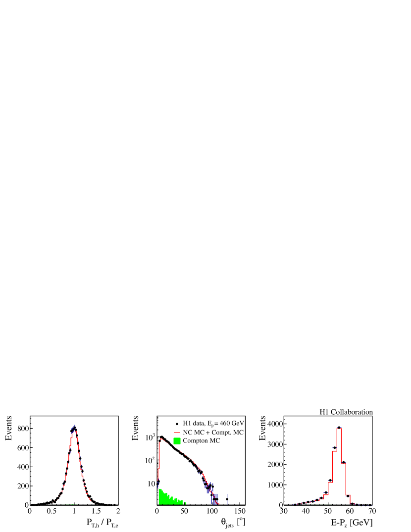
(a)

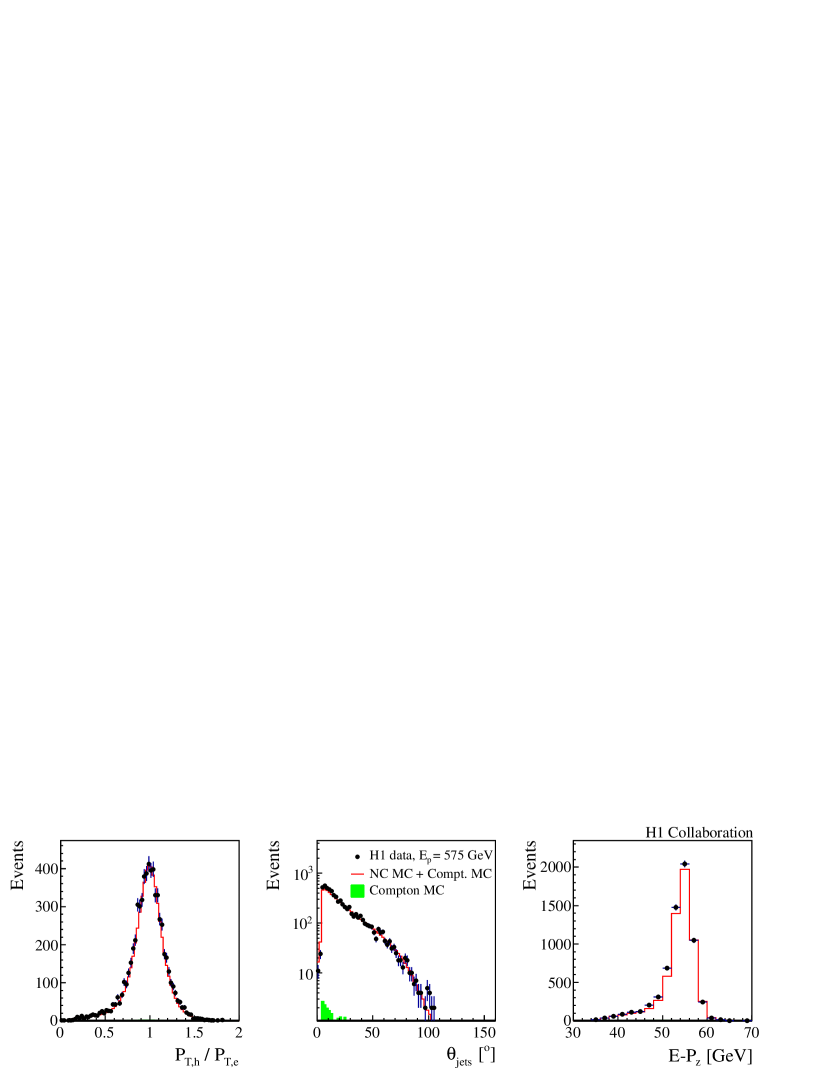
(b)

Figure 1: Distributions of $P_{\rm T,h}/P_{\rm T,e}$, $\theta_{\rm jets}$ and $E-P_{z}$ for (a) $E_{p}=460$ GeV and (b) $E_{p}=575$ GeV for $y<0.19$ data (solid points) and simulation and estimated background (histograms) normalised to the integrated luminosity of the data. The estimated QED Compton background contribution is shown as shaded histogram.

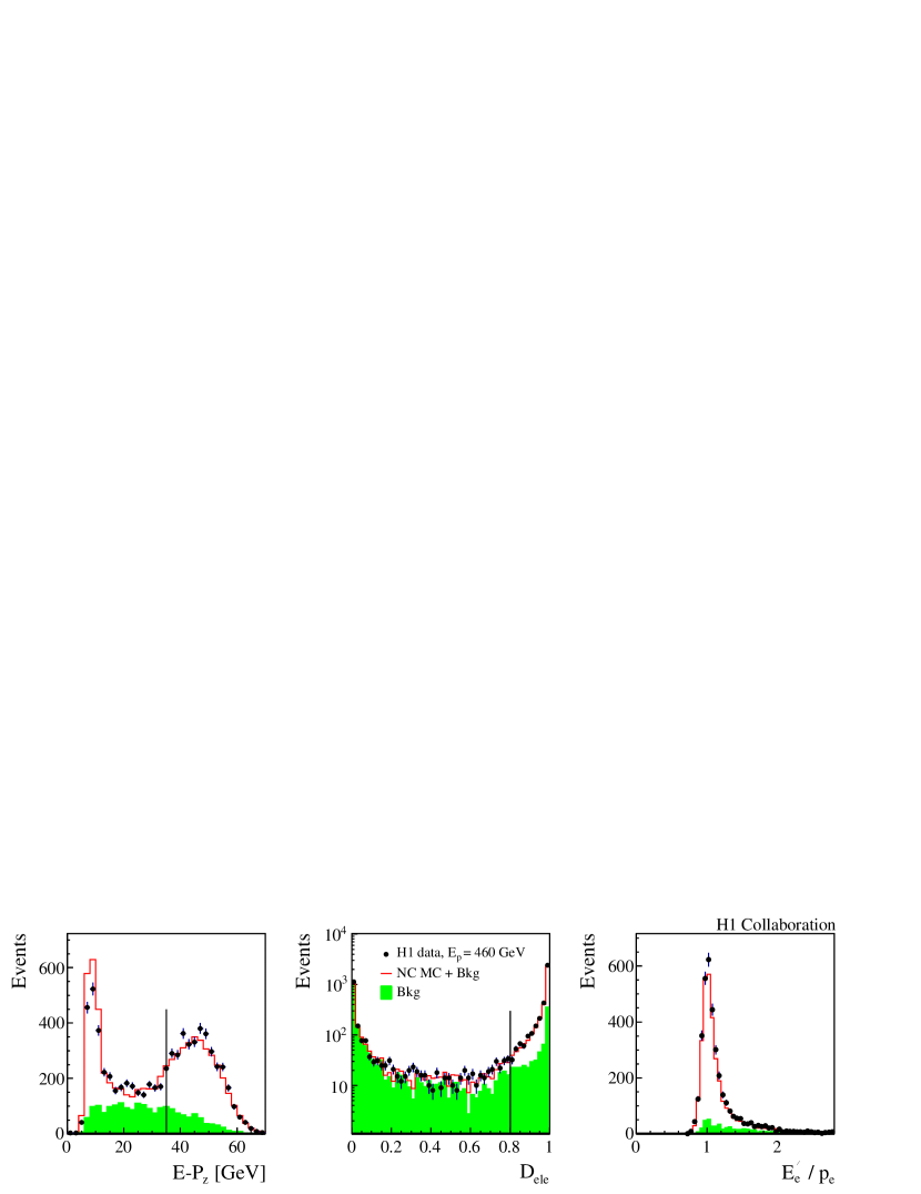
(a)

(b)

Figure 2: Distributions of $E-P_{z}$, $D_{ele}$, and $E^{\prime}_{e}/p_{e}$ for the sample of events with $E^{\prime}_{e}<6$ GeV. The selection requirements on $E-P_{z}$ and $D_{ele}$ are shown as vertical lines with all other selection criteria applied. The distributions are shown for (a) $E_{p}=460$ GeV and (b) $E_{p}=575$ GeV for data (solid points) and simulation and estimated background (histograms) normalised to the integrated luminosity of the data. The estimated background is shown as shaded histogram and includes the photoproduction contribution estimated using wrong charge scattered lepton candidates as well as the QED Compton contribution.

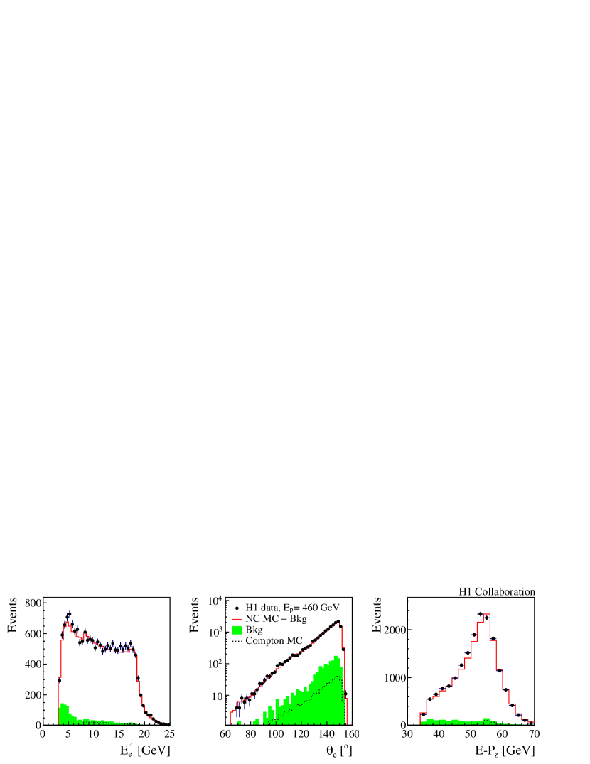
(a)

(b)

Figure 3: Distributions of $E^{\prime}_{e}$, $\theta_{e}$ and $E-P_{z}$ for (a) $E_{p}=460$ GeV and (b) $E_{p}=575$ GeV for $high~{}y$ data (solid points) and simulation and estimated background (histograms) normalised to the integrated luminosity of the data. The estimated background is shown as shaded histogram and includes the photoproduction contribution estimated using wrong charge scattered lepton candidates and the QED Compton contribution (dashed line).

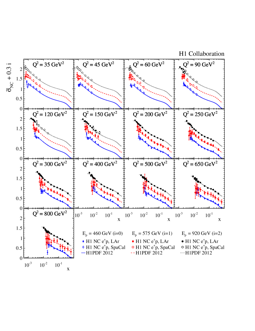
Figure 4: The reduced cross section $\tilde{\sigma}_{NC}(x,Q^{2})+0.3i$ measured at three proton beam energies $E_{p}=460$ GeV (diamonds, i=0), $575$ GeV (squares, i=1) and $920$ GeV (circles, i=2). The previously published H1 SpaCal data are shown by the open symbols. The solid symbols are the H1 LAr data. The new measurements reported here correspond to the filled diamonds and squares. The inner error bars represent the statistical errors, the full error bars include the statistical and systematic uncertainties added in quadrature, excluding the normalisation uncertainty. The curves represent the prediction from the H1PDF2012 NLO QCD fit.

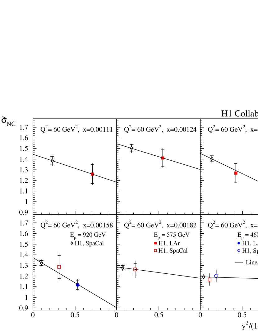
Figure 5: The reduced cross section $\tilde{\sigma}_{NC}(x,Q^{2})$ as a function of $y^{2}/(1+(1-y)^{2})$ for six values of $x$ at $Q^{2}=60$ GeV², measured for proton beam energies of $E_{p}=920,~{}575$ and $460$ GeV. The inner error bars denote the statistical error, the outer error bars show statistical and systematic uncertainties added in quadrature. The luminosity uncertainty is not included in the error bars. The negative slopes of the linear fits (solid line) which were performed using total errors, illustrate the non-vanishing values of the structure function $F_{L}(x,Q^{2})$.

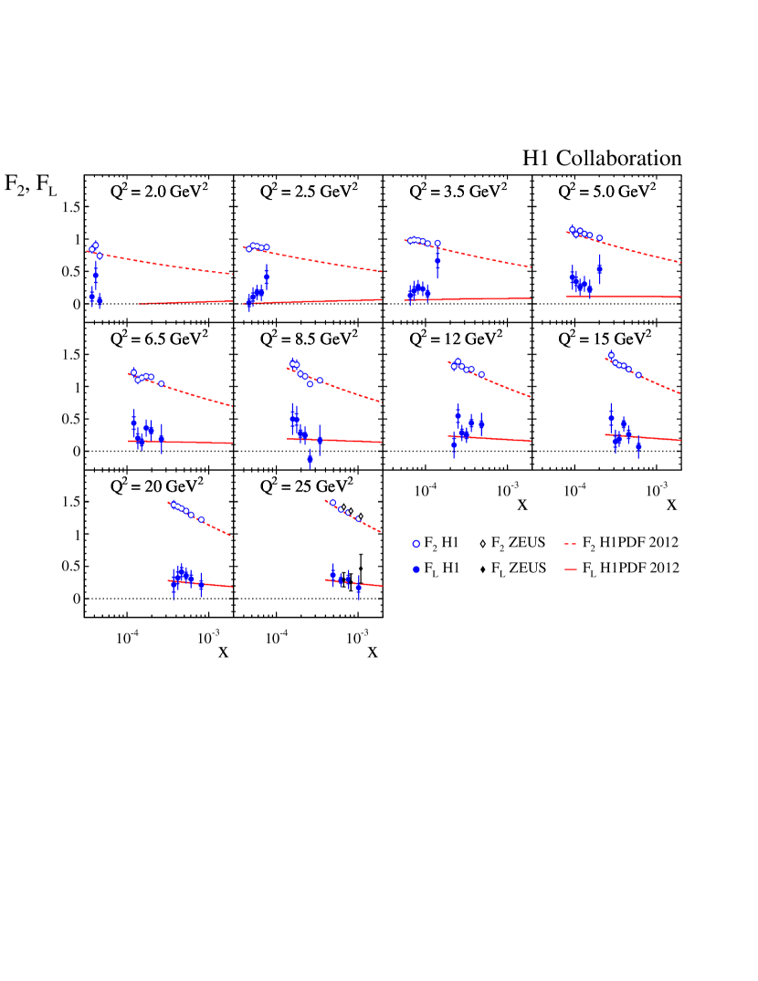
Figure 6: The proton structure functions $F_{L}(x,Q^{2})$ (solid symbols) and $F_{2}(x,Q^{2})$ (open symbols) measured by H1 (circles) and ZEUS (diamonds) in the region $2\leq Q^{2}\leq 25$ GeV². Only the $F_{2}(x,Q^{2})$ measurements obtained in the determinations of $F_{L}$ by H1 and ZEUS are shown. The inner error bars represent the statistical uncertainties, the full error bars include the statistical and systematic uncertainties added in quadrature, including all correlated and uncorrelated uncertainties. The curves represent the prediction from the H1PDF2012 NLO QCD fit.

Figure 7: The proton structure functions $F_{L}(x,Q^{2})$ (solid symbols) and $F_{2}(x,Q^{2})$ (open symbols) measured by H1 (circles) and ZEUS (diamonds) in the region $35\leq Q^{2}\leq 800$ GeV². Only the $F_{2}(x,Q^{2})$ measurements obtained in the determinations of $F_{L}$ by H1 and ZEUS are shown. The inner error bars represent the statistical uncertainties, the full error bars include the statistical and systematic uncertainties added in quadrature, including all correlated and uncorrelated uncertainties. The curves represent the prediction from the H1PDF2012 NLO QCD fit.

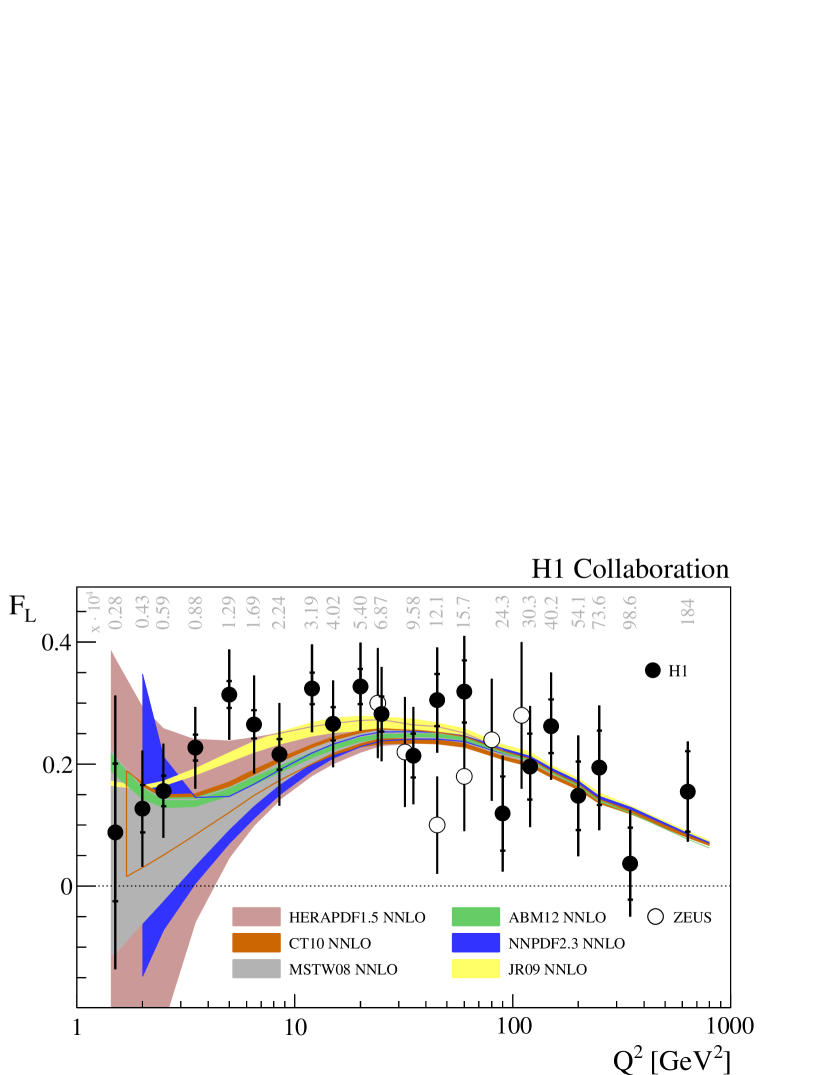
Figure 8: The proton structure function $F_{L}$ averaged over $x$ at different $Q^{2}$ (solid points). The average value of $x$ for each $Q^{2}$ is given above each data point. The inner error bars represent the statistical uncertainties, the full error bars include the statistical and systematic uncertainties added in quadrature, including all correlated and uncorrelated uncertainties. The $F_{L}$ measurements by ZEUS are also shown (open points). The data are compared to NNLO predictions from a selection of PDF sets as indicated.

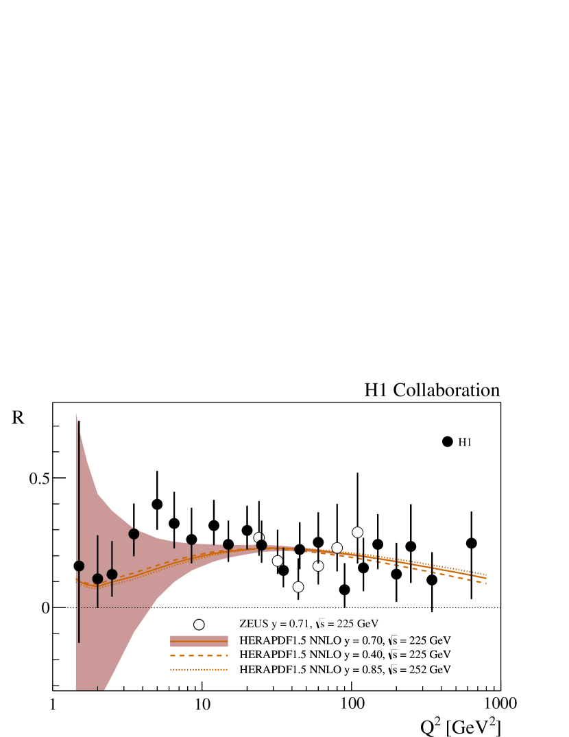
Figure 9: The ratio $R(Q^{2})$ averaged over $x$ in the region $1.5\leq Q^{2}\leq 800$ GeV² (solid points). The error bars represent the full errors as obtained by the Monte Carlo procedure described in the text. The ZEUS data are also shown (open symbols). The ZEUS data point at $Q^{2}=45$ GeV² is slightly shifted for better visibility of the erros. The solid curve represents the prediction from the HERAPDF1.5 NNLO QCD fit and its uncertainty for $\sqrt{s}=225$ Gev² and $y=0.7$. The additional dashed and dotted curves show the variations of $R$ in the region of $x$ where the data are sensitive to this quantity.

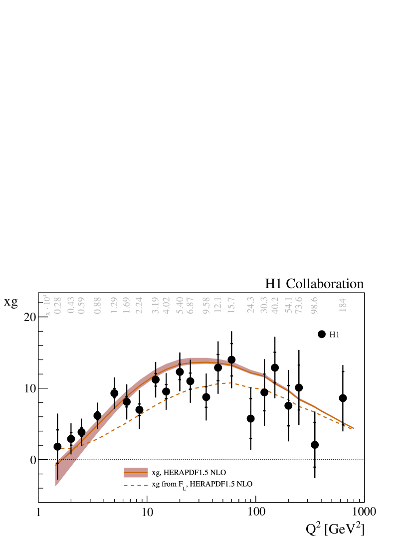
Figure 10: The gluon density $xg(x,Q^{2})$ averaged over $x$ in the region $1.5\leq Q^{2}\leq 800$ GeV² (solid points). The average value of $x$ for each $Q^{2}$ is given above each data point. The inner error bars represent the statistical uncertainties, the full error bars include the statistical and systematic uncertainties added in quadrature, including all correlated and uncorrelated uncertainties. The shaded regions represent the prediction from the HERAPDF1.5 NLO QCD fit. The dashed line corresponds to $xg$ as obtained by applying equation 8 to the $F_{L}$ prediction based on the HERAPDF1.5 NLO QCD fit.

References

- [1] E. Perez and E. Rizvi, Rep. Prog. Phys. 76 (2013) 046201 [arXiv:1208.1178].
- [2] F. D. Aaron et al. [H1 Collaboration], Phys. Lett. B665 (2008) 139 [arXiv:0805.2809].
- [3] F. D. Aaron et al. [ H1 Collaboration], Eur. Phys. J. C 71 (2011) 1579 [arXiv:1012.4355].
- [4] S. Chekanov et al. [ZEUS Collaboration], Phys. Lett. B 682 (2009) 8 [arXiv:0904.1092].
- [5] G. Altarelli and G. Martinelli, Phys. Lett. B76 (1978) 89.
- [6] F. D. Aaron et al. [H1 Collaboration], JHEP 1209 (2012) 061 [arXiv:1206.7007].
- [7] I. Abt et al. [H1 Collaboration], Nucl. Instrum. Meth. A386 (1997) 310.
- [8] I. Abt et al. [H1 Collaboration], Nucl. Instrum. Meth. A386 (1997) 348.
- [9] B. Andrieu et al. [H1 Calorimeter Group], Nucl. Instrum. Meth. A336 (1993) 460.
- [10] R. D. Appuhn et al. [H1 SPACAL Group], Nucl. Instrum. Meth. A386 (1997) 397.
- [11] B. Andrieu et al. [H1 Calorimeter Group], Nucl. Instrum. Meth. A336 (1993) 499.
- [12] B. Andrieu et al. [H1 Calorimeter Group], Nucl. Instrum. Meth. A350 (1994) 57.
- [13] J. Becker et al., Nucl. Instrum. Meth. A586 (2008) 190 [physics/0701002].
- [14] P. J. Laycock et al., The H1 forward track detector at HERA II, [arXiv:1206.4068].
- [15] D. Pitzl et al., Nucl. Instrum. Meth. A454 (2000) 334 [hep-ex/0002044].
- [16] B. List, Nucl. Instrum. Meth. A501 (2001) 49.
- [17] I. Glushkov, D* meson production in deep inelastic electron-proton scattering with the forward and backward silicon trackers of the H1 experiment at HERA, PhD thesis, Humboldt University, Berlin, 2008. Also available at http://www-h1.desy.de/publications/theses_list.html.
- [18] J. Kretzschmar, A precision measurement of the proton structure function with the H1 experiment, PhD thesis, Humboldt University, Berlin, 2008. Also available at http://www-h1.desy.de/publications/theses_list.html.
- [19] T. Nicholls et al., H1 SPACAL Group, Nucl. Instrum. Meth. A 374 (1996) 149.
- [20] A. A. Sokolov and I. M. Ternov, Sov. Phys. Dokl. 8 (1964) 1203.
- [21] M. Beckmann et al., Nucl. Instrum. Meth. A479 (2002) 334 [physics/0009047].
- [22] D. P. Barber et al., Nucl. Instrum. Meth. A338 (1994) 166.
- [23] B. Sobloher et al., Polarisation at HERA - Reanalysis of the HERA II Polarimeter Data, [arXiv:1201.2894]
-
[24]
A. Baird et al.,
IEEE Trans. Nucl. Sci. 48 (2001) 1276
[hep-ex/0104010];
D. Meer et al., IEEE Trans. Nucl. Sci. 49 (2002) 357 [hep-ex/0107010];
A. Schöning [H1 Collaboration], Nucl. Instrum. Meth. A 518 (2004) 542;
N. Berger et al., IEEE Nuclear Science Symposium Conf. Record, vol. 3, (2004) 1976;
A. Schöning [H1 Collaboration], Nucl. Instrum. Meth. A 566 (2006) 130. - [25] A.W. Jung et al., Proceedings of “15th IEEE-NPSS Real-Time Conference”, (2007).
- [26] B. Olivier et al., Nucl. Instrum. Meth. A 641 (2011) 58 [Erratum-ibid. A 724 (2013) 5].
- [27] F. D. Aaron et al. [H1 Collaboration], Eur. Phys. J. C 72 (2012) 2148 [arXiv:1206.4346].
- [28] M. Sauter, Measurement of Beauty Photoproduction at Threshold using Di-Electron Events with the H1 Detector at HERA, PhD thesis, DESY-THESIS-2009-047, ETH Zürich, Zürich, 2009. Also available at http://www-h1.desy.de/publications/theses_list.html.
- [29] F.D. Aaron et al. [H1Collaboration], Eur. Phys. J. C 72 (2012) 2163, Erratum-ibid. [arXiv:1205.2448].
- [30] G. A. Schuler and H. Spiesberger, DJANGO: The Interface for the event generators HERACLES and LEPTO, in Proceedings of the Workshop “Physics at HERA”, eds., W. Buchmüller and G. Ingelman, Hamburg, vol. 3, 1991, p. 1419.
- [31] A. Kwiatkowski, H. Spiesberger and H. J. Möhring, Comput. Phys. Commun. 69 (1992) 155.
- [32] G. Ingelman, LEPTO version 6.1: The Lund Monte Carlo for deep inelastic lepto - nucleon scattering, in Proceedings of the Workshop “Physics at HERA”, eds., W. Buchmüller and G. Ingelman, Hamburg, vol. 3, 1991, p. 1366.
- [33] L. Lönnblad, Comput. Phys .Commun. 71 (1992) 15.
- [34] T. Sjöstrand and M. Bengtsson, Comput. Phys. Commun. 43 (1987) 367.
- [35] S. Schael et al. [ALEPH Collaboration], Phys. Lett. B 606 (2005) 265.
- [36] V. Lendermann, H. C. Schultz-Coulon and D. Wegener, Eur. Phys. J. C 31 (2003) 343 [hep-ph/0307116].
- [37] R. Brun, F. Carminati and S. Giani, GEANT Detector Description and Simulation Tool, CERN Program Library Long Writeup W5013.
- [38] M. Peez, Search for Deviations from the Standard Model in High Transverse Energy Processes at the Electron Proton Collider HERA, PhD thesis, Lyon University, 2003; B. Portheault, First Measurement of Charged and Neutral Current Cross Sections with the Polarised Positron Beam at HERA II and QCD-Electroweak Analyses, PhD thesis, Paris XI ORSAY University, 2005; S. Hellwig, Untersuchung der Double Tagging Methode in Charmanalysen, Dipl. thesis, Hamburg University, 2004. Also available at http://www-h1.desy.de/publications/theses_list.html.
- [39] U. Bassler and G. Bernardi, Nucl. Instrum. Meth. A361 (1995) 197 [hep-ex/9412004].
- [40] U. Bassler and G. Bernardi, Nucl. Instrum. Meth. A426 (1999) 583 [hep-ex/9801017].
- [41] S. Catani, Y. L. Dokshitzer, M. H. Seymour and B. R. Webber, Nucl. Phys. B406 (1993) 187.
- [42] S. D. Ellis and D. E. Soper, Phys. Rev. D48 (1993) 3160 [hep-ph/9305266].
- [43] T. H. Tran, Precision measurement of cross sections of charged and neutral current processes at high at HERA, PhD thesis, Univ. Paris-Sud 11, 2010, DESY-THESIS-2011-009. Also available at http://www-h1.desy.de/publications/theses_list.html.
- [44] S. Bentvelsen et al., Proceedings of the Workshop “Physics at HERA”, eds., W. Buchmüller and G. Ingelman, Hamburg, vol. 1, 1991, p. 23
- [45] K. Hoeger,Proceedings of the Workshop “Physics at HERA”, eds., W. Buchmüller and G. Ingelman, Hamburg, vol. 1, 1991, p. 43.
- [46] R. Kogler, Measurement of jet production in deep-inelastic scattering at HERA, PhD thesis, Hamburg University, 2010, DESY-THESIS-2011-003, MPP-2010-175. Also available at http://www-h1.desy.de/publications/theses_list.html.
- [47] A. Nikiforov, Measurements of the neutral current cross sections using longitudinally polarised lepton beams at HERA II, PhD thesis, Ludwig-Maximilians-Univ., München, 2007. Also available at http://www-h1.desy.de/publications/theses_list.html.
- [48] S. Shushkevich, Measurement of neutral current cross sections with longitudinally polarised leptons at HERA, PhD thesis, MPP-2012-583, Ludwig-Maximilians-Univ., München, 2012. Also available at http://www-h1.desy.de/publications/theses_list.html.
- [49] M. Cacciari, G. P. Salam and G. Soyez, arXiv:1111.6097.
- [50] M. Cacciari and G. P. Salam, Phys. Lett. B641 (2006) 57 [hep-ph/0512210].
- [51] A. Hocker et al., PoS ACAT (2007) 040 [physics/0703039].
- [52] C. Adloff et al. [H1 Collaboration], Eur. Phys. J. C21 (2001) 33 [hep-ex/0012053].
- [53] F. D. Aaron et al. [H1 Collaboration], Eur. Phys. J. C71 (2010) 1579 [arXiv:1012.4355].
- [54] C. Adloff et al. [H1 Collaboration], Eur. Phys. J. C13 (2000) 609 [hep-ex/9908059].
- [55] C. Adloff et al. [H1 Collaboration], Eur. Phys. J. C30 (2003) 1 [hep-ex/0304003].
- [56] A. Arbuzov et al., Comput. Phys. Commun. 94 (1996) 128 [hep-ph/9511434].
- [57] H. Spiesberger, EPRC: A Program Package for electroweak Physics at HERA, in Proceedings of the Workshop “Future Physics at HERA”, eds., G. Ingelman, A. De Roeck and R. Klanner, Hamburg , vol. 1, 1995/6, p. 227.
- [58] S. Z. Habib, Unpolarized neutral current cross section measurements at the H1 experiment, HERA, PhD thesis, Hamburg University, 2009, DESY-THESIS-2009-039. Also available at http://www-h1.desy.de/publications/theses_list.html.
-
[59]
H1 and ZEUS Collaborations, preliminary result
http://www-h1.desy.de/publications/H1preliminary.short_list.html. - [60] H. -L. Lai et al., Phys. Rev. D 82 (2010) 074024 [arXiv:1007.2241].
- [61] S. Alekhin, J. Blüemlein and S. Moch, [arXiv:1310.3059].
- [62] A. D. Martin et al., Eur. Phys. J. C63 (2009) 189 [arXiv:0901.0002].
-
[63]
M. Gluck, P. Jimenez-Delgado and E. Reya,
Eur. Phys. J. C 53 (2008) 355
[arXiv:0709.0614];
P. Jimenez-Delgado and E. Reya, Phys. Rev. D 79 (2009) 074023 [arXiv:0810.4274]. -
[64]
R. D. Ball et al.,
Nucl. Phys. B 867 (2013) 244
[arXiv:1207.1303];
S. Forte et al., Nucl. Phys. B 834, 116 (2010) [arXiv:1001.2312]. - [65] F. James and M. Roos, Comput. Phys. Commun. 10 (1975) 343.
- [66] A. M. Cooper-Sarkar et al., Z. Phys. C 39 (1988) 281.
- [67] E. B. Zijlstra and W. L. van Neerven, Nucl. Phys. B 383 (1992) 525.
-
[68]
G. R. Boroun, B. Rezaei, Eur. Phys. J. C72 (2012) 2221;
G. R. Boroun, B. Rezaei, arXiv:1401.7804.