Array Convolutional Low-Density Parity-Check Codes

Abstract

This paper presents a design technique for obtaining regular time-invariant low-density parity-check convolutional (RTI-LDPCC) codes with low complexity and good performance. We start from previous approaches which unwrap a low-density parity-check (LDPC) block code into an RTI-LDPCC code, and we obtain a new method to design RTI-LDPCC codes with better performance and shorter constraint length. Differently from previous techniques, we start the design from an array LDPC block code. We show that, for codes with high rate, a performance gain and a reduction in the constraint length are achieved with respect to previous proposals. Additionally, an increase in the minimum distance is observed.

I Introduction

LDPC codes [1] are the state of the art in forward error correction, because of their capacity-achieving performance under belief propagation decoding [2]. These decoding algorithms work on the code Tanner graph, corresponding to the parity-check matrix $\mathbf{H}$, and have a complexity which increases linearly with the code length. Their best performance is achieved by using irregular codes, with degree distributions optimized through density evolution [3]. However, regular codes incur a loss with respect to irregular codes which decreases with increasing code rate, and becomes very small at high code rates, which are of interest in many practical applications. In addition, the code regularity simplifies the hardware implementation of the belief propagation decoder and allows a scalable design. Structured LDPC codes, like quasi-cyclic low-density parity-check (QC-LDPC) codes [4, 5] and low-density parity-check convolutional (LDPCC) codes [6, 7, 8] can also take advantage of simple encoding circuits.

In this paper, we focus on RTI-LDPCC codes. As for QC-LDPC codes, LDPCC codes can be encoded through simple circuits based on shift registers like that in [7, Fig. 4]. Their decoding can be performed by running a belief propagation algorithm on a window sliding over the received sequence [7]. Both these encoding and decoding methods have a complexity which increases linearly with the code syndrome former constraint length. Hence, we use the syndrome former constraint length as a measure of the complexity, and we aim at designing codes with small constraint lengths.

A well-known approach for designing time invariant LDPCC codes has been proposed by Tanner et al. in [6]. The codes designed in [6] are both regular and irregular and usually have large constraint lengths. Unfortunately, the RTI-LDPCC codes designed as in [6] often exhibit high error floors at high code rates. This was already observed in [9], where another class of RTI-LDPCC codes, named progressive difference convolutional low-density parity-check (PDC-LDPC) codes, was presented. Those codes have a known minimum distance and achieve strong reductions in the constraint length with respect to the approach in [6]. On the other hand, PDC-LDPC codes with high rate also exhibit rather high error floors, and do not outperform those designed following [6].

We propose a method to design RTI-LDPCC codes which represent a further step in this direction. In fact, the proposed codes, similarly to those in [9], achieve a smaller constraint length than their counterparts designed as in [6] but, contrary to [9], they are also able to achieve better performance at high code rates, which are of major interest for this kind of codes. Differently from previous solutions, the proposed design starts from a special class of QC-LDPC codes, named array LDPC codes [10]. For this reason, we call these codes array convolutional low-density parity-check (AC-LDPC) codes. The organization of the paper is as follows: in Section II, we remind the main characteristics of array LDPC codes; in Section III, we define the new class of AC-LDPC codes; in Section IV, we compare this approach with previously proposed solutions; in Section V, we provide some design examples and conclusive remarks.

II Array LDPC codes

Array LDPC codes are a special class of QC-LDPC codes. A quasi-cyclic (QC) code has dimension $k$ and length $n$ which are both multiple of a positive integer $q$, i.e., $k=k_{0}q$ and $n=n_{0}q$. Hence, the code redundancy is $r=(n_{0}-k_{0})q=r_{0}q$. In a QC code, every cyclic shift of $n_{0}$ positions of a codeword yields another codeword. When a QC code is also an LDPC code, it is called a QC-LDPC code. The parity-check matrix $\mathbf{H}$ of a QC code has the following form:

$$\mathbf{H}=\left[\begin{array}[]{llll}\mathbf{H}_{0,0}^{c}&\mathbf{H}_{0,1}^{c}&\ldots&\mathbf{H}_{0,n_{0}-1}^{c}\\ \mathbf{H}_{1,0}^{c}&\mathbf{H}_{1,1}^{c}&\ldots&\mathbf{H}_{1,n_{0}-1}^{c}\\ \vdots&\vdots&\ddots&\vdots\\ \mathbf{H}_{r_{0}-1,0}^{c}&\mathbf{H}_{r_{0}-1,1}^{c}&\ldots&\mathbf{H}_{r_{0}-1,n_{0}-1}^{c}\end{array}\right].$$ (1)

In (1), each $\mathbf{H}_{i,j}^{c}$ is a $q\times q$ circulant matrix, i.e., a square matrix whose $l$-th row, $l=0,1,2,\ldots,q-1$, is obtained by a right cyclic shift of the first row by $l$ positions.

For QC-LDPC codes, each matrix $\mathbf{H}_{i,j}^{c}$ is a sparse circulant matrix or a null matrix, and $\mathbf{H}$ is free of short cycles in its associated Tanner graph. A special family of QC-LDPC codes is obtained by using circulant permutation matrices as $\mathbf{H}_{i,j}^{c}$ [11]. In this case, each circulant permutation matrix is represented as a power of the unitary circulant permutation matrix $\mathbf{P}$. The identity matrix is $\mathbf{P}^{0}$. For this kind of QC-LDPC codes, choosing a prime $q$ ensures some desirable properties [11]. Array LDPC codes are based on circulant permutation matrices, and require a prime $q$. Also the codes used in [6] are based on circulant permutation matrices and often use a prime $q$ (although it is not mandatory). Hence, from now on we consider only prime values of $q$. Let $\mathbf{\Delta}=\{\Delta_{0},\Delta_{1},\Delta_{2},\ldots,\Delta_{r_{0}-1}\}$ be a set of $r_{0}$ distinct integers, with $\Delta_{0}<\Delta_{1}<\Delta_{2}<\cdots<\Delta_{r_{0}-1}<q$, $0<r_{0}<n_{0}\leq q$, and let us define

$$\mathbf{H}_{a}=\begin{bmatrix}{0}&{\Delta_{0}}&{2\Delta_{0}}&\ldots&{(n_{0}-1)\Delta_{0}}\\ {0}&{\Delta_{1}}&{2\Delta_{1}}&\ldots&{(n_{0}-1)\Delta_{1}}\\ {0}&{\Delta_{2}}&{2\Delta_{2}}&\ldots&{(n_{0}-1)\Delta_{2}}\\ \vdots&\vdots&\vdots&\ddots&\vdots\\ {0}&{\Delta_{r_{0}-1}}&{2\Delta_{r_{0}-1}}&\ldots&{(n_{0}-1)\Delta_{r_{0}-1}}\end{bmatrix}.$$ (2)

An array LDPC code is defined by the parity-check matrix $\mathbf{H}$ which is obtained by using the elements of $\mathbf{H}_{a}$ as the exponents of $\mathbf{P}$. Due to the primality of $q$, $\mathbf{H}$ is free of length-$4$ cycles. If $n_{0}=q$, we have a full length array LDPC code. In fact, for $n_{0}>q$, the code becomes trivial, and its minimum distance drops to $2$. Choosing $n_{0}<q$ instead produces a shortened array LDPC code. Reordering the columns of $\mathbf{H}$ yields an equivalent code. Reordering is usually performed by moving blocks of $q$ columns each, such that the QC form of $\mathbf{H}$ is preserved. Shortening can also be performed after having reordered the columns of $\mathbf{H}$, thus obtaining a code which is not necessarily equivalent to the non-reordered shortened array code. Another classification of array codes depends on the choice of $\mathbf{\Delta}$: if $\mathbf{\Delta}=\{0,1,2,\ldots,{r_{0}-1}\}$, the code is called a proper array LDPC code, otherwise it is an improper array LDPC code.

Theoretical arguments can be used to predict the minimum distance of array LDPC codes, or to find bounds on it. The minimum distance of proper full length array LDPC codes can be upper bounded by using the approach proposed in [12, 13], which also simplifies the search of low weight codewords. The minimum distance of proper full length array LDPC codes can be improved by resorting to improper [14] and shortened codes [15], thus approaching the values achievable through other design techniques based on circulant permutation matrices. A general form for the generator matrix of array LDPC codes has been presented in [16], and helps deriving general upper bounds on their minimum distance.

III Array Convolutional LDPC codes

Starting from the parity-check matrix $\mathbf{H}$ of an array LDPC code, we aim at obtaining an unwrapped version of it, to form the semi-infinite binary parity-check matrix $\mathbf{H}_{\mathrm{conv}}$ of an RTI-LDPCC code. For this purpose, let us rearrange the rows and the columns of $\mathbf{H}$ as follows: permute the rows according to the ordering $0,q,2q,\ldots,(r_{0}-1)q,1,q+1,2q+1,\ldots,(r_{0}-1)q+1,\ldots,q-1,2q-1,3q-1,\ldots,r_{0}q-1$ and then permute the columns according to the ordering $0,q,2q,\ldots,(n_{0}-1)q,1,q+1,2q+1,\ldots,(n_{0}-1)q+1,\ldots,q-1,2q-1,3q-1,\ldots,n_{0}q-1$. This way, we swap the inner and outer structures of the original matrix, which is a block of circulants, and obtain the parity-check matrix of an equivalent code in the form of a circulant of blocks, that is

$$\mathbf{H}=\left[\begin{array}[]{llll}\mathbf{H}_{0}&\mathbf{H}_{1}&\ldots&\mathbf{H}_{q-1}\\ \mathbf{H}_{q-1}&\mathbf{H}_{0}&\ldots&\mathbf{H}_{q-2}\\ \vdots&\vdots&\ddots&\vdots\\ \mathbf{H}_{1}&\mathbf{H}_{2}&\ldots&\mathbf{H}_{0}\end{array}\right],$$ (3)

where each block $\mathbf{H}_{i}$ is of size $r_{0}\times n_{0}$. Starting from $\mathbf{H}$ in (3), we apply the unwrapping method in [7]. However, differently from [7], where time-varying convolutional codes are designed, we obtain time-invariant codes. In fact, using the unwrapping in [7] with a cutting pattern such that we repeatedly move $n_{0}$ positions to the right and then $r_{0}$ positions down, we obtain the following semi-infinite parity-check matrix:

$$\mathbf{H}_{\mathrm{conv}}=\left[\begin{array}[]{cccccc}\mathbf{H}_{0}&\mathbf{0}&\mathbf{0}&\cdots\\ \mathbf{H}_{q-1}&\mathbf{H}_{0}&\mathbf{0}&\cdots\\ \mathbf{H}_{q-2}&\mathbf{H}_{q-1}&\mathbf{H}_{0}&\cdots\\ \vdots&\vdots&\vdots&\ddots\\ \mathbf{H}_{1}&\mathbf{H}_{2}&\mathbf{H}_{3}&\ddots\\ \mathbf{0}&\mathbf{H}_{1}&\mathbf{H}_{2}&\ddots\\ \mathbf{0}&\mathbf{0}&\mathbf{H}_{1}&\ddots\\ \mathbf{0}&\mathbf{0}&\mathbf{0}&\ddots\\ \vdots&\vdots&\vdots&\ddots\\ \end{array}\right],$$ (4)

which defines a time-invariant convolutional code with syndrome former matrix $\mathbf{H}_{s}=\left[\mathbf{H}_{0}^{T}|\mathbf{H}_{q-1}^{T}|\mathbf{H}_{q-2}^{T}|\ldots|\mathbf{H}_{1}^{T}\right]$, where ^T denotes transposition. We say that this code is regular since $\mathbf{H}_{s}$ is regular. Actually, the code defined by $\mathbf{H}_{\mathrm{conv}}$ is column-wise regular and only asymptotically row-wise regular, due to the effect of termination, which however is negligible for long block lengths and sliding-window decoding. We have:

• Asymptotic code rate: $R=k_{0}/n_{0}$.

• Parity-check matrix column weight: $r_{0}$.

• Syndrome former memory order: $m_{s}=q$.

• Syndrome former constraint length: $v_{s}=q\cdot n_{0}$.

IV Comparison with previous solutions

An LDPCC code is often obtained by designing an LDPC block code and then unwrapping it. Two main methods exist for this purpose: the former starts from a specific class of QC-LDPC block codes to obtain time-invariant LDPCC codes [6], whereas the latter starts from generic LDPC block codes to obtain time-varying LDPCC codes [7].

The method we propose, described in Section III, can be seen as a variant of them both, with the main difference of using another class of QC-LDPC block codes as the starting point. In general, the codes designed according to [7] are time-varying, while we obtain time invariant codes by using array LDPC codes as our starting point. Concerning the method in [6], its starting point is instead a QC-LDPC block code obtained from the following exponent matrix:

$$\mathbf{H}_{a}^{[6]}=\begin{bmatrix}1&a&a^{2}&\ldots&a^{n_{0}-1}\\ b&ab&a^{2}b&\ldots&a^{n_{0}-1}b\\ b^{2}&ab^{2}&a^{2}b^{2}&\ldots&a^{n_{0}-1}b^{2}\\ \vdots&\vdots&\vdots&\vdots&\ddots\\ b^{r_{0}-1}&ab^{r_{0}-1}&a^{2}b^{r_{0}-1}&\ldots&a^{n_{0}-1}b^{r_{0}-1}\end{bmatrix}$$ (5)

where $a$ and $b$ are two integers with multiplicative orders equal to $n_{0}$ and $r_{0}$ modulo $m$, respectively, and $m$ is an integer $>r_{0}\cdot n_{0}$, such that $r_{0}$ and $n_{0}$ divide $m-1$. Choosing the smallest $m$ with these characteristics allows to minimize the constraint length. The elements of $\mathbf{H}_{a}^{[6]}$ (which are modulo $m$) are used as the exponents of the unitary circulant permutation matrix $\mathbf{P}$ of size $q=m$ to create the parity-check matrix of a QC-LDPC block code. An RTI-LDPCC code is obtained from the QC-LDPC block code through the unwrapping procedure described in [6]. The memory order of the resulting code equals the maximum value taken by the difference between the largest and the smallest elements in each row of $\mathbf{H}_{a}^{[6]}$, increased by one [8]. As acknowledged in [6], these LDPCC codes typically have large constraint lengths.

We observe that the exponent matrix (5) defines the same code that can be obtained by starting from an array LDPC code with $\mathbf{\Delta}=\{1,b,b^{2},\ldots,b^{r_{0}-1}\}$, and then performing column reordering, followed by shortening. So, the codes used as the starting point in [6] are a special case of array LDPC codes. Inspired by this observation, we use more general array LDPC codes than those obtained from (5) as our starting point to design RTI-LDPCC codes. After fixing $\mathbf{\Delta}$, we use the matrix (2) as the starting point of the unwrapping procedure, and this allows to obtain unwrapped codes with smaller constraint length than when starting from the matrix (5), as in [6]. In addition, at high code rates, the performance of the unwrapped codes and, in some cases, their minimum distance are improved, as we will show in Section V. Moreover, this allows to find a tradeoff between the constraint length and the performance by varying $q$, as we will also show next.

Concerning the unwrapping method, we use the one described in Section III, which exploits the technique proposed in [7]. Alternatively, we could replace the matrix (5) with (2) and use again the unwrapping method in [6]. This would produce similar results, as we will show in Example IV.1. We prefer to use the procedure in Section III because it makes easier to outline the structure of the syndrome former matrix $\mathbf{H}_{s}$.

Example IV.1

In order to provide an explicit simple example of the proposed method, let us consider the following two exponent matrices defining, respectively, a full length proper array LDPC code with $r_{0}=3,n_{0}=q=5$ and a shortened proper array LDPC code with $r_{0}=3,n_{0}=5,q=7$:

$$\mathbf{H}^{\prime}_{a}=\begin{bmatrix}0&0&0&0&0\\ 0&1&2&3&4\\ 0&2&4&1&3\end{bmatrix},\ \ \mathbf{H}^{\prime\prime}_{a}=\begin{bmatrix}0&0&0&0&0\\ 0&1&2&3&4\\ 0&2&4&6&1\end{bmatrix}.$$ (6)

We can unwrap them to obtain two RTI-LDPCC codes with rate $2/5$. By using the method in Section III, we get two AC-LDPC codes having the syndrome former matrices reported in Figs. 1 (a) and (c), respectively. These two LDPCC codes have $(m_{s},v_{s})$ equal to $(5,25)$ and $(7,35)$. If we instead follow the approach in [6], starting from the matrix (5), we are forced to accept longer constraint lengths. An LDPCC code with the same parameters (see [6, Example 6]) would have $(m_{s}=22,v_{s}=105)$. Finally, we observe that, by using the unwrapping technique in [6], but starting from $\mathbf{H}^{\prime}_{a}$ and $\mathbf{H}^{\prime\prime}_{a}$ in (6), we obtain the syndrome former matrices reported in Figs. 1 (b) and (d). As anticipated, these are very similar to those obtained through the alternative unwrapping technique we consider, since they are row-reordered versions of them.

$\scriptsize\begin{bmatrix}1&1&1&1&1\\ 1&0&0&0&0\\ 1&0&0&0&0\\ 0&0&0&0&0\\ 0&0&0&0&1\\ 0&0&1&0&0\\ 0&0&0&0&0\\ 0&0&0&1&0\\ 0&0&0&0&1\\ 0&0&0&0&0\\ 0&0&1&0&0\\ 0&1&0&0&0\\ 0&0&0&0&0\\ 0&1&0&0&0\\ 0&0&0&1&0\end{bmatrix}$

(a)

$\scriptsize\begin{bmatrix}0&0&1&0&0\\ 0&0&0&0&1\\ 0&0&0&0&0\\ 0&0&0&0&1\\ 0&0&0&1&0\\ 0&0&0&0&0\\ 0&1&0&0&0\\ 0&0&1&0&0\\ 0&0&0&0&0\\ 0&0&0&1&0\\ 0&1&0&0&0\\ 0&0&0&0&0\\ 1&0&0&0&0\\ 1&0&0&0&0\\ 1&1&1&1&1\end{bmatrix}$

(b)

$\scriptsize\begin{bmatrix}1&1&1&1&1\\ 1&0&0&0&0\\ 1&0&0&0&0\\ 0&0&0&0&0\\ 0&0&0&0&0\\ 0&0&0&1&0\\ 0&0&0&0&0\\ 0&0&0&0&0\\ 0&0&0&0&0\\ 0&0&0&0&0\\ 0&0&0&0&1\\ 0&0&1&0&0\\ 0&0&0&0&0\\ 0&0&0&1&0\\ 0&0&0&0&0\\ 0&0&0&0&0\\ 0&0&1&0&0\\ 0&1&0&0&0\\ 0&0&0&0&0\\ 0&1&0&0&0\\ 0&0&0&0&1\end{bmatrix}$

(c)

$\scriptsize\begin{bmatrix}0&0&0&1&0\\ 0&0&0&0&0\\ 0&0&0&0&0\\ 0&0&0&0&0\\ 0&0&0&0&0\\ 0&0&0&0&0\\ 0&0&1&0&0\\ 0&0&0&0&1\\ 0&0&0&0&0\\ 0&0&0&0&0\\ 0&0&0&1&0\\ 0&0&0&0&0\\ 0&1&0&0&0\\ 0&0&1&0&0\\ 0&0&0&0&0\\ 0&0&0&0&1\\ 0&1&0&0&0\\ 0&0&0&0&0\\ 1&0&0&0&0\\ 1&0&0&0&0\\ 1&1&1&1&1\end{bmatrix}$

(d)

Figure 1: Syndrome former matrices of LDPC convolutional codes obtained from the codes defined by $\mathbf{H}^{\prime}_{a}$ (a), (b) and $\mathbf{H}^{\prime\prime}_{a}$ (c), (d) in (6), through the use of the unwrapping technique in Section III (a), (c) and that in [6] (b), (d).

Another benchmark for the proposed class of codes are PDC-LDPC codes [9]. They are characterized by a very small syndrome former constraint length, and may have fixed minimum distance, independently of the code rate. However, the very small constraint length of PDC-LDPC codes is paid in terms of performance, which barely approaches that of the codes designed following [6]. As we will show in Section V, the newly proposed AC-LDPC codes instead allow to trade the syndrome former constraint length for performance, thus outperforming both these previous approaches.

V Performance assessment

We consider some code examples and simulate coded transmissions over the additive white Gaussian noise channel, with binary phase shift keying. LDPC decoding is performed through the sum-product algorithm with log-likelihood ratios, with $100$ maximum iterations, working over blocks of $60000$ bits. These choices ensure that the decoding algorithm achieves optimal performance for all the considered codes.

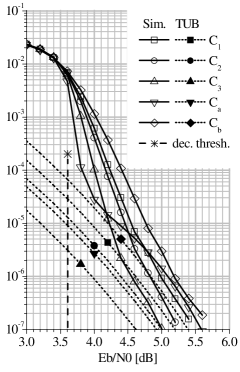
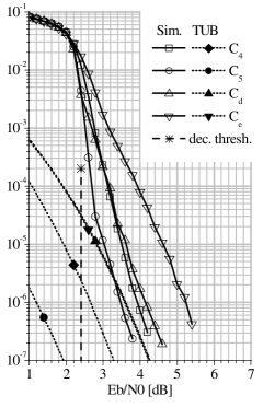
The code parameters are summarized in Tables I and II, where $R$ denotes the code rate, $w$ is the parity-check matrix column weight and $d$ the minimum distance. The latter has been estimated through Montecarlo simulations, by isolating the unique error vectors generating the low weight codewords observed. This way, as done in [17], we have estimated the spectrum of the lowest weights for each code, and this has been used to compute the corresponding truncated union bound (TUB) [18]. Table I reports the details of the shortened proper and improper AC-LDPC codes we have designed, whereas Table II provides the parameters of the other codes we have used as a benchmark, designed according to [6] and [9]. The weight spectra are not reported for the lack of space. For improper AC-LDPC codes, $\mathbf{\Delta}$ has been optimized heuristically. Fig. 2 shows the bit error rate (BER) and TUB curves for all codes, grouped by code rate. The decoding thresholds obtained through density evolution are also plotted.

TABLE I: Examples of AC-LDPC codes

Code	$R$	$r_{0}$	$n_{0}$	$w$	$\mathbf{\Delta}$	$q$	$v_{s}$	$d$
$C_{1}$	$0.9$	$3$	$30$	$3$	$\{0,1,2\}$	$43$	$1290$	$6$
$C_{2}$	$0.9$	$3$	$30$	$3$	$\{0,11,37\}$	$43$	$1290$	$6$
$C_{3}$	$0.9$	$3$	$30$	$3$	$\{0,11,37\}$	$71$	$2130$	$6$
$C_{4}$	$0.75$	$4$	$16$	$4$	$\{0,1,2,3\}$	$71$	$1136$	$10$
$C_{5}$	$0.75$	$4$	$16$	$4$	$\{0,11,37,70\}$	$71$	$1136$	$12$

TABLE II: Examples of other regular time invariant LDPC convolutional codes

Code	$R$	$r_{0}$	$n_{0}$	$w$	$\{m,a,b\}$	$v_{s}$	$d$
$C_{a}$ [6]	$0.9$	$3$	$30$	$3$	$\{151,23,32\}$	$4500$	$6$
$C_{b}$ [9]	$0.9$	$1$	$10$	$3$	$-$	$400$	$6$
$C_{d}$ [6]	$0.75$	$4$	$16$	$4$	$\{97,8,22\}$	$1536$	$8$
$C_{e}$ [9]	$0.75$	$1$	$4$	$4$	$-$	$152$	$8$

From the tables we observe that all the codes with rate $0.9$ have minimum distance $6$. However, the code $C_{3}$ has the lowest multiplicity of minimum weight codewords, which reflects into a better TUB. This is also confirmed by the simulation curves, since $C_{3}$ achieves a gain of $0.6$ dB or more over $C_{a}$ and $C_{b}$. In addition, it has a constraint length $v_{s}$ more than halved than that of $C_{a}$. The codes $C_{1}$ and $C_{2}$ achieve a further reduction in the constraint length, but at the cost of some loss in performance. The benefits of the proposed design technique are even more evident for codes with rate $0.75$, at which AC-LDPC codes also achieve higher minimum distances than those designed according to [6] and [9]. In fact, $C_{4}$ and $C_{5}$ have better BER and TUB curves than $C_{d}$ and $C_{e}$, and also achieve a reduction in the constraint length with respect to $C_{d}$. The code $C_{e}$ has the worst performance, but its constraint length is largely below that of all the other codes. As expected, these codes incur some performance loss with respect to irregular time-varying LDPCC codes with optimized degree distributions. For example, the rate $3/4$ code reported in [8, Fig. 9] exhibits a gain of about $0.8$ dB over $C_{5}$. However, it has a constraint length more than doubled, and requires to deal with an irregular and time-varying structure.

(a)

(b)

Figure 2: Simulated BER and TUB curves and decoding thresholds for the codes in Tables I and II with (a) rate $0.9$ and (b) rate $0.75$.

References

- [1] R. G. Gallager, “Low-density parity-check codes,” IRE Trans. Inform. Theory, vol. IT-8, pp. 21–28, Jan. 1962.
- [2] T. Richardson and R. Urbanke, “The capacity of low-density parity-check codes under message-passing decoding,” IEEE Trans. Inform. Theory, vol. 47, no. 2, pp. 599–618, Feb. 2001.
- [3] S.-Y. Chung, T. J. Richardson, and R. L. Urbanke, “Analysis of sum-product decoding of low-density parity-check codes using a gaussian approximation,” IEEE Trans. Inform. Theory, vol. 47, no. 2, pp. 657–670, Feb. 2001.
- [4] S. Lin and D. J. Costello, Error Control Coding, 2nd ed. Upper Saddle River, NJ: Prentice-Hall, Inc., 2004.
- [5] M. Baldi, F. Bambozzi, and F. Chiaraluce, “On a family of circulant matrices for quasi-cyclic low-density generator matrix codes,” IEEE Trans. Inform. Theory, vol. 57, no. 9, pp. 6052–6067, Sep. 2011.
- [6] R. M. Tanner, D. Sridhara, A. Sridharan, T. E. Fuja, and D. J. Costello, “LDPC block and convolutional codes based on circulant matrices,” IEEE Trans. Inform. Theory, vol. 50, no. 12, pp. 2966–2984, Dec. 2004.
- [7] A. Jimènez Felström and K. S. Zigangirov, “Time-varying periodic convolutional codes with low-density parity-check matrix,” IEEE Trans. Inform. Theory, vol. 45, no. 6, pp. 2181–2191, Sep. 1999.
- [8] A. E. Pusane, R. Smarandache, P. O. Vontobel, and D. J. Costello, “Deriving good LDPC convolutional codes from LDPC block codes,” IEEE Trans. Inform. Theory, vol. 57, no. 2, pp. 835–857, Feb. 2011.
- [9] M. Baldi, M. Bianchi, G. Cancellieri, and F. Chiaraluce, “Progressive differences convolutional low-density parity-check codes,” IEEE Commun. Lett., vol. 16, no. 11, pp. 1848–1851, Nov. 2012.
- [10] J. L. Fan, “Array codes as low-density parity-check codes,” in Proc. 2nd Int. Symp. Turbo Codes, Brest, France, Sep. 2000, pp. 543–546.
- [11] M. P. C. Fossorier, “Quasi-cyclic low-density parity-check codes from circulant permutation matrices,” IEEE Trans. Inform. Theory, vol. 50, no. 8, pp. 1788–1793, Aug. 2004.
- [12] K. Yang and T. Helleseth, “On the minimum distance of array codes as LDPC codes,” IEEE Trans. Inform. Theory, vol. 49, no. 12, pp. 3268–3271, Dec. 2003.
- [13] K. Sugiyama and Y. Kaji, “On the minimum weight of simple full length array LDPC codes,” IEICE Trans. on Fundamentals, vol. E91-A, no. 6, pp. 1502–1508, Jun. 2008.
- [14] M. Esmaeili, M. H. Tadayon, and T. A. Gulliver, “More on the stopping and minimum distances of array codes,” IEEE Trans. Commun., vol. 59, no. 3, pp. 750–757, Mar. 2011.
- [15] O. Milenkovic, N. Kashyap, and D. Leyba, “Shortened array codes of large girth,” IEEE Trans. Inform. Theory, vol. 52, no. 8, pp. 3707–3722, Aug. 2006.
- [16] M. Baldi, M. Bianchi, G. Cancellieri, F. Chiaraluce, and T. Kløve, “On the generator matrix of array LDPC codes,” in Proc. SoftCOM 2012, Split, Croatia, Sep. 2012.
- [17] C. Snow, L. Lampe, and R. Schober, “Error rate analysis for coded multicarrier systems over quasi-static fading channels,” IEEE Trans. Commun., vol. 55, no. 9, pp. 1736–1746, Sep. 2007.
- [18] G. Poltyrev, “Bounds on the decoding error probability of binary linear codes via their spectra,” IEEE Trans. Inform. Theory, vol. 40, no. 4, pp. 1284–1292, Jul. 1994.