Multiscaling edge effects in an agent-based money emergence model
Abstract
An agent-based computational economical toy model for the emergence of money from the initial barter trading, inspired by Menger’s postulate that money can spontaneously emerge in a commodity exchange economy, is extensively studied. The model considered, while manageable, is significantly complex, however. It is already able to reveal phenomena that can be interpreted as emergence and collapse of money as well as the related competition effects. In particular, it is shown that - as an extra emerging effect - the money lifetimes near the critical threshold value develop multiscaling, which allow one to set parallels to critical phenomena and, thus, to the real financial markets.
89.65.Gh, 05.45.Df, 05.70.Jk
1 Introduction
Extreme complexity of a phenomenon commonly termed as money stems from several factors. Viewed in contemporary terms as a foreign exchange (Forex) market it can be considered the world’s largest and most important financial market, entirely decentralized, crossing all the countries, with the highest daily trading volume extending to trillions of US dollars. There is plenty of evidence [1] that the Forex’s dynamics is more complex than that of any other market’s. The absence of an independent reference frame makes the absolute currency pricing virtually impossible and a given currency’s value is expressed by means of some other currency, which, in turn, is also denominated only in currencies. Moreover, in global terms the Forex market is exposed to current situation on other markets in all parts of the world, which makes it particularly sensitive and unpredictable. These facts together with other Forex specific relationships like the triangle rule [2, 3] that links mutual exchange rates of three currencies are among the factors responsible for a highly convoluted structure [4, 5, 6] of Forex.
Complexity of money as a general medium of exchange that allows to avoid difficulties of barter trade requiring a ”double coincidence of needs” and constitutes a measure of and a store of value, roots back even to its beginnings. Menger [7] proposed that money can spontaneously emerge in a commodity exchange economy. Accordingly, each commodity is characterized by its own marketability reflecting its status in the market. Money is a commodity, which through the process analogous to the physical spontaneous symmetry breaking [8] receives a very high marketability and thus a special status of a medium of exchange [9]. Katsuhito [10, 11] developed a model along the original Menger’s idea and demonstrated that money is governed by a kind of the so-called bootstrap mechanism, i.e., it is accepted at any place at any time because it is in a position of money. Agent based variants of such a model have further been studied by Yasutomi [12, 13] and Górski et al. [14] who by numerical simulations demonstrated that they are able to reveal money emergence as well as its collapse. In general, agent based models [15, 16] find an increasing number of promising applications in various areas of economics [12, 17, 18, 19, 20, 21] and in social sciences [22, 23, 24, 25, 26] and the need for this kind of approaching the related phenomena, especially in an economic context, is being expressed more and more forcefully [27, 28, 29]. For all these reasons in the present contribution, we further pursue simulations based on an agent based model which from an initial barter trading is able to spontaneously elevate one of the commodities to the money status. We in particular focus on the transition region between the homogenous commodities and emerging money phases with the aim to identify the complexity characteristics of this transition in terms of the multifractal scaling. Below we list the main ingredients of the model used.
2 Model
In the model [12, 14] we have agents, each agent producing one type of good enumerated by . For the sake of simplicity, we assume that the agent number is producing a good type denoted by . The elementary interaction of two agents (”transaction”) consist of several steps including search of the co-trader, exchange of particular goods, change of the agent’s buying preferences and finally the production and consumption phase. A sequence of consecutive transactions is called a turn. In a single turn each of the agents has chance to take part in exchange of goods, production, and consumption. To each agent, say , there are attributed three -dimensional vectors. The possession vector, , , with non-negative integer components that denote how many units of the -th good has the th agent at the moment. The demand vector, , is actually a ”shopping list”, i.e. it counts how many goods of the type the agent is going to buy. Finally, the ”world view” vector, , with non-negative real components is related to the th agent’s shopping preferences. These preferences are evolving with time, depending on the preferences of the other agents (co-traders) as well as according to success of the previous transaction of the trader. The vector is normalized according to
| (1) |
The higher is the value of , the more willing to buy the good is the agent . In addition, in each iteration for any th agent there is a randomly attributed integer equal to the number pointing a good produced by the th agent that the th agent urgently needs at the moment. Such a good is included in the shopping list independently of th agent preferences (). The other goods at the shopping list will be added depending on the values of the ”world view” (preference) vector. In particular, if the value of a component of the vector is greater than the only external parameter of the model, , the good will be added to the shopping list.
The model algorithm is defined by the following steps:
Step 1. An agent (”trader”) is chosen randomly.
Step 2. The trader chooses a co-trader (say, agent ) who has the largest amount of wanted good, .
Step 3. Both traders check what they have and what they want.
Step 4. The traders exchange their views. At first, they increase the value of component () by if their previous demands were not satisfied, i.e.
().
Then both traders accept an averaged view:
().
Finally, the new views are re-normalized according to the condition (1).
Step 5. The traders create their ”shopping list” i.e. they decide what they want to buy. For the trader :
if , otherwise .
The same is done symmetrically () by the co-trader and for all types of goods, .
Step 6. The exchange procedure. The traders ”buy” (exchange) goods according to their shopping lists , , . If total amount of goods on both their shopping lists (demands) is identical, , then their demands are fully satisfied and the shopping lists are zeroed.
If the shopping list of one trader (say, ) is bigger then the shopping list of his co-trader, all demands of trader cannot be satisfied. Hence, after the exchange the vector will have non-zero components for the goods that could not be bought. In this case the trader with a larger shopping list () can satisfy his demands partially only. In particular, he selects from his co-trader one unit of good with the smallest component (i.e. the agent prefers to get more rare goods). This procedure is repeated unit by unit until the shopping list is zeroed.
If one of the traders has empty shopping list (all components are zero), there is no exchange at all and the whole transaction is finished without any exchange. Notice, however, that in spite of this, the update of the world view vectors was already done (Step 5). Also during this step, the possession vectors of both traders are updated.
Step 7. The final step consists of consumption and production. The traders consume goods specified by the variable , respectively. Then, if , the traders produce one unit of the good . Finally, we choose new wants for the traders: new values for the variables are randomly selected . This ends the elementary transaction process.
The initial conditions are the following: , , , and are chosen randomly from the set for each . In particular, the initial shopping list is empty and the ”views” of all traders are identical and equally distributed for all goods.
In the model money is defined as the good satisfying the following four conditions: (i) that is most wanted by all agents, i.e. is maximized () for the value of that corresponds to the good that plays the role of money; (ii) the total trade should be nonzero; (iii) in comparison to other goods, money should be relatively often exchanged; (iv) the money lifetime should be sufficiently long (lasting for many trades).
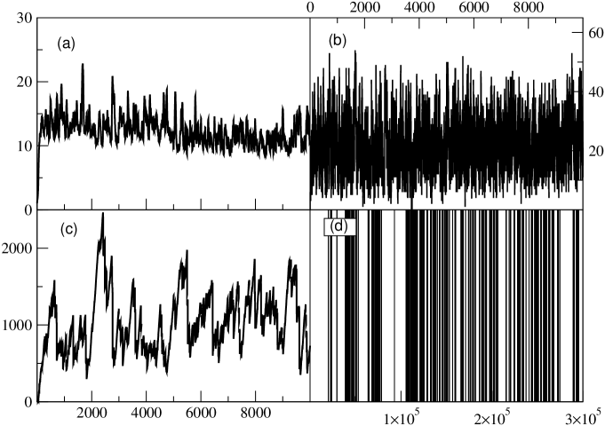
An example of time evolution of the principal characteristics of this model for the population size is shown in Fig. 1 for the following dynamical variables: (a) , (b) production of goods, (c) supply of the most wanted good, and (d) points of the ”money switching”, i.e. the points when the most wanted good is overtaken by another good. The distances between the consecutive time-points are thus to be interpreted as ”money lifetimes” within the present model. These plots are given for the threshold value which for marks a center of the region where money start emerging. From the point of view of complexity science and in relation to the financial reality, this is the most interesting region. The structure of ”money lifetimes” seen in panel (d) of Fig. 1 suggests their fractal organization and thus critical character of the transition from the phase with no money to the money phase while increasing the parameter value.
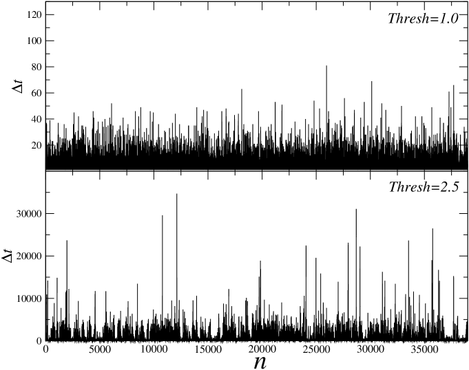
This is even more suggestive in Fig. 2 showing the consecutive ”money lifetimes” for and measured in terms of the number of trading turns. While in the former case we see a white noise-like structure with very short lifetimes, in the latter case the commodity fulfilling the criterion of money often happens to reign for up to 35000 trading turns. The overall structure in this latter case displays a characteristic ’volatility clustering’, which is a hallmark of criticality and multiscaling [17, 30]. In the following we therefore perform a more systematic quantitative study of this particular aspect of the present model using the modern formalism of multifractality [1].
3 Multifractal analysis of ”money switching” dynamics
Multiscaling [31, 32] represents a commonly accepted concept to grasp the most essential characteristics of complexity. Indeed, the related measure in terms of multifractal spectra offers an attractively compact frame to quantify the hierarchy of scales and specificity of their interwoven organization. This in particular applies to the temporal aspects of complexity and, thus, well suits the present issue of ”money switching” dynamics. Up to now there exist two main types of algorithms to determine the multifractal spectra. The one that typically delivers the most stable results [33] constitutes a natural extension of Detrended Fluctuation Analysis (DFA) [34, 35] and is known as Multifractal Detrended Fluctuation Analysis (MFDFA) [36]. The other algorithm - Wavelet Transform Modulus Maxima (WTMM) [37, 38] - is based on the wavelet decomposition of a signal. This algorithm requires more care as far as stability of the result is concerned. It at the same time offers better visualization of the relevant structures, however. For this reason, and also as a consistency test, below we use both these algorithms in parallel to analyze the same time series.
3.1 MFDFA and results
The MFDFA algorithm consists of several steps as sketched below. At first, for a time series a signal profile is calculated according to the equation:
| (2) |
where denotes averaging over a time series of length . Then the profile is divided into disjoint segments of length starting both from the beginning and from the end of the time series. For each box the assumed trend is estimated by least-squares fitting a polynomial of order . Based on our own experience (Oświȩcimka et al 2006) in the present analysis we use as optimal. Next, variance of the detrended data is calculated:
| (3) |
and finally, by averaging the function over all the segments , a th-order fluctuation function is derived according to the equation:
| (4) |
In order to determine the statistical properties of the function, the above steps are repeated for different values of . In the case of a fractal time series, fluctuation funtion reveals power law dependence: , where denotes the generalized Hurst exponent. For monofractal time series, is independent of and equals the well-known Hurst exponent . In the case of multifractal correlations, however, depends on and the Hurst exponent is obtained for . From exponents, one can calculate the multifractal spectrum according to the equations: , where denotes the Hoelder exponent and is the fractal dimension of the set of points with this particular . For multifractal time series, the singularity spectrum typically assumes shape similar to an inverted parabola whose width is considered a measure of the degree of multifractality and it thus shrinks to one point in the case of monofractal.
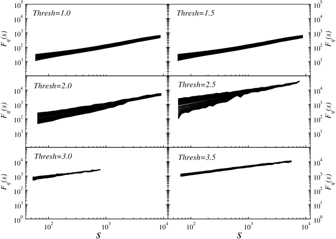
By using this method, we then address the problem of correlations in the time series of money lifetimes. For this time series (as the ones shown in Fig. 1(d) or in Fig. 2), the scale dependence for the set of the so-evaluated fluctuation functions () around the critical threshold value for the emergence of money, starting with up to with the step of 0.5, is shown in Fig. 3. As it can clearly be seen, these functions develop a power law form over the scale range of about two orders of magnitude. However, the -dependence of the corresponding power-law indices significantly varies with the threshold parameter and around this dependence (here shown for ) is the most prominent, which signals nontrivial multifractality. The degree of multifractality systematically increases while approaching this value from below, but then it sharply degrades when exceeding it.

The resulting singularity spectra are presented in Fig. 4 for the same sequence of the parameter values as in Fig. 3. Indeed, the broadest spectrum - reflecting the hightest complexity of the underlying dynamics [1] - corresponds to and departing from this value in either direction makes narrower with the maximum moving towards like for the monofractal uncorrelated signals. Comparison of these singularity spectra to the analogous quantities for the randomized (shuffled) data, shown in the inset to Fig. 4, clearly demonstrates significance of this result. After such a destruction of temporal correlations, all the spectra become narrow and located in the vicinity of . This comparison thus indicates that multifractal nature of the time series representing consecutive money lifetimes is primarily due to the long-range temporal correlations.
3.2 WTMM and results
As already mentioned above, the WTMM method is an alternative technique of detecting the fractal properties of a signal. The core of the algorithm is wavelet transform that is a convolution of a signal and a wavelet [39]:
| (5) |
where denotes a shift of the wavelet kernel and is scale. In particular, the wavelet kernel can be chosen arbitrarily. The only criterion is its good localization in space and in frequency domains. For the purpose of our analysis, we choose the third derivative of the Gaussian because it removes the trends that can be approximated by polynomials up to the second order. In the presence of singularity in the data, the scaling relation of coefficients can be observed:
| (6) |
However, this relation can be unstable in the case of densely packed singularities. Therefore, it is suggested to identify the local maxima of and then to calculate the partition function according to the equation:
| (7) |
where denotes a set of all maxima for scale and is the position of a particular maximum. In order to preserve the monotonicity of the family of the functions, the additional condition needs to be imposed:
| (8) |
In the case of fractal signals, the exponents characterize the power-law behavior of the partition function:
| (9) |
For multifractal time series is a nonlinear function of , whereas it is linear otherwise. The singularity spectrum is obtained by Legendre transforming according to the following formula:
| (10) |
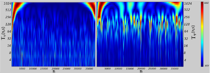
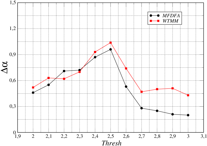
Two examples of the maps representing the wavelet transforms calculated from the same time series of money lifetimes as before for our model with and are shown in Fig. 5. The fractal character of these signals can be seen already on the visual level to manifest itself quite convincingly from the bifurcation structure of the maxima of the wavelet transform. For (right hand side of Fig. 5) the intensities of maxima vary with the scale, while for (left hand side of Fig. 5) they remain largely homogenous, which signals a more involved fractal composition in the former case. Of course, we already know from our previous MFDFA analysis that the case is strongly multifractal while the case is essentially monofractal, and here we find an alternative indication for this fact. Determining the singularity spectra according to the above-described WTMM algorithm for the same six cases of the model’s threshold parameter as in Fig. 4 gives the results shown in Fig. 6. Comparing both MFDFA and WTMM results indicates basically the same tendency even on a fully quantitative level: the broadest singularity spectrum characterizes the dynamics at around the critical threshold value for the emergence of money. These comparisons are summarized globally in Fig. 7 in terms of the threshold parameter dependence of the maximum span of the corresponding singularity spectra obtained within the MFDFA and WTMM methods. Both methods consistently point to as this value of the model’s threshold parameter (for ) where the money switching dynamics is the most complex.

4 Concluding remarks
We have performed extensive numerical simulations using the agent-based computational economic model for the creation of money, developed along the lines originally proposed by Menger [7] that money can spontaneously emerge in a commodity exchange economy. Money in this model is defined as the most wanted good. A variant of this model studied in the present paper allows emergence as well as collapse of money. This model’s ability is ruled by the only external parameter whose magnitude reflects agents tendency to act collectively and it induces memory effects. The most interesting situation takes place just at the edge between a phase with no money emergence and a phase with stable money. In this intermediate region one of the commodities spontaneously becomes universally wanted and retains such a status for sufficiently long time so that it can be considered money. Under these edge conditions the dynamics of trade is characterized by a permanent competition which leads to collapse of that particular money and another commodity overtaking. An interesting related effect that we were witnessing at the course of simulations is that such overtaking often alternates within one particular pair of commodities. In contemporary terms this can perhaps be interpreted as this model’s ability to induce effects in the spirit of competition of two currencies to become world’s leading (like USD versus Euro). From a theoretical point of view, the most interesting effect is that lifetimes of the consecutive money emerging within the model at the edge, form time series that develop remarkable multifractal characteristics as verified by the two independent algorithms: Multifractal Detrended Fluctuation Analysis (MFDFA) and Wavelet Transform Modulus Maxima (WTMM). The width of the corresponding singularity spectra (Fig. 7) considered as a function of the threshold parameter resembles the -shaped continuous phase transitions in physical systems, recently identified even in the complex networks dynamics [40]. That this transition can be paralleled to the critical phenomena is primarily indicated by an increasing span of the multifractal spectrum (and thus an increasing complexity) when approaching the transition point. The ability of the present model to generate the above effects seems very demanding since the most creative acts of Nature are commonly considered to be associated with criticality [41]. There also exists empirical evidence [42] that the consecutive intertransaction times on the stock market form time series that are multifractal. One may speculate that there is some analogy between the present ”money lifetime” issue and the stock market intertransaction times: during a given ”lifetime” money is the same; similarly, price may change only during transaction. From this perspective intertransaction time can be considered ”price lifetime”.
References
- [1] J. Kwapień, S. Drożdż, Phys. Rep. 515, 115 (2012).
- [2] Y. Aiba, N. Hatano, H. Takayasu, K. Marumo, T. Shimizu, Physica A 310, 467 (2002).
- [3] S. Drożdż, J. Kwapieṅ, P. Oświȩcimka, R. Rak, New J. Phys. 12, 105003 (2010).
- [4] S. Drożdż, A.Z. Górski, J. Kwapień, Eur. Phys. J. B 58, 499 (2007).
- [5] J. Kwapień, S. Gworek, S. Drożdż, A.Z. Górski, J. Econ. Interact. Coord. 4, 55 (2009).
- [6] V.M. Yakovenko, J.B. Jr Rosser, Rev. Mod. Phys. 81, 1703 (2009).
- [7] C. Menger. Economy J. 2 (June 1892), 239 (1892).
- [8] P. Bak, S.F. Norrelykke, M. Shubik, Quant. Finance 1, 186 (2001).
- [9] N. Kiyotaki, R. Wright, J. Political Economy 97, 924 (1985).
- [10] I. Katsuhito, Kaheiron (Theory of Money), Chikuma-Shobo, Tokyo, 1993 (in Japanese).
- [11] I. Katsuhito, Structural Change Economic Dynamics 7, 451 (1996).
- [12] A. Yasutomi, Physica D 82, 180 (1995).
- [13] A. Yasutomi, Chaos 13, 1148 (2003).
- [14] A.Z. Górski, S. Drożdż, P. Oświȩcimka, Acta Phys. Pol. A 117, 676 (2010).
- [15] E. Samanidou, E. Zschischang, D. Stauffer, T. Lux, Rep. Prog. Phys. 70, 409 (2007).
- [16] A. Chakraborti, I.M. Toke, M. Patriarca, F. Abergel, Quant. Finance 11, 1013 (2011).
- [17] T. Lux, M. Marchesi, Nature 397, 498 (1999).
- [18] G. Iori, J. Econ. Behav. Organ. 49, 269 (2002).
- [19] A. Krawiecki, J.A. Hołyst, D. Helbing, Phys. Rev. Lett. 89, 158701 (2002).
- [20] J.-S. Yang, O. Kwon, W.-S. Jung, I. Kim, Physica A 387, 5498 (2008).
- [21] M. Denys, T. Gubiec, R. Kutner, Acta Phys. Pol. A 123, 513 (2013).
- [22] K. Kacperski, J.A. Hołyst, J. Stat. Phys. 84, 169 (1996).
- [23] D. Helbing, I. Farkas, T. Vicsek T, Nature 407, 487 (2000).
- [24] K. Sznajd-Weron, J. Sznajd, Int. J. Mod. Phys. C 11, 1157 (2000).
- [25] A. Grabowski, R.A. Kosiński, Physica A 361, 651 (2006).
- [26] P. Gawroński, K. Kułakowski, Comp. Phys. Comm. 182, 1924 (2011).
- [27] J.-P. Bouchaud, Nature 455, 1181 (2008).
- [28] J.D. Farmer, D. Foley, Nature 460, 685 (2009).
- [29] T. Lux, F. Westerhoff, Nature Phys. 5, 2 (2009).
- [30] S. Drożdż, J. Kwapień, P. Oświȩcimka, R. Rak, Europhys Lett (EPL) 88, 60003 (2009).
- [31] T.C. Halsey, M.H. Jensen, L.P. Kadanoff, I. Procaccia, B.I. Shraiman, Phys. Rev. A 33, 1141 (1986).
- [32] H.G.E. Hentschel, I. Procaccia, Physica D 8, 435 (1983).
- [33] P. Oświȩcimka, J. Kwapień, S. Drożdż, Phys. Rev. E 74, 016103 (2006).
- [34] C.K. Peng, S.V. Buldyrev, S. Havlin, M. Simons, H.E. Stanley, A.L. Goldberger, Phys. Rev. E 49, 1685 (1994).
- [35] J.W. Kantelhardt, E. Koscielny-Bunde, H.H.A. Rego, S. Havlin, A. Bunde, Physica A 295, 441 (2001).
- [36] J.W. Kantelhardt, S.A. Zschiegner, A. Bunde, S. Havlin, E. Koscielny-Bunde, H.E. Stanley, Physica A 316, 87 (2002).
- [37] J.F. Muzy, E. Bacry, A. Arneodo, Int. J. Bifurcation Chaos 04, 245 (1994).
- [38] A. Arneodo, E. Bacry, J.F. Muzy, Physica A 213, 232 (1995).
- [39] A. Grossmann, J. Morlet, S.I.A.M. J. Math. Anal. 15, 723 (1984).
- [40] M. Wiliński, B. Szewczak, T. Gubiec, R. Kutner, Z.R. Struzik, Eur. Phys. J. B 88, 34 (2015).
- [41] P. Bak, How Nature works: the science of self-organized criticality, Springer-Verlag, New York, 1996.
- [42] P. Oświȩcimka, J. Kwapień, S. Drożdż, Physica A 347, 626 (2005).