A biaxial apparatus for the study of heterogeneous and intermittent strains in granular materials

Abstract

We present an experimental apparatus specifically designed to investigate the precursors of failure in granular materials. A sample of granular material is placed between a latex membrane and a glass plate. A confining effective pressure is applied by applying vacuum to the sample. Displacement-controlled compression is applied in the vertical direction, while the specimen deforms in plane strain. A Diffusing Wave Spectroscopy visualization setup gives access to the measurement of deformations near the glass plate. After describing the different parts of this experimental setup, we present a demonstration experiment where extremely small (of order $10^{-5}$) heterogeneous strains are measured during the loading process.

1 Introduction

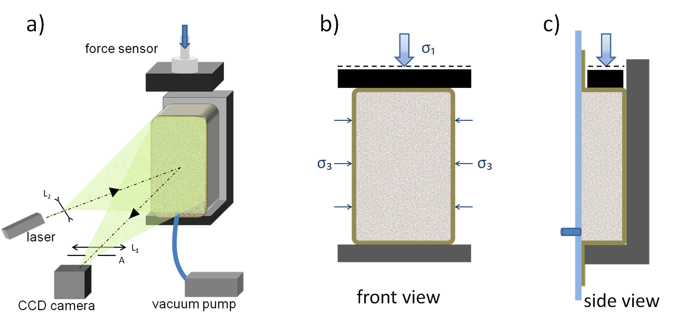
Figure 1: Sketch of the experimental setup. The material is placed between a glass plate and a latex membrane. (a) The front is illuminated by a laser beam which is expended by the lens $L_{2}$ in order to light the whole sample. Multiple light scattering occurs in the grains assembly and part of the light is backscattered. The front side of the sample is imaged by the lens $L_{1}$ on the CCD camera. The size of the speckle spots is controlled by the diaphragm aperture A. The vacuum pump maintains a depressurization inside the sample at the origin of the stress $\sigma_{3}$ on the lateral walls. A force sensor on the top of the loading plate measures the stress $\sigma_{1}$ corresponding to the imposed displacement. (b) Front view with the applied stresses. (c) Side view showing the plane strain configuration: the displacements are blocked by the front (glass plate) and back walls.

Describing the mechanical behavior of granular materials is a very challenging task, especially when dealing with strain localization phenomena that eventually leads to macroscopic failure. Strain localization (often referred to as shear banding) has quite a practical relevance, as stability and deformation characteristics of earth structures are often controlled by the soil behavior within the zones of localized strain schofield ; davis ; nedderman . Yet, the mechanisms responsible for the formation of these zones in granular materials are still subject to debate. While the formation of a shear band is now generally interpreted as a bifurcation problem in continuum mechanics (e.g. rice1976 ; rudnicki1975 ), its theoretical and numerical treatment still presents special problems for granular materials ( see for example the monograph by Vardoulakis and Sulem  vardoulakis and the review paper by Bésuelle and Rudnicki besuelle2004 ). While the issues of orientation and thickness of shear bands have been debated for decades, other, more intricate issues have more recently attracted the interest of experimental research in this field: among the others, the occurrence of temporary or non-persistent modes of localization, that is, localized regions which form during the test and eventually disappear (see for example hall2010 ). From an experimental standpoint, temporary modes of strain localization are inherently more difficult to observe and characterize than final, persistent shear bands. Not only they transient, but they are also characterized by less intense shear strain. Many optical methods are available for measuring strain fields in a deforming granular assembly (see viggiani2012 ). However, many of them fail to detect these temporary patterns of strain localization, because their spatial and temporal resolution is not fine enough (it should be mentioned, though, that recently the performance of (Digital Image Correlation) DIC based methods has been significantly improving thanks to the increasingly higher resolution of existing cameras). In this paper, we present a full-field method that has the capability to detect fine non persistent regions of localized strain. First we present the experimental setup, specifically designed to resolve strains as small as $10^{-5}$, as well as the interferometric method for measuring strain (Section 2). In section 3 we discuss the experimental protocols, and in Section 4 we discuss the results of a typical experiment, showing the potential of the experimental setup.

2 Experimental setup

2.1 Overview of the setup

The experimental setup consists of a plane strain apparatus coupled with a dynamic light scattering setup. The schematic drawing of the setup is shown in fig. 1. The granular material is placed between a latex membrane and a glass plate, and a vacuum is applied in the granular material. A confining effective pressure $\sigma_{3}$ results from the applied vacuum. The granular material is compressed on the top through the displacement of a plate. The displacement of the top plate and the force exerted on it are measured during the compression. In front of the apparatus, on the side of the glass window, a light scattering setup is placed. The front of the granular material is illuminated with an extended laser beam. The light which is scattered by the granular material is recorded by a camera imaging the front of the sample. We analyze the scattered light in order to access to information about the deformation of the granular material.

2.2 Mechanical part

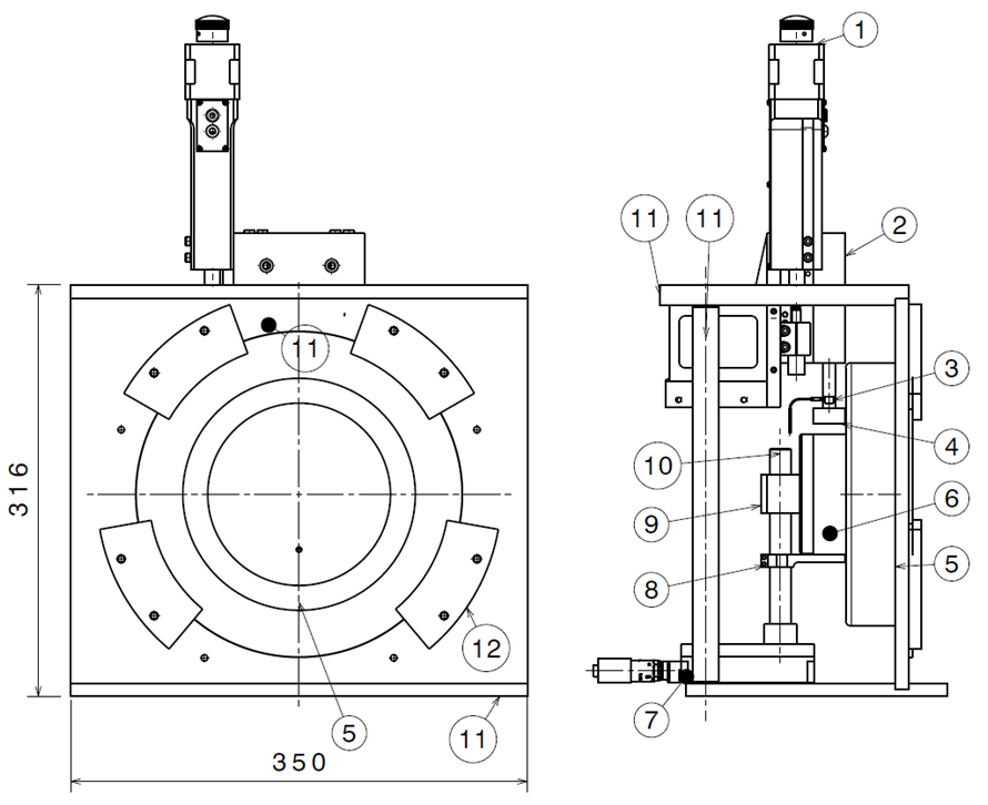
Figure 2: Front (left) and side (right) views of the biaxial apparatus. {\tiny1}⃝ motor, \tiny2⃝ motorized translation stage, \tiny3⃝ force sensor, \tiny4⃝ loading plate, \tiny5⃝ glass window, \tiny6⃝ sample of granular material, \tiny7⃝ translation stage, \tiny8⃝ bottom plate, \tiny9⃝ back plate, \tiny10⃝ positioning axis, \tiny11⃝ structure, \tiny12⃝ wedges holding the glass window.

The drawing of the mechanical part of the setup is shown on fig. 2. The granular sample (fig. 2 \tiny6⃝) of size $(85\times 55\times 25)$mm³ is submitted to a biaxial test in plane strain conditions. To limit the gravity effects and homogenize the force along out-of-the-plane direction, the granular matter is maintained by depressurization between a glass plate and a latex membrane. A motorized translation stage (fig. 2 \tiny1⃝-\tiny2⃝, Thorlabs) is used for the compression. The loading plate (fig. 2 \tiny4⃝) is fixed on the linear long-travel translation stage (fig. 2 \tiny2⃝, Thorlabs LNR50 Series) which is driven by a stepper motor (DC Servo Motor Actuator, Thorlabs DRV414). The DC Motor Controller (Thorlabs BDC101) allows to pilot the translation stage. The two main controls are the speed of the stage (length of the step per second) and the stop position. Between the loading plate and the translation stage a $500$ N force sensor (fig. 2 \tiny3⃝, Measurements Specialities) gives the force applied on the sample.

2.3 Spatially resolved Diffusing Wave Spectroscopy

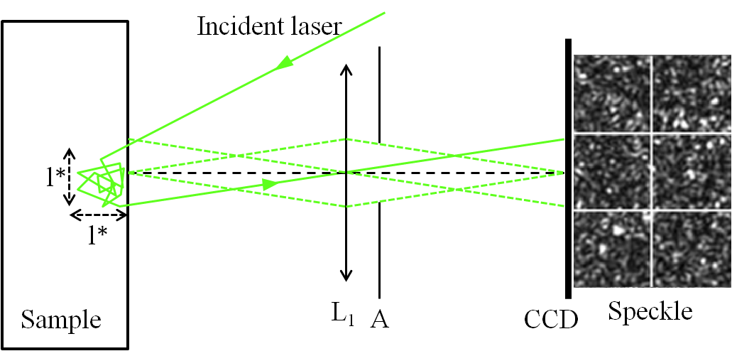
Figure 3: Example of an incident ray path undergoing multiple scattering inside the granular media and backscattered through the lens and the diaphragm aperture on the camera. Right: example of 6 meta-pixels of the speckle pattern recorded with the camera.

The measurement of the deformation of the granular material is obtained with a spatially resolved home-made Diffusing Wave Spectroscopy (DWS) setup described in detail elsewhere erpelding2008 . DWS is an interference technique using scattering of coherent light by strongly diffusive materials. A light beam emerging from a laser source enters the sample (fig. 3), and is scattered many times. The different exiting rays interfere on the camera sensor and produce a speckle pattern consisting of dark and bright spots (see right part of fig. 3). A displacement of the scatterers modifies the path length of the rays. This produces changes in the phases of the scattered waves. Those phase variations induce modifications of the speckle pattern. The variation of the speckle pattern is then characterized by the computing of the correlation function of the scattered light.

As shown in fig. 1.a, we are in a backscattering geometry for DWS, meaning that the backscattered light is collected. In practice, the glass window side of the sample is illuminated by a laser source of wavelength $\lambda=532$ nm and maximum output power 75 mW (Compass 215M from Coherent). The beam is expanded with the lens $L_{2}$ (see fig. 1.a) in order to illuminate the whole front face of the sample. The image of the front is done using a lens $L_{1}$ of focal length 100 mm, allowing a magnification in agreement with the whole optical system (sample-camera). The speckle pattern is recorded with a camera (PT-41-04M60 from DALSA) with $2352\times 1728$ resolution and pixel size $7.4\mu m$.

Speckle analysis.

The speckle pattern is recorded by the camera. Correlations of the scattered intensities are calculated between two images $1$ and $2$ in the following way. First the speckle images are divided into square regions that we called meta-pixels (see image on right of fig. 3). For each meta-pixel, the correlation function $g^{(12)}_{I}$ between the two intensities $I_{1}$ and $I_{2}$ is computed as,

$$g^{(12)}_{I}=\frac{\left\langle I_{1}I_{2}\right\rangle-\left\langle I_{1}\right\rangle\left\langle I_{2}\right\rangle}{\sqrt{\left\langle I^{2}_{1}\right\rangle-\left\langle I_{1}\right\rangle^{2}}\sqrt{\left\langle I^{2}_{2}\right\rangle-\left\langle I_{2}\right\rangle^{2}}},$$ (1)

where $I_{1}$ and $I_{2}$ are the matrices of intensities of the meta-pixel considered, and averages are performed over all the pixels of the meta-pixel. The correlation function (eq. (1)) is normalized so that $g^{(12)}_{I}=1$ if $I_{1}=I_{2}$, and $g^{(12)}_{I}=0$ if the intensities are uncorrelated. The link between the displacements of the beads and the value of the correlation function may be estimated from a model of light propagation into the granular material. As the bead assembly strongly scatters light, rays follow random walks inside the material. The transport mean free path, i.e. the persistent length of the random walk of light in the material is denoted by $l^{*}$. Typically, for a granular material, this optical constant is few diameters of grains. We will discuss the value of $l^{*}$ and its implication on the spatial resolution of the deformation maps that we obtain in sec. 3.3. If the deformation of the material between the two images 1 and 2 can be considered as affine and homogeneous on the scale of a metapixel, the correlation function can be expressed in backscattering geometry as djaoui2005 ; crassous2007 ; erpelding2008 :

$$\left|g^{(12)}_{I}\right|\approx exp\Bigl{(}-\eta kl^{*}\sqrt{f({\bf U})}\Bigr{)},$$ (2)

where $\eta$ is an optical factor of order 1, and $f({\bf U})={1\over 5}Tr^{2}({\bf U})+{2\over 5}Tr({\bf U}^{2})$ is a function of the invariant of the strain tensor ${\bf U}=\frac{1}{2}\left(\frac{\partial u_{i}}{\partial x_{j}}+\frac{\partial u_{j}}{\partial x_{i}}\right)$. If the bead displacements is the sum of an affine motion with a strain tensor $\bf U$ and an uncorrelated motion of the beads, we then expect bicout1994 :

$$\left|g^{(12)}_{I}\right|\approx exp\Bigl{(}-\eta k\sqrt{(l^{*})^{2}f({\bf U})+\langle\Delta r^{2}\rangle}\Bigr{)},$$ (3)

with $\langle\Delta r^{2}\rangle$ the average of the quadratic displacement of the uncorrelated motion of the beads.

3 Experimental Protocol

Here we summarize the different steps of the protocol of fabrication of the latex membrane and of preparation of the granular material. The limitations and the sensitivity of both the mechanical device and the optical setups are detailed. The control of the camera and the acquisition of images, the force sensor monitoring and the displacement control are all ensured by a Labview interface on a computer.

3.1 Preparation of the membrane and granular sample

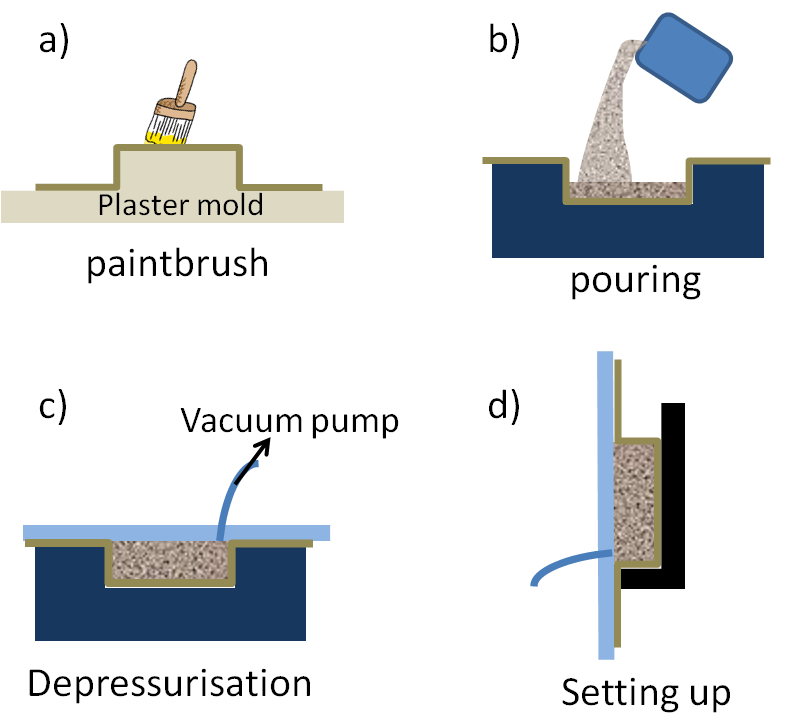
Figure 4: Steps for preparing a sample. (a) Confection of the latex membrane on a plaster mold. (b) The latex membrane is fitted into a counter mold and the granular material is poured and possibly compacted. (c) The glass plate is laid overall, and partial vacuum is created in the sample. (d) The sample is placed on the biaxial apparatus.

As shown in fig. 4.a, the latex membrane is made by spreading successive layers of liquid latex with a paintbrush on a plaster mold of the required dimensions. After drying it generates a planar membrane with a hollow of the size of the sample. The same membrane can be used for several tests. To prepare the sample, the membrane is laid in a counter-mold horizontally and the granular material is poured in the hollow (fig. 4.b). A compaction protocol is applied to the pile according to the desired volume fraction. The glass plate is then placed over the membrane (fig. 4.c). A flexible pipe connects the vacuum pump to the glass plate and the sample is pressed on the glass instantly by depressurization. We use vacuum grease between the annular part of the latex membrane and the glass plate for better sealing and adherence. The grease is viscous and does not creep into the bulk solid during the whole time of the experiment. A pressure sensor and an air valve allow the measurement and control of the depressurization using a feedback loop. Then the window (fig. 2 \tiny5⃝), bearing the sample, is fixed on the structure of the biaxial apparatus using wedges (fig. 2 \tiny12⃝). Because of residual air leakages and long duration experiments, the pump and the pressure control system are active during the whole loading experiment. To achieve plane strain conditions, the back plate and the bottom plate are brought in contact with the sample using a translation stage (fig. 2 \tiny7⃝). The loading is applied using a plate larger than the sample in the $\sigma_{3}$ direction (more than 55 mm, see fig. 1.b), and slightly smaller than the sample thickness in the other direction (less than 25 mm, see fig. 1.c). The distances between the glass plate and the loading plate on one hand and between the back plate and the loading plate on the other hand are approximately of 1 mm. Our apparatus does not give the position of the granular material with respect to the motorized translation stage \tiny2⃝.

3.2 Mechanical stiffness of the system

Several tests have been conducted to characterize the apparatus. The range of the force sensor is limited to 500 N and its calibration has been made using known loads. Its stiffness has been investigated and the spring constant of the sensor has been measured in two different ways. First, using a stiff micrometer stage we have imposed a known deformation to the sensor, and have measured the force on the sensor. We obtained a stiffness for the sensor of $k_{sens}=(4.3\pm 0.2)\times 10^{6}$ N.m^-1. We have also tracked the deformation of the sensor by following the displacement of markers above and below the sensor using a method described in chean2011 , and have measured $k_{sens}=(5\pm 1)\times 10^{6}$ N.m^-1. Other tests were conducted to measure the stiffness of the bottom plate and the stiffness of the whole loading device. The stiffness of the whole system has been tested in a Hertz contact configuration and is found to be $k_{sys}=7.3\times 10^{5}$ N.m^-1. The stiffness of a block of material of section $S$, length $L$ and of Young modulus $E$ is $k_{mat}=SE/L$. For $S\approx 1.4\times 10^{-3}$ m² and $L\approx 85$ mm, $k_{sys}=k_{mat}$ for $E=44$ MPa. This gives an estimation of the limit value of the Young modulus above which the correction due to the apparatus stiffness must be taken into account. The motorized linearized stage is limited to one step of 1 $\mu$m per second and to a maximal loading of $250~{}N$. Tests confirm this value, with an activation of security around $240~{}N$. Estimation of the membrane rigidity from the values of latex elastic modulus show that the elasticity of the membrane is negligible.

3.3 Optical protocol and sensitivity

The first optical issue is to acquire a suitable speckle pattern. The focal length of the lens and the distances between the sample, the lens and the camera have to be in agreement with the magnification allowing to image the whole surface of the sample on the camera. Then the diaphragm aperture (see fig. 3) allows adjustment of the size of the speckle spots. This size is determined from the Fourier transform of the image of intensity. The size of the speckle spot is fixed to $\approx 2.3$ pixels which is a good compromise between the necessity to have the maximum number of speckle spots, and the need for the speckle spots to be at least few pixels.

Concerning the time resolution, the stepper motor frequency is limited to one step per second, the acquisition rate of the images to $4$ frames per second, and we acquire $1$ image per motor step. The correlation maps are calculated between 2 images using eq. (1). These two images can be spaced out by a specific time interval.

The spatial resolution of the deformation map that we obtain is dependent on both the camera used and of the granular material. As for the camera, the correlation functions must be calculated on large enough areas in order to minimize the statistical error when evaluating eq. (1). In practice, the noise on the correlation function is kept to an acceptable level if the size of a meta-pixel is at least $16\times 16$ pixels. With a speckle size of $2.3$ pixels, this corresponds to $\sim 50$ speckle spots per metapixel. Concerning the material, the resolution is limited by the light scattering process inside the granular media. Photons that enter the granular material at a given point typically exit the media at a distance smaller or of order $l^{*}$ and have mainly probed zones inside the material of size $l^{*}$. So, as shown on fig. 3, a photon that emerges from a given point of the material have explored a volume of order $(l^{*})^{3}$. The information about the deformation of the material is thus naturally averaged over this volume as shown in fig. 3. The spatial resolution is thus limited to $l^{*}$ by the scattering process. The optimal choice of the optical setup is when a meta-pixel on the camera is the image of an area of order $l^{*}\times l^{*}$ on the object. If we call $L$ the largest dimension of the material sample, the optimum of resolution is attained with our $2352$ pixel width camera when $L/l^{*}=2352/16\simeq 150$. For a sample size of $L=85$ mm, this corresponds to an optimal value of $l^{*}\simeq 0.6$ mm. For spherical glass beads, model of light propagation into granular material crassous2007 and experiments crassous2007 ; djaoui2005 ; amon2013 show that $l^{*}\simeq 3.3$ $d$, with $d$ the mean bead diameter. For Fontainebleau sand, we measured $l^{*}\simeq 2.0~{}d$ amon2013 . So optimal value for grains diameter is typically $d=200-300\mu m$ depending on the material.

It should be stressed that those resolution considerations hold for the best spatial resolution. With this resolution, one meta-pixel corresponds to deformation that are averaged on typical sizes of $l^{*}$ i.e. of few $d$. Larger beads may be also used: we made DWS studies with glass beads of diameter $d=500~{}\mu$m in a different experimental geometry crassous2008 ; richard2008 . Smaller beads may also be used but with a spatial resolution larger than $l^{*}$. Keeping the same spatial resolution may however be achieved by zooming on a smaller part of the sample, or with an image acquisition device with better spatial resolution such as high resolution camera.

4 A demonstration experiment

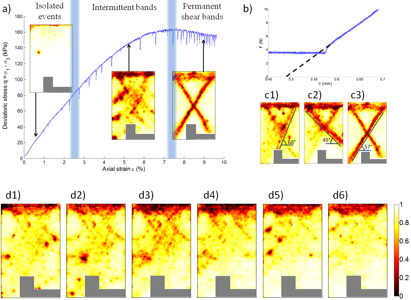
Figure 5: (a) Loading curve: Difference of stresses $q=\sigma_{1}-\sigma_{3}$ versus vertical strain $\epsilon$ for a confining stress $\sigma_{3}=30$ kPa and associated correlation maps computed for an incremental vertical strain of $\Delta\epsilon\simeq 1.2\cdot 10^{-5}$. (b) Zoom of the beginning of the loading process. The offset position for the displacement is defined from the extrapolation at zero applied force. (c) Different maps of correlation showing deformation bands with different angles of inclination (see text). (d) Successive snapshots of deformation showing the intermittency of the deformation map (see text) and the correlation function $g_{I}$ colorscale.

In order to show the potential of the apparatus that we built, we propose here a demonstration experiment where we compress a model granular system made of cohesionless nearly spherical glass beads.

4.1 Settings

We used for this experiment glass beads of $200-300\mu m$ diameter in a membrane of dimension $85$ mm height, $55$ mm width and $25$ mm depth. Concerning the preparation of the sample, the grains are poured inside the membrane and then softly shaken by hand for a regular compaction before the depressurization. The confining pressure is fixed to a value $\sigma_{3}=30$ kPa. Using the mean value of the grains diameter, the transport mean free path can be estimated to $l^{*}\approx 0.66~{}mm$. The obtained image is divided in squares of $16\times 16$ pixels which correspond to squares of $(0.64\times 0.64)mm^{2}$ on the sample. The typical noise of the correlation function $g_{I}$ is $0.03$. For a quasi-static loading we chose for the velocity of the top plate $1\mu m/s$ which is approximately an vertical strain of $1.2\cdot 10^{-5}$ between $2$ motors steps. We acquire one frame per second.

4.2 Stress strain curve

The loading curve showing the difference of stresses versus the vertical strain is presented on fig. 5.a. The vertical strain is obtained as $\epsilon=(\delta-\delta_{0})/L$, with $L=85$ mm and $\delta$ the loading plate displacement. The value of the offset of displacement $\delta_{0}$ for which the vertical deformation $\epsilon$ is null is determined by the linear extrapolation of the force-displacement curve at zero force (see fig.5.b). The difference of stresses $q=\sigma_{1}-\sigma_{3}$ is obtained using $q=F/S$, with $F$ the measured force, and $S=1.37\times 10^{-3}~{}m^{2}$ the section of the material. The stress versus strain curve of the material is typical of soil mechanics experiments, with first a quasi-linear part. Then the slope decreases until a maximum of the curve is reached, followed by a slow stress relaxation. We also observe small stress drops during the loading process. Such stress drops are not systematically observed. In some similar experiments not shown here, we do not observe them during the loading. Such drops are reported in the literature amon2012 , they correlate typically with an instability in part of the force network. This is in agreement with the fact that we do not observe them during the compression of a bulk elastic material of same Young modulus value.

4.3 Strain maps

Some typical maps of correlations between two successive images (corresponding to an vertical strain increment of $\Delta\epsilon\simeq 1.2\cdot 10^{-5}$) are shown on fig. 5.d.

These are roughly representative of the three distinct ways to deform. At the beginning of the loading, we first observe a background of deformation with some isolated reorganizations already observed and described in another experiment amon2012 . At a vertical deformation of order $\epsilon\simeq 0.02$, we begin to see some decorrelated areas that occur in the form of small bands. Such bands are intermittent: they appear and disappear as the loading proceeds. The positions of such bands seem to be arbitrary: the ending points may be on the boundaries of the sample or not. Those bands may cross each other, or a band may start from another one. We observe several orientations (see fig. 5.c1 and c2) from $\simeq 45^{\circ}$ to $\simeq 68^{\circ}$. A $45^{\circ}$ angle corresponds to the Roscoe angle $\theta_{R}$ for non dilating material. Those bands share some analogies with the micro-bands described by Kuhn kuhn1999 or Tordesillas tordesillas2008 in numerical Discrete Element Method (DEM) simulations. More inclined bands with a angle $\simeq 68^{\circ}$ are also observed. This angle is in agreement with the angle of shear bands predicted by the Mohr-Coulomb criterium $\theta_{C}=45^{\circ}+\phi/2\simeq 68^{\circ}$, with $\sin\phi=(\sigma_{1}-\sigma_{3})/(\sigma_{1}+\sigma_{3})\simeq 0.733$ at the maximum load. At the end of the loading, we observe two permanent symmetric bands which start from the corners of the sample, and form the shape of the letter X. Their inclination is $\simeq 57^{\circ}$ (see fig.5.c3). We note $\theta_{G}$ this geometric angle. Such symmetric bands are widely reported in the literature. Near the loading peak the situation is confused, displaying intermittent bands at $\theta_{R}$ and $\theta_{C}$ but also some parts of the future permanent bands at $\theta_{G}$.

4.4 Intermittency

In conventional biaxial test experiments, the map of strain is measured during axial (vertical) strain increments of typically $\Delta\epsilon\sim 10^{-3}$. The great sensitivity of our optical method for strains measurement allows the determination of strain for vertical deformation increments as small as typically $\Delta\epsilon\sim 10^{-5}$. As a consequence we are able to investigate the instantaneous micro-deformations of the sample. This is an important difference with more conventional setup. The instantaneous deformation seems to show important temporal fluctuations during the loading. Figure 5.d shows six consecutive instantaneous maps of deformation around the mean vertical strain $\epsilon_{0}=3.74\cdot 10^{-2}$. The deformation maps correspond to successive vertical strain increment, i.e. the image $d_{i}$, for $i=1$ to $6$ corresponds to map of deformation between vertical strain $\epsilon_{0}+(i-1)\Delta\epsilon$ and $\epsilon_{0}+i\Delta\epsilon$ with $\Delta\epsilon\simeq 1.2\cdot 10^{-5}$. As it can be seen in fig. 5.d the areas of instantaneous deformation fluctuate strongly. The typical size of the heterogeneities and the inclination of the bands of localized strain are roughly the same during the snapshot sequence. However the positions of these zones fluctuate strongly from one image to the other. This seems to indicate that this part of the loading is associated to some kind of intermittent deformation of the granular material. In contrast, the shear bands observed after the load peak are rather permanent, and do not show very important fluctuations.

5 Conclusions and future work

We presented in this paper a biaxial apparatus that designed to measure tiny deformations in granular samples. By analysing the evolution of the scattered light, we are able to obtain a map of the deformation of the granular material. The level of correlation is related to the local affine deformation of the material and to the fluctuations of positions around this affine deformation. Finally a test experiment on a granular material composed of glass spheres shows that deformation modes during an increment of vertical deformation are very various.

The obtained information about the deformations of the material is different from similar experiments using more conventional DIC methods see e.g. desrues2004 ; rechenmacher2006 ). We do not track individually the positions of the particles. Moreover, information on the separate component of the strain tensor are not obtained: we are not, for example, able to distinguish between small dilatation or shear of the material. However, the ability to measure small incremental deformations allows to obtain a very different information on the material deformation. The emergence of localization may be tracked at the early stages of the deformation where conventional DIC is limited to deformation during large strain increment near the load peak, though evolutions are in progress with very high resolution cameras. If necessary, the tracking of individual particles on a part of the front face may be obtained to complement the DWS interferometric imaging. For this, images in white light have to be recorded by the same or by another camera.

We focused in this paper on the description of the apparatus and on the experimental methods. Our demonstration experiment shows a very complex road leading to the failure, with numerous regimes of shear bands inclinations. In future work, we will investigate experimentally the evolution of those intermittent micro-failures toward the final rupture in a simple nearly mono-disperse and non cohesive granular material made of glass beads. Studies on cohesive material or on the nucleation of failure from a defect inside the material may also be considered with our apparatus.

- (1) A.N.Schofield and C.P.Wroth. Critical State Soil Mechanics. McGraw-Hill, 1968.
- (2) R.O.Davis and A.P.S.Selvadurai. Plasticity and geomechanics. Cambridge University Press, 2002.
- (3) R.M.Nedderman. Statics and Kinematics of Granular Materials. Cambridge University Press, 1992.
- (4) J.R.Rice. The localization of plastic deformation. In Koiter, editor, Theoretical and Applied Mechanics, pages 207–220. North-Holland Publishing: Amsterdam, 1976.
- (5) J.W.Rudnicki and J.R.Rice. Conditions for the localization of deformation in pressure-sensitive dilatant materials. Journal of the Mechanics and Physics of Solids, 23:371 394, 1975.
- (6) I.Vardoulakis and J.Sulem. Bifurcation analysis in geomechanics. Blackie Academic and Professional, Glasgow, England, 1995.
- (7) P.Bésuelle and J.W.Rudnicki. Localization: Shear bands and compaction bands. In Y.Guéguen and M.Boutéca, editors, Mechanics of Fluid-Saturated Rocks, pages 219–321. International Geophysics Series vol.89, Academic Press., 2004.
- (8) S.A.Hall, D.W.Muir, E.Ibraim, and G.Viggiani. Localised deformation patterning in 2d granular materials revealed by digital image correlation. Granular Matter, 12:1–14, 2010.
- (9) G.Viggiani and S.A.Hall. Full-field measurements in experimental geomechanics: historical perspective, current trends and recent results. In E.Romero, editor, Advanced experimental techniques in geomechanics, pages 3–67. 2004.
- (10) M.Erpelding, A.Amon, and J.Crassous. Diffusive wave spectroscopy applied to the spatially resolved deformation of a solid. Phys. Rev. E, 78:046104, Oct 2008.
- (11) L.Djaoui and J.Crassous. Probing creep motion in granular materials with light scattering. Granular Matter, 7:185–190, 2005. 10.1007/s10035-005-0210-5.
- (12) J.Crassous. Diffusive wave spectroscopy of a random close packing of spheres. Eur. Phys. J. E, 23:145–152, 2007.
- (13) D.Bicout and G.Maret. Multiple light scattering in taylor-couette flow. Physica A, 210:87–112, 1994.
- (14) V.Chean, E.Robin, R.El Abdi, J.-C.Sangleboeuf, and P.Houizot. Use of the mark-tracking method for optical fiber characterization. Optics and Laser Technology, 43:1172–1178, 2011.
- (15) A.Amon, R.Bertoni, and J.Crassous. Experimental investigation of plastic deformations before a granular avalanche. Phys. Rev. E, 87:012204, Jan 2013.
- (16) J.Crassous, J.-F.Metayer, P.Richard, and C.Laroche. Experimental study of a creeping granular flow at very low velocity. Journal of Statistical Mechanics: Theory and Experiment, 2008(03):P03009, 2008.
- (17) P.Richard, A.Valance, J.-F.Métayer, P.Sanchez, J.Crassous, M.Louge, and R.Delannay. Rheology of confined granular flows: Scale invariance, glass transition, and friction weakening. Phys. Rev. Lett., 101:248002, Dec 2008.
- (18) A.Amon, V.B.Nguyen, A.Bruand, J.Crassous, and E.Clément. Hot spots in an athermal system. Phys. Rev. Lett., 108:135502, Mar 2012.
- (19) M.R.Kuhn. Structured deformation in granular materials. Mechanics of Materials, 31(6):407 – 429, 1999.
- (20) A.Tordesillas, M.Muthuswamy, and S.Walsh. Mesoscale measures of nonaffine deformation in dense granular assemblies. Journal of Engineering Mechanics, 134(12):1095–1113, 2008.
- (21) J.Desrues and G.Viggiani. Strain localization in sand: an overview of the experimental results obtained in grenoble using stereophotogrammetry. International Journal for Numerical and Analytical Methods in Geomechanics, 28(4):279–321, 2004.
- (22) A.L.Rechenmacher. Grain-scale processes governing shear band initiation and evolution in sands. Journal of the Mechanics and Physics of Solids, 54(1):22 – 45, 2006.