Abstract

Voigt wave propagation (VWP) was considered in a porous biaxial dielectric material which was infiltrated with a material of refractive index $n_{a}$. The infiltrated material was regarded as a homogenized composite material in the long-wavelength regime and its constitutive parameters were estimated using the extended Bruggeman homogenization formalism. In our numerical studies, the directions which support VWP were found to vary by as much as $300^{\circ}$ per RIU as the refractive index $n_{a}$ was varied. The sensitivities achieved were acutely dependent upon the refractive index $n_{a}$ and the degrees of anisotropy and dissipation of the porous biaxial material. The orientations, shapes and sizes of the particles which constitute the infiltrating material and the porous biaxial material exerted only a secondary influence on the maximum sensitivities achieved. Also, for the parameter ranges considered, the degree of porosity of the biaxial material had little effect on the maximum sensitivities achieved. These numerical findings bode well for the possible harnessing of VWP for optical sensing applications.

Keywords: Voigt waves, extended Bruggeman homogenization formalism, optical sensing

1 Introduction

Voigt wave propagation (VWP) is an example of a singular form of optical propagation. In the nonsingular case of optical propagation in a linear, homogeneous, anisotropic, dielectric material, two independent plane waves, with orthogonal polarizations and different phase speeds, generally propagate in a given direction [1]. However, in certain dissipative biaxial dielectric materials, for example, there exist particular directions along which these two waves coalesce to form a single plane wave, namely a Voigt wave [2, 3, 4, 5, 6, 7]. Most conspicuously, the amplitude of this Voigt wave varies linearly with propagation direction. More complex materials, such as bianisotropic materials, offer greater scope for VWP [8, 9], but we restrict our attention here to the relatively simple case involving biaxial dielectric materials.

While VWP constitutes a fundamental phenomenon in the optics of anisotropic (and bianisotropic) materials, these waves have yet to be exploited in technological applications. However, recent advances relating to engineered composite materials may lead to VWP being more readily harnessed for technological applications. For example, homogenized composite materials (HCMs) may be conceptualized which support VWP, with these HCMs being derived from relatively commonplace component materials which do not themselves support VWP [10, 11]. Furthermore, by judicious design of the homogenization process, the directions in the HCM which support VWP may be controlled [12].

The present study is motivated by the prospect harnessing VWP for optical sensing applications. Specifically, a porous biaxial dielectric material is considered; and we investigate how the directions which support VWP vary as the porous material is infiltrated by a material of refractive index $n_{a}$. The infiltrated porous material is regarded as an HCM. An extended version of the Bruggeman homogenization formalism is used to estimate the HCM’s constitutive parameters [13]. This formalism accommodates particulate component materials where the component particles may have different shapes, orientations and sizes, and it is not restricted to small volume fractions of the infiltrating material.

In our notation, bold typeface denotes a vector, with the $\hat{}$ symbol signifying a unit vector. Thus, $\hat{{\bf x}}$, $\hat{{\bf y}}$ and $\hat{{\bf z}}$ represent the unit Cartesian vectors. Double underlining with normal typeface denotes a 3$\times$3 dyadic; and $\underline{\underline{I}}=\hat{{\bf x}}\,\hat{{\bf x}}+\hat{{\bf y}}\,\hat{{\bf y}}+\hat{{\bf z}}\,\hat{{\bf z}}$ is the identity 3$\times$3 dyadic. The superscript $T$ denotes the dyadic transpose; and the dyadic operator ‘det’ yields the determinant. Double underlining with blackboard bold typeface denotes a 6$\times$6 dyadic. The symbols $\epsilon_{\scriptscriptstyle 0}$ and $\mu_{\scriptscriptstyle 0}$ represent the permittivity and permeability of free space, respectively, while the free-space wavenumber is given as $k_{\scriptscriptstyle 0}=\omega\sqrt{\epsilon_{\scriptscriptstyle 0}\mu_{\scriptscriptstyle 0}}$, with $\omega$ being the angular frequency.

2 Homogenization formalism

2.1 Component materials

Let us consider an HCM arising from two component materials, labelled $a$ and $b$. Suppose that component material $a$ is an isotropic dielectric material with permittivity dyadic $\underline{\underline{\epsilon}}_{\,a}=\epsilon_{\scriptscriptstyle 0}\epsilon_{a}\underline{\underline{I}}$, where the relative permittivity $\epsilon_{a}=n^{2}_{a}$. Component material $b$ is taken to be an orthorhombic dielectric material characterized by the diagonal permittivity dyadic [14]

$$\underline{\underline{\epsilon}}_{\,b}=\epsilon_{\scriptscriptstyle 0}\left[\,\epsilon^{x}_{b}\,\hat{{\bf x}}\,\hat{{\bf x}}+\epsilon^{y}_{b}\hat{{\bf y}}\,\hat{{\bf y}}+\epsilon^{z}_{b}\hat{{\bf z}}\,\hat{{\bf z}}\,\right].$$ (1)

The volume fraction of material $a$ is $f_{a}$ and that of material $b$ is $f_{b}$; and $f_{a}+f_{b}=1$.

The two component materials are randomly-distributed as assemblies of generally ellipsoidal particles. We assume that all material $a$ particles have the same orientation and all material $b$ particles have the same orientation; in general these two orientations are not the same. However, for simplicity, let both material $a$ and material $b$ particles have the same shape. The vector

$${\bf r}_{\ell}=\eta_{\ell}\,\underline{\underline{U}}_{\,\ell}\cdot\hat{{\bf r}},\qquad(\ell=a,b)$$ (2)

prescribes the surfaces of the component particles, relative to their centres. In Eq. (2), $\hat{{\bf r}}$ is the radial vector which prescribes the surface of the unit sphere. The surface of the unit sphere is mapped onto the surface of an ellipsoid by the real-symmetric surface dyadic $\underline{\underline{U}}_{\,\ell}$, while $\eta_{\ell}>0$ provides a linear measure of the ellipsoidal particle size. In order to be consistent with the notion of homogenization, it essential that $\eta_{\ell}$ is much smaller than the wavelengths involved. However, we implement an extended version of the Bruggeman formalism for which $\eta_{\ell}$ is not required to be vanishingly small [13]. We make the assumption that $\eta_{a}\equiv\eta_{b}$; accordingly, in the following we write $\eta$ instead of $\eta_{\ell}$ $(\ell=a,b)$.

We choose the orientation of our coordinate system such that the semi-major axes of the material $b$ particles are aligned with the coordinate axes. Relative to the material $b$ particles, the material $a$ particles are rotated in the $xy$ plane by an angle $\varphi$ with respect to the $x$ axis. Consequently the surface dyadic for material $b$ is given as

$$\underline{\underline{U}}_{\,b}=\frac{1}{\sqrt[3]{U_{x}U_{y}U_{z}}}\left(U_{x}\hat{{\bf x}}\,\hat{{\bf x}}+U_{y}\hat{{\bf y}}\,\hat{{\bf y}}+U_{z}\hat{{\bf z}}\,\hat{{\bf z}}\right),\qquad(U_{x},U_{y},U_{z}>0),$$ (3)

while the surface dyadic for material $a$ is given as

$$\underline{\underline{U}}_{\,a}=\frac{1}{\sqrt[3]{U_{x}U_{y}U_{z}}}\,\underline{\underline{R}}_{\,z}(\varphi)\cdot\left(U_{x}\hat{{\bf x}}\,\hat{{\bf x}}+U_{y}\hat{{\bf y}}\,\hat{{\bf y}}+U_{z}\hat{{\bf z}}\,\hat{{\bf z}}\right)\cdot\underline{\underline{R}}^{T}_{\,z}(\varphi),\qquad(Ux,U_{y},U_{z}>0),$$ (4)

where the orthogonal rotation dyadic

$$\underline{\underline{R}}_{\,z}(\varphi)=\cos\varphi\left(\,\hat{{\bf x}}\,\hat{{\bf x}}+\hat{{\bf y}}\,\hat{{\bf y}}\,\right)+\sin\varphi\left(\,\hat{{\bf x}}\,\hat{{\bf y}}-\hat{{\bf y}}\,\hat{{\bf x}}\,\right)+\hat{{\bf z}}\,\hat{{\bf z}}.$$ (5)

2.2 Homogenized composite material

In general the alignments of the semi-major axes of the ellipsoidal particles comprising component materials $a$ and $b$ are not the same. Therefore, the resulting HCM is a biaxial dielectric material with a symmetric permittivity dyadic of the form [15, 16]

$$\underline{\underline{\epsilon}}_{\,HCM}=\epsilon_{\scriptscriptstyle 0}\left[\,\epsilon_{x}\,\hat{{\bf x}}\,\hat{{\bf x}}+\epsilon_{y}\hat{{\bf y}}\,\hat{{\bf y}}+\epsilon_{t}\left(\hat{{\bf x}}\,\hat{{\bf y}}+\hat{{\bf y}}\,\hat{{\bf x}}\,\right)+\epsilon_{z}\hat{{\bf z}}\,\hat{{\bf z}}\,\right],$$ (6)

wherein the off-diagonal element $\epsilon_{t}\neq 0$ provided that $\varphi\neq n\pi/2$ for $n\in\mathbb{Z}$. An extended version of the Bruggeman homogenization formalism [13] is used to estimate $\underline{\underline{\epsilon}}_{\,HCM}$. A description of this formalism is provided in Appendix 1.

3 Voigt wave propagation

Next we turn to the prospect of VWP in the HCM, for all possible directions relative to the symmetry axes of the HCM. It is convenient do so indirectly, by considering VWP along the $z$ axis for all possible orientations of the HCM. Accordingly, the HCM permittivity dyadic in the rotated coordinate frame [10]

$$\underline{\underline{\tilde{\epsilon}}}_{\,HCM}(\alpha,\beta,\gamma) = \underline{\underline{R}}_{\,z}(\gamma)\cdot\underline{\underline{R}}_{\,y}(\beta)\cdot\underline{\underline{R}}_{\,z}(\alpha)\cdot\underline{\underline{\epsilon}}_{\,HCM}\cdot\underline{\underline{R}}^{T}_{\,z}(\alpha)\cdot\underline{\underline{R}}^{T}_{\,y}(\beta)\cdot\underline{\underline{R}}^{T}_{\,z}(\gamma)$$ (8)

$$\equiv \epsilon_{\scriptscriptstyle 0}\Big{[}\epsilon_{11}\,\hat{{\bf x}}\,\hat{{\bf x}}+\epsilon_{22}\,\hat{{\bf y}}\,\hat{{\bf y}}+\epsilon_{33}\,\hat{{\bf z}}\,\hat{{\bf z}}+\epsilon_{12}\,\left(\hat{{\bf x}}\,\hat{{\bf y}}+\hat{{\bf y}}\,\hat{{\bf x}}\right)$$

$$+\epsilon_{13}\,\left(\hat{{\bf x}}\,\hat{{\bf z}}+\hat{{\bf z}}\,\hat{{\bf x}}\right)+\epsilon_{23}\,\left(\hat{{\bf y}}\,\hat{{\bf z}}+\hat{{\bf z}}\,\hat{{\bf y}}\right)\Big{]}$$

is introduced, with the orthogonal rotation dyadic

$$\underline{\underline{R}}_{\,y}(\beta)=\cos\beta\left(\,\hat{{\bf x}}\,\hat{{\bf x}}+\hat{{\bf z}}\,\hat{{\bf z}}\,\right)+\sin\beta\left(\,\hat{{\bf z}}\,\hat{{\bf x}}-\hat{{\bf x}}\,\hat{{\bf z}}\,\right)+\hat{{\bf y}}\,\hat{{\bf y}},$$ (9)

and $\alpha$, $\beta$ and $\gamma$ being the three Euler angles [17].

Voigt waves propagate along the $z$ axis of the biaxial dielectric material described by the permittivity dyadic (8) provided that the following two necessary and sufficient conditions are satisfied [18]:

• $Y(\alpha,\beta,\gamma)=0\>$ and

• $W(\alpha,\beta,\gamma)\neq 0$,

where the scalars

$$Y(\alpha,\beta,\gamma) = \epsilon^{4}_{13}+\epsilon^{4}_{23}-2\epsilon_{23}\epsilon_{33}\left[\,2\epsilon_{12}\epsilon_{13}-\left(\,\epsilon_{11}-\epsilon_{22}\,\right)\epsilon_{23}\,\right]+\left[\left(\,\epsilon_{11}-\epsilon_{22}\,\right)^{2}+4\epsilon^{2}_{12}\,\right]\,\epsilon^{2}_{33}$$ (10)

$$+2\epsilon_{13}\left\{\,\epsilon^{2}_{23}\epsilon_{13}-\left[\,2\epsilon_{12}\epsilon_{23}+\left(\,\epsilon_{11}-\epsilon_{22}\,\right)\,\epsilon_{13}\,\right]\epsilon_{33}\,\right\}$$

and

$$W(\alpha,\beta,\gamma)=\epsilon_{12}\epsilon_{33}-\epsilon_{13}\epsilon_{23}\,.$$ (11)

Significantly, these conditions cannot be satisfied by isotropic or uniaxial dielectric materials.

4 Numerical studies

4.1 Preliminaries

Let us now investigate numerically the sensitivity of the directions which support VWP to changes in the refractive index $n_{a}$ of the material which infiltrates the porous host material $b$. These directions are yielded by the Euler angles $\alpha$, $\beta$ and $\gamma$ for which $Y(\alpha,\beta,\gamma)=0$ and $W(\alpha,\beta,\gamma)\neq 0$. Before embarking on our numerical studies, let us observe that there is no need to consider the angular coordinate $\gamma$ in our studies because propagation parallel to the $z$ axis (in the rotated coordinate system) is independent of rotation about that axis.

In the following we focus on the case where the component materials $a$ and $b$ are specified by the constitutive parameters

$$\left.\begin{array}[]{l}n_{a}\in\left(1,2\right)\\ \displaystyle{\epsilon_{b}^{x}=1.5+\delta i,\quad\epsilon_{b}^{y}=\tau\left(1.5+\delta i\right),\quad\epsilon_{b}^{z}=\frac{1.5+2\delta i}{5\tau}}\end{array}\right\},$$ (12)

with $\delta$ and $\tau$ being dissipation and anisotropy parameters, respectively. We consider spheroidal component particles specified by $U_{x}=1+\rho$, $U_{y}=U_{z}=1-\frac{\rho}{18}$, in terms of a particle eccentricity parameter $\rho$.

4.2 HCM constitutive parameters

The relationship between the extended (and unextended) Bruggeman estimates of the HCM’s relative permittivity parameters $\epsilon_{x,y,z,t}$ and the parameters specifying the component materials is a topic which has been explored in earlier works [10, 11, 12]. For convenient reference, in Appendix 2 graphs of $\epsilon_{x,y,z,t}$ versus volume fraction $f_{a}$, orientation angle $\varphi$, dimensionless size parameter $k_{\scriptscriptstyle 0}\eta$, and eccentricity parameter $\rho$, are presented for the component materials used in the present study, as specified by Eqns. (12).

4.3 Orientations for Voigt waves

In this subsection we explore numerically the HCM orientations which support VWP as functions of anisotropy parameter $\tau$, volume fraction $f_{a}$, eccentricity parameter $\rho$, particle orientation angle $\varphi$, dissipation parameter $\delta$, and dimensionless size parameter $k_{\scriptscriptstyle 0}\eta$. In particular, the sensitivity of these VWP orientations with respect to small changes in the refractive index of material $a$ is considered.

In general, for a given dissipative biaxial material, there are two directions which support VWP. The corresponding $\alpha$ Euler angles we write as $\alpha_{1,2}$ and the corresponding $\beta$ Euler angles we write as $\beta_{1,2}$. The value of $W$ corresponding to the Euler angle pair $\left(\alpha_{1},\beta_{1}\right)$ we write as $W_{1}$, and the value of $W$ corresponding to the Euler angle pair $\left(\alpha_{2},\beta_{2}\right)$ we write as $W_{2}$.

4.3.1 Anisotropy parameter

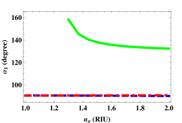
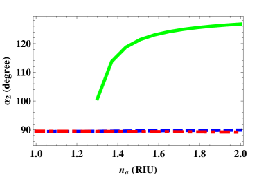
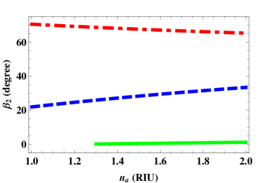
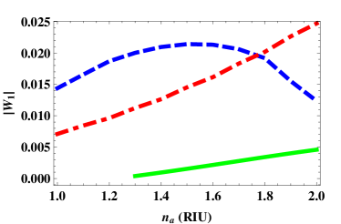
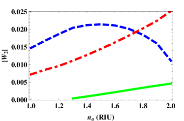
Figure 1: The Euler angles $\alpha_{1,2}$, $\beta_{1,2}$, and the absolute value of the quantities $W_{1,2}$, plotted versus refractive index $n_{a}$ for anisotropy parameter values $\tau=10$ (blue, dashed curves), $1$ (green, solid curves), and $0.1$ (red, broken dashed curves). Values for the other component material parameters are provided in the main text. The quantities $|W_{1,2}|$ plotted for $\tau=1$ are scaled by 100.

The Euler angles $\alpha_{1,2}$ and $\beta_{1,2}$, together with the corresponding values of $|W_{1,2}|$, are plotted versus $n_{a}\in\left(1,2\right)$ in Fig. 1 for three different values of the anisotropy parameter: $\tau=10$ (blue, dashed curves), $1$ (green, solid curves), and $0.1$ (red, broken dashed curves). In the case of $\tau=1$, the quantity $W$ becomes zero-valued for $n_{a}<1.3$; accordingly $\tau=1$ graphs are provided only for $n_{a}\in\left(1.3,2.0\right)$. For the calculations of Fig. 1, the volume fraction $f_{a}=0.25$, the eccentricity parameter $\rho=0.01$, the orientation angle $\varphi=60^{\circ}$, the dissipation parameter $\delta=0.1$, and the dimensionless size parameter $k_{\scriptscriptstyle 0}\eta=0.2$.

For $\tau=1$, the plots of $\alpha_{1}$ and $\alpha_{2}$ both vary rapidly as $n_{a}$ increases from 1.3, whereas the plots of $\beta_{1}$ and $\beta_{2}$ remain almost constant. The corresponding plots of $|W_{1,2}|$ vary little but most importantly these quantities are non-zero for this range of $n_{a}$. For $\tau=10$, the plots of $\beta_{1}$ and $\beta_{2}$ both increase markedly as $n_{a}$ increases, whereas the plots of $\alpha_{1}$ and $\alpha_{2}$ remain almost constant. Furthermore, the plots of $\beta_{1}$ and $\beta_{2}$ are almost the same (but not exactly the same). The corresponding values of $|W_{1,2}|$ are non-zero. For $\tau=0.1$ the plots of $\alpha_{1,2}$ and $\beta_{1,2}$ are qualitatively similar to those for the $\tau=10$ case, except that the plots of $\beta_{1,2}$ versus $n_{a}$ have negative gradients.

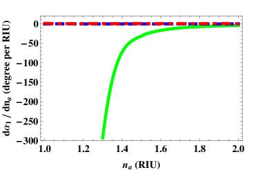
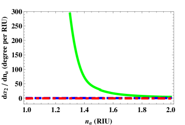
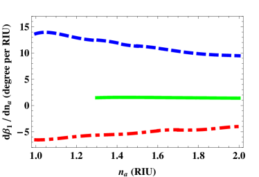
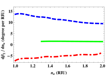
Figure 2: As Fig. 1 but with the derivatives $d\alpha_{1,2}/dn_{a}$ and $d\beta_{1,2}/dn_{a}$ plotted versus refractive index $n_{a}$.

From the point of view of possible optical sensing applications, the sensitivity of the directions which support VWP to small changes in $n_{a}$ is important. Measures of these sensitivities are provided by the derivatives $d\alpha_{1,2}/dn_{a}$ and $d\beta_{1,2}/dn_{a}$. In Fig. 2 plots of $d\alpha_{1,2}/dn_{a}$ and $d\beta_{1,2}/dn_{a}$ versus refractive index $n_{a}$ are presented. For $\tau=1$, the greatest sensitivities arise for $n_{a}$ values close to 1.3, where the maximum values of $|d\alpha_{1,2}/dn_{a}|$ are approximately $300^{\circ}$ per RIU. For $\tau=10$ and $0.1$, the greatest sensitivities arise for $n_{a}$ values close to 1.0, where the maximum values of $|d\beta_{1,2}/dn_{a}|$ are approximately $14^{\circ}$ per RIU and $6.5^{\circ}$ per RIU , respectively.

In order to focus on parameter regimes which yield the greatest sensitivities, henceforth the anisotropy parameter is held constant at $\tau=1$. Also, the quantities $|W_{1,2}|$ have little significance apart from being non-zero; accordingly plots of these quantities are not presented henceforth.

4.3.2 Volume fraction

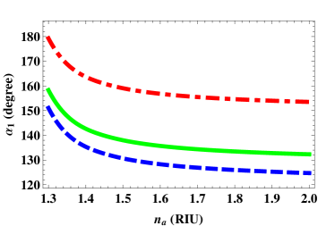
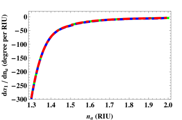
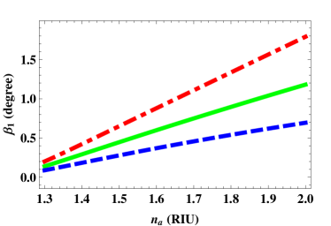
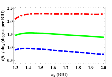
Figure 3: The Euler angles $\alpha_{1}$ and $\beta_{1}$, and the derivatives $d\alpha_{1}/dn_{a}$ and $d\beta_{1}/dn_{a}$, plotted versus refractive index $n_{a}$ for volume fractions $f_{a}=0.1$ (blue, dashed curves), $0.25$ (green, solid curves), and $0.5$ (red, broken dashed curves). Values for the other component material parameters are provided in the main text.

The Euler angles $\alpha_{1}$ and $\beta_{1}$, and the derivatives $d\alpha_{1}/dn_{a}$ and $d\beta_{1}/dn_{a}$, are plotted versus $n_{a}\in\left(1.3,2\right)$ in Fig. 3 for three different values of the volume fraction: $f_{a}=0.1$ (blue, dashed curves), $0.25$ (green, solid curves), and $0.5$ (red, broken dashed curves). For these calculations the anisotropy parameter $\tau=1$ and the other component material parameters are the same as for Figs. 1 and 2. The angle $\alpha_{1}$ varies markedly as the volume fraction varies; but the degree of sensitivity, as gauged by $d\alpha_{1}/dn_{a}$, is essentially independent of volume fraction. In contrast, the angle $\beta_{1}$ is much less dependent upon volume fraction; the sensitivity measure $|d\beta_{1}/dn_{a}|$ is greater for larger volume fractions but the maximum value of this quantity is much smaller than the maximum value of the sensitivity measure $|d\alpha_{1}/dn_{a}|$.

The corresponding plots for $\alpha_{2}$ (not shown) are qualitatively similar to those for $\alpha_{1}$ except that signs of the gradients of the graphs are reversed. The corresponding plots for $\beta_{2}$ (not shown) are almost identical to those for $\beta_{1}$. In fact, as these characteristics apply to all our numerical calculations, henceforth we will only present the results for $\alpha_{1}$ and $\beta_{1}$.

4.3.3 Eccentricity parameter

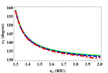
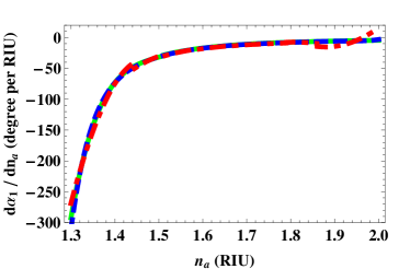
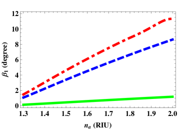
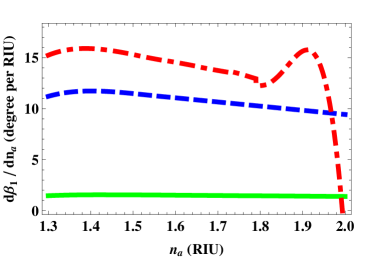
Figure 4: The Euler angles $\alpha_{1}$ and $\beta_{1}$, and the derivatives $d\alpha_{1}/dn_{a}$ and $d\beta_{1}/dn_{a}$, plotted versus refractive index $n_{a}$ for eccentricity parameter values $\rho=0.01$ (green, solid curves), $1$ (blue, dashed curves), and $9$ (red, broken dashed curves). Values for the other component material parameters are provided in the main text.

The Euler angles $\alpha_{1}$ and $\beta_{1}$, and the derivatives $d\alpha_{1}/dn_{a}$ and $d\beta_{1}/dn_{a}$, are plotted versus $n_{a}\in\left(1.3,2\right)$ in Fig. 4 for three different values of the eccentricity parameter: $\rho=0.01$ (green, solid curves), $1$ (blue, dashed curves), and $9$ (red, broken dashed curves). For these calculations the anisotropy parameter $\tau=1$ and the other component material parameters are the same as for Figs. 1 and 2. The angle $\alpha_{1}$ is largely independent of the eccentricity parameter, and likewise the sensitivity measure $d\alpha_{1}/dn_{a}$ is also largely independent of the eccentricity parameter. In contrast, the angle $\beta_{1}$ does vary considerably as $\rho$ varies; the sensitivity measure $|d\beta_{1}/dn_{a}|$ is generally larger for more eccentric particle shapes however the maximum value of this quantity is much smaller than the maximum value of the sensitivity measure $|d\alpha_{1}/dn_{a}|$.

4.3.4 Particle orientation angle

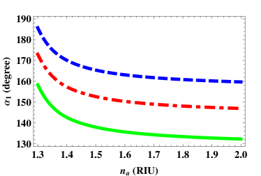
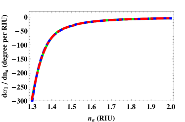
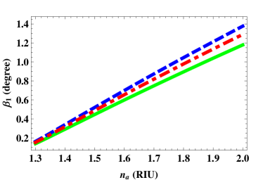
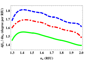
Figure 5: The Euler angles $\alpha_{1}$ and $\beta_{1}$, and the derivatives $d\alpha_{1}/dn_{a}$ and $d\beta_{1}/dn_{a}$, plotted versus refractive index $n_{a}$ for particle orientation angles $\varphi=30^{\circ}$ (blue, dashed curves), $45^{\circ}$ (red, broken dashed curves), and $60^{\circ}$ (green, solid curves). Values for the other component material parameters are provided in the main text.

The Euler angles $\alpha_{1}$ and $\beta_{1}$, and the derivatives $d\alpha_{1}/dn_{a}$ and $d\beta_{1}/dn_{a}$, are plotted versus $n_{a}\in\left(1.3,2\right)$ in Fig. 5 for three different values of the particle orientation angle: $\varphi=30^{\circ}$ (blue, dashed curves), $45^{\circ}$ (red, broken dashed curves), and $60^{\circ}$ (green, solid curves). For these calculations the anisotropy parameter $\tau=1$ and the other component material parameters are the same as for Figs. 1 and 2. The angle $\alpha_{1}$ varies considerably as $\varphi$ varies but the sensitivity measure $d\alpha_{1}/dn_{a}$ is largely independent of $\varphi$. On the other hand, the angle $\beta_{1}$ varies very little as $\varphi$ varies; the sensitivity measure $|d\beta_{1}/dn_{a}|$ is slightly larger at smaller values of $\varphi$ but the maximum value of this quantity is much smaller than the maximum value of the sensitivity measure $|d\alpha_{1}/dn_{a}|$.

4.3.5 Dissipation parameter

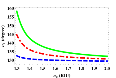
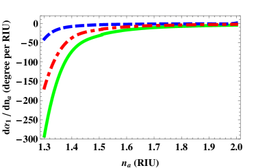
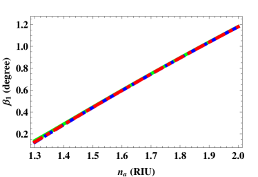
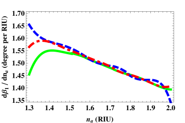
Figure 6: The Euler angles $\alpha_{1}$ and $\beta_{1}$, and the derivatives $d\alpha_{1}/dn_{a}$ and $d\beta_{1}/dn_{a}$, plotted versus refractive index $n_{a}$ for dissipation parameter values $\delta=0.01$ (blue, dashed curves), $0.05$ (red, broken dashed curves), and $0.1$ (green, solid curves). Values for the other component material parameters are provided in the main text.

The Euler angles $\alpha_{1}$ and $\beta_{1}$, and the derivatives $d\alpha_{1}/dn_{a}$ and $d\beta_{1}/dn_{a}$, are plotted versus $n_{a}\in\left(1.3,2\right)$ in Fig. 6 for three different values of the dissipation parameter: $\delta=0.01$ (blue, dashed curves), $0.05$ (red, broken dashed curves), and $0.1$ (green, solid curves). For these calculations the anisotropy parameter $\tau=1$ and the other component material parameters are the same as for Figs. 1 and 2. The angle $\alpha_{1}$ varies markedly as $\delta$ varies; the sensitivity measure $d\alpha_{1}/dn_{a}$ also varies considerably as $\delta$ varies, especially so at small values of $n_{a}$. We note that larger values of $|d\alpha_{1}/dn_{a}|$ are attained at larger values of $\delta$. On the other hand, the angle $\beta_{1}$ is essentially independent of the dissipation parameter; very small changes in the sensitivity measure $d\beta_{1}/dn_{a}$ are observed as $\delta$ varies, most conspicuously at smaller values of $n_{a}$. As in Figs. 2–5, the largest values of the sensitivity measure $|d\beta_{1}/dn_{a}|$ are much smaller than the largest values of the sensitivity measure $|d\alpha_{1}/dn_{a}|$.

4.3.6 Size parameter

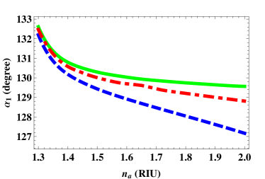
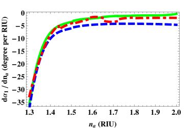
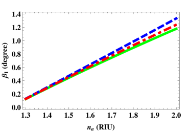
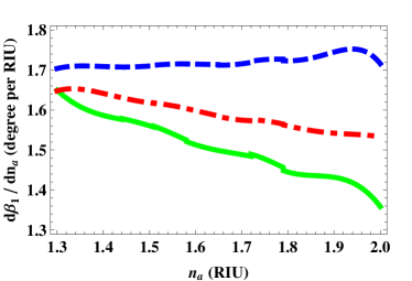
Figure 7: The Euler angles $\alpha_{1}$ and $\beta_{1}$, and the derivatives $d\alpha_{1}/dn_{a}$ and $d\beta_{1}/dn_{a}$, plotted versus refractive index $n_{a}$ for dimensionless size parameter values $k_{\scriptscriptstyle 0}\eta=0.2$ (green, solid curves), $0.3$ (red, broken dashed curves), and $0.4$ (blue, dashed curves). Values for the other component material parameters are provided in the main text.

The Euler angles $\alpha_{1}$ and $\beta_{1}$, and the derivatives $d\alpha_{1}/dn_{a}$ and $d\beta_{1}/dn_{a}$, are plotted versus $n_{a}\in\left(1.3,2\right)$ in Fig. 7 for three different values of the dimensionless size parameter: $k_{\scriptscriptstyle 0}\eta=0.2$ (green, solid curves), $0.3$ (red, broken dashed curves), and $0.4$ (blue, dashed curves). For these calculations the anisotropy parameter $\tau=1$, the dissipation parameter $\delta=0.01$, and the other component material parameters are the same as for Figs. 1 and 2. The angle $\alpha_{1}$ varies moderately as $\varphi$ varies, most obviously at larger values of $n_{a}$; the sensitivity measure $d\alpha_{1}/dn_{a}$ varies only slightly as $k_{\scriptscriptstyle 0}\eta$ varies, most obviously at larger values of $n_{a}$. Slightly larger values of $|d\alpha_{1}/dn_{a}|$ are attained at smaller values of $k_{\scriptscriptstyle 0}\eta$. In a similar vein, both the angle $\beta_{1}$ and $d\beta_{1}/dn_{a}$ vary moderately as $k_{\scriptscriptstyle 0}\eta$ varies, most obviously at larger values of $n_{a}$. The largest values of $d\beta_{1}/dn_{a}$ are attained at larger values of $n_{a}$ for larger values of $k_{\scriptscriptstyle 0}\eta$. However, as in Figs. 2–6, the largest values of the sensitivity measure $|d\beta_{1}/dn_{a}|$ are much smaller than the largest values of the sensitivity measure $|d\alpha_{1}/dn_{a}|$.

5 Closing remarks

For a porous biaxial dielectric host material infiltrated by a material of refractive index $n_{a}$, our numerical studies have revealed sensitivities of up to $300^{\circ}$ per RIU for the directions which support VWP. The sensitivities achieved are acutely dependent upon the degrees of anisotropy and dissipation of the host material, and the refractive index $n_{a}$. The orientations, shapes and sizes of the particles which constitute the component materials exert only a secondary influence on the maximum sensitivities achieved. Also, for the parameter ranges considered, the volume fraction has little effect on the maximum sensitivities achieved.

These numerical findings bode well for the possible harnessing of VWP for optical sensing applications. Such sensitivities of up to $300^{\circ}$ per RIU compare favourably to sensitivities reported for optical sensing based on the excitation of surface-plasmon-polariton waves [19, 20, 21]. In particular, the maximum sensitivities reported in recent studies involving surface-plasmon-polariton waves excited at the planar surfaces of sculptured thin films are an order of magnitude smaller than those found here for VWP [22, 23, 24].

In the parameter regimes where the greatest sensitivities for VWP were found , only one of the Euler angles ($\alpha$ in Figs. 2–7) varied sharply whereas the other Euler angle ($\beta$ in Figs. 2–7) remained almost constant as $n_{a}$ varied. Thus, if one were to track the directions of VWP in such parameter regimes then the tracking may only need to be done in one plane. This may prove to be a helpful feature in the possible harnessing of VWP for optical sensing applications. Further studies are needed to identify practical configurations for the harnessing of VWP for optical sesning applications.

Appendix 1: The extended Bruggeman formalism

The extended Bruggeman formalism is based on the nonlinear dyadic equation [25, 26]

$$f_{a}\left\{\left(\underline{\underline{\epsilon}}_{\,a}-\underline{\underline{\epsilon}}_{\,HCM}\right)\cdot\left[\underline{\underline{I}}+\underline{\underline{D}}_{\,a}\cdot\left(\underline{\underline{\epsilon}}_{\,a}-\underline{\underline{\epsilon}}_{\,HCM}\right)\right]^{-1}\right\}+f_{b}\left\{\left(\underline{\underline{\epsilon}}_{\,b}-\underline{\underline{\epsilon}}_{\,HCM}\right)\cdot\left[\underline{\underline{I}}+\underline{\underline{D}}_{\,b}\cdot\left(\underline{\underline{\epsilon}}_{\,b}-\underline{\underline{\epsilon}}_{\,HCM}\right)\right]^{-1}\right\}=\underline{\underline{0}}\,.$$ (13)

Under the extended formalism, the depolarization dyadics $\underline{\underline{D}}_{\,a,b}$ are viewed as the sums [27]

$$\underline{\underline{D}}_{\,\ell}=\underline{\underline{D}}^{0}_{\,\ell}+\underline{\underline{D}}^{+}_{\,\ell},\qquad(\ell=a,b),$$ (14)

wherein the term $\underline{\underline{D}}^{0}_{\,\ell}$ represents the depolarization contribution arising from a vanishingly small ellipsoidal particle of shape specified by the surface dyadic $\underline{\underline{U}}_{\,\ell}$. We have the double integral formula [28, 29]

$$\underline{\underline{D}}^{0}_{\,\ell}=\frac{1}{4\pi}\,\int^{2\pi}_{\phi=0}\int^{\pi}_{\theta=0}\frac{\left(\underline{\underline{U}}^{-1}_{\,\ell}\cdot\hat{{\bf q}}\right)\,\left(\underline{\underline{U}}^{-1}_{\,\ell}\cdot\hat{{\bf q}}\right)\;\sin\theta}{\left(\underline{\underline{U}}^{-1}_{\,\ell}\cdot\hat{{\bf q}}\right)\cdot\underline{\underline{\epsilon}}_{\,HCM}\cdot\left(\underline{\underline{U}}^{-1}_{\,\ell}\cdot\hat{{\bf q}}\right)}\,d\theta\,d\phi\,,\qquad(\ell=a,b),$$ (15)

with the unit vector $\hat{{\bf q}}=\sin\theta\cos\phi\,\hat{{\bf x}}+\sin\theta\sin\phi\,\hat{{\bf y}}+\cos\theta\,\hat{{\bf z}}$. The contribution to the depolarization dyadic arising specifically from the nonzero size of the component particles is represented by the dyadic term $\underline{\underline{D}}^{+}_{\,\ell}$. It is convenient to express this dyadic as a subdyadic of the 6$\times$6 dyadic $\underline{\underline{\mathbb{D}}}^{+}_{\,\ell}$, as defined via

$$\left[\,\underline{\underline{D}}^{+}_{\,\ell}\,\right]_{mn}=\left[\,\underline{\underline{\mathbb{D}}}^{+}_{\,\ell}\,\right]_{mn},\qquad\left(m,n\in\left\{1,2,3\right\}\right).$$ (16)

Here [27]

$$\underline{\underline{\mathbb{D}}}^{+}_{\,\ell} = \frac{\omega^{4}}{4\pi\mu_{\scriptscriptstyle 0}}\int^{2\pi}_{\phi=0}\int^{\pi}_{\theta=0}\frac{\sin\theta}{\left[\left(\underline{\underline{U}}^{-1}_{\,\ell}\cdot\hat{{\bf q}}\right)\cdot\underline{\underline{\epsilon}}_{\,HCM}\cdot\left(\underline{\underline{U}}^{-1}_{\,\ell}\cdot\hat{{\bf q}}\right)\right]\left(\underline{\underline{U}}^{-1}_{\,\ell}\cdot\hat{{\bf q}}\right)\cdot\left(\underline{\underline{U}}^{-1}_{\,\ell}\cdot\hat{{\bf q}}\right)}$$

$$\times\Bigg{[}\frac{1}{\kappa_{+}-\kappa_{-}}\Bigg{(}\frac{\exp\left(i\eta q\right)}{2q^{2}}\left(1-i\eta q\right)\Big{\{}\,\mbox{det}\left[\underline{\underline{\mathbb{A}}}(\underline{\underline{U}}^{-1}_{\,\ell}\cdot{\bf q})\right]\,\underline{\underline{\mathbb{G}}}^{+}(\underline{\underline{U}}^{-1}_{\,\ell}\cdot{\bf q})$$

$$+\mbox{det}\left[\underline{\underline{\mathbb{A}}}(-\underline{\underline{U}}^{-1}_{\,\ell}\cdot{\bf q})\right]\,\underline{\underline{\mathbb{G}}}^{+}(-\underline{\underline{U}}^{-1}\cdot{\bf q})\Big{\}}\Bigg{)}^{q=\sqrt{\kappa_{+}}}_{q=\sqrt{\kappa_{-}}}+\frac{\mbox{det}\left[\underline{\underline{\mathbb{A}}}({\bf 0})\right]}{\kappa_{+}\,\kappa_{-}}\,\underline{\underline{\mathbb{G}}}^{+}({\bf 0})\Bigg{]}\;d\theta\;d\phi,\qquad(\ell=a,b),$$

wherein $\kappa_{\pm}$ are the $q^{2}$ roots of $\mbox{det}\left[\underline{\underline{\mathbb{A}}}(\underline{\underline{U}}^{-1}\cdot{\bf q})\right]=0$, the vector ${\bf q}=q\,\hat{{\bf q}}$, and the 6$\times$6 dyadics

$$\underline{\underline{\mathbb{A}}}({\bf p})=\left[\begin{array}[]{cc}\underline{\underline{\epsilon}}_{\,HCM}&\left({\bf p}/\omega\right)\times\underline{\underline{I}}\vspace{2mm}\\ -\left({\bf p}/\omega\right)\times\underline{\underline{I}}&\mu_{\scriptscriptstyle 0}\,\underline{\underline{I}}\end{array}\right]$$ (18)

and

$$\underline{\underline{\mathbb{G}}}^{+}({\bf p})=\underline{\underline{\mathbb{A}}}^{-1}({\bf p})-\lim_{|{\bf p}|\to\infty}\underline{\underline{\mathbb{A}}}^{-1}({\bf p}).$$ (19)

The HCM permittivity dyadic $\underline{\underline{\epsilon}}_{\,HCM}$ may be extracted from the nonlinear dyadic equation (13) by standard numerical techniques, such as the Jacobi technique [30].

Appendix 2: Estimates of the HCM’s constitutive parameters

Here estimates of the extended Bruggeman estimates of the HCM’s relative permittivity parameters $\epsilon_{x,y,z,t}$ are presented. Component material $a$ is specified by $n_{a}=1.5$ while component material $b$ is specified by the anisotropy parameter $\tau=1$ and dissipation parameter $\delta=0.1$, per Eqns. (12). In Fig. 8, the real and imaginary parts of $\epsilon_{x,y,z,t}$ are plotted as functions of particle orientation angle $\varphi$ and volume fraction $f_{a}$; for these calculations the dimensionless size parameter $k_{\scriptscriptstyle 0}\eta=0.2$ and the particle eccentricity parameter $\rho=9$. In Fig. 9, the real and imaginary parts of $\epsilon_{x,y,z,t}$ are plotted against dimensionless size parameter $k_{\scriptscriptstyle 0}\eta$ and the particle eccentricity parameter $\rho$; for these calculations the volume fraction $f_{a}=0.25$ and the particle orientation angle $\varphi=45^{\circ}$. For comprehensive discussions on the relationships between the extended (and non-extended) Bruggeman estimates of the HCM’s relative permittivity parameters and the parameters which characterize the component materials, the reader is referred to earlier works [10, 11, 12].

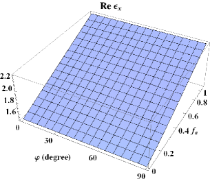
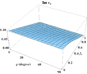
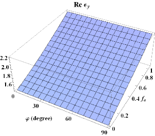
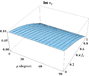
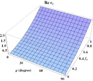
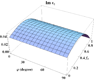
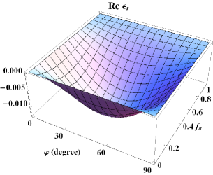
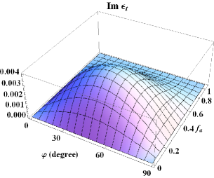
Figure 8: Real and imaginary parts of the extended Bruggeman estimates of relative permittivity parameters of the HCM plotted versus volume fraction $f_{a}\in\left(0,1\right)$ and particle orientation angle $\varphi\in\left(0^{\circ},90^{\circ}\right)$. The dimensionless size parameter $k_{\scriptscriptstyle 0}\eta=0.2$, the dissipation parameter $\delta=0.1$, the anisotropy parameter $\tau=1$, and the particle eccentricity parameter $\rho=9$.

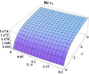
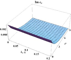
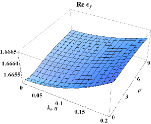
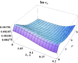
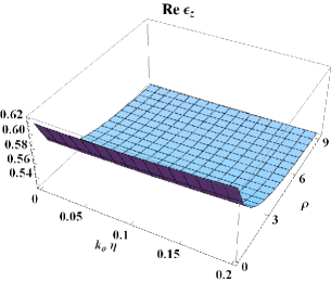
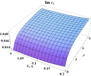
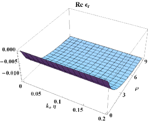
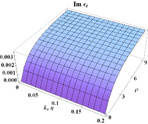
Figure 9: As Fig. 8 except that the HCM’s relative permittivity parameters are plotted versus the dimensionless size parameter $k_{\scriptscriptstyle 0}\eta\in\left(0,0.2\right)$ and the particle eccentricity parameter $\rho\in\left(0,9\right)$. The volume fraction $f_{a}=0.25$ and particle orientation angle $\varphi=45^{\circ}$.

References

- [1] M. Born and E. Wolf, Principles of Optics, 6th Edition, Pergamon Press, Oxford, UK (1980).
- [2] A. P. Khapalyuk, “On the theory of circular optical axes,” Opt. Spectrosc. (USSR) 12, 52–54 (1962).
- [3] W. Voigt, “On the behaviour of pleochroitic crystals along directions in the neighbourhood of an optic axis,” Phil. Mag. 4, 90–97 (1902).
- [4] S. Pancharatnam, “The optical interference figures of amethystine quartz — Part II,” Proc. Ind. Acad. Sci. A 47, 210–229 (1958).
- [5] F. I. Fedorov and A. M. Goncharenko, “Propagation of light along the circular optical axes of absorbing crystals,” Opt. Spectrosc. (USSR) 14, 51–53 (1963).
- [6] V. M. Agranovich and V. L. Ginzburg, Crystal Optics with Spatial Dispersion, and Excitons, Springer, Berlin, Germany (1984).
- [7] B. N. Grechushnikov and A. F. Konstantinova, “Crystal optics of absorbing and gyrotropic media,” Comput. Math. Applic. 16, 637–655 (1988).
- [8] A. Lakhtakia, “Anomalous axial propagation in helicoidal bianisotropic media,” Opt. Commun. 157, 193–201 (1998).
- [9] M. V. Berry, “The optical singularities of bianisotropic crystals,” Proc. R. Soc. Lond. A 461, 2071–2098 (2005).
- [10] T. G. Mackay and A. Lakhtakia, “Voigt wave propagation in biaxial composite materials,” J. Opt. A: Pure Appl. Opt. 5, 91–95 (2003).
- [11] T. G. Mackay and A. Lakhtakia, “Correlation length facilitates Voigt wave propagation,” Waves Random Media 14, L1–L11 (2004).
- [12] T. G. Mackay, “Voigt waves in homogenized particulate composites based on isotropic dielectric components,” J. Opt. 13, 105702 (2011).
- [13] T. G. Mackay, “On extended homogenization formalisms for nanocomposites,” J. Nanophotonics 2, 021850 (2008).
- [14] T. G. Mackay and A. Lakhtakia, “Electromagnetic fields in linear bianisotropic mediums,” Prog. Opt. 51, 121–209 (2008).
- [15] T. G. Mackay and W. S. Weiglhofer, “Homogenization of biaxial composite materials: Nondissipative dielectric properties,” Electromagnetics 21, 15–25 (2001).
- [16] T. G. Mackay and W. S. Weiglhofer, “Homogenization of biaxial composite materials: dissipative anisotropic properties,” J. Opt. A: Pure Appl. Opt. 2, 426–432 (2000).
- [17] G. B. Arfken and H. J. Weber, Mathematical Methods for Physicists, 4th Edition, Academic Press, London, UK (1995).
- [18] J. Gerardin and A. Lakhtakia, “Conditions for Voigt wave propagation in linear, homogeneous, dielectric mediums,” Optik 112, 493–495 (2001).
- [19] J. Homola (Ed.), Surface Plasmon Resonance Based Sensors, Springer, Heidelberg, Germany (2006).
- [20] I. Abdulhalim, M. Zourob, and A. Lakhtakia, Surface plasmon resonance for biosensing: A mini-review, Electromagnetics 28, 214–242 (2008).
- [21] A. Shalabney and I. Abdulhalim, “Sensitivity enhancement methods for surface plasmon sensors,” Lasers Photon. Rev.,” 5, 571–606 (2011).
- [22] J. A. Polo, Jr., T. G. Mackay and A. Lakhtakia, “Mapping multiple surface-plasmon-polariton-wave modes at the interface of a metal and a chiral sculptured thin film,” J. Opt. Soc. Amer. B 28, 2656–2666 (2011).
- [23] T. G. Mackay and A. Lakhtakia, “Modeling chiral sculptured thin films as platforms for surface–plasmonic–polaritonic optical sensing,” IEEE Sensors J. 12, 273–280 (2012).
- [24] S. S. Jamaian and T. G. Mackay, “On columnar thin films as platforms for surface-plasmonic-polaritonic optical sensing: higher-order considerations,” Opt. Commun. 285, 5535–5542 (2012).
- [25] W. S. Weiglhofer, A. Lakhtakia and B. Michel, “Maxwell Garnett and Bruggeman formalisms for a particulate composite with bianisotropic host medium,” Microwave Opt. Technol. Lett. 15, 263–266 (1997); Erratum: 22, 221 (1999).
- [26] T. G. Mackay, “Effective constitutive parameters of linear nanocomposites in the long-wavelength regime,” J. Nanophotonics 5, 051001 (2011).
- [27] T. G. Mackay, “Depolarization volume and correlation length in the homogenization of anisotropic dielectric composites,” Waves Random Media 14, 485–498 (2004); Erratum: Waves Random Complex Media 16, 85 (2006).
- [28] B. Michel, “A Fourier space approach to the pointwise singularity of an anisotropic dielectric medium,” Int. J. Appl. Electromagn. Mech. 8, 219–227 (1997).
- [29] B. Michel and W. S. Weiglhofer, “Pointwise singularity of dyadic Green function in a general bianisotropic medium,” Arch. Elekron. Übertrag. 51, 219–223 (1997); Erratum: 52, 31 (1998).
- [30] B. Michel, A. Lakhtakia and W.S. Weiglhofer, Homogenization of linear bianisotropic particulate composite media — Numerical studies, Int. J. Appl. Electromag. Mech. 9 (1998), 167–178; Erratum: 10 (1999), 537–538.